The density of states approach for the simulation of finite density quantum field theories

Abstract

Finite density quantum field theories have evaded first principle Monte-Carlo simulations due to the notorious sign-problem. The partition function of such theories appears as the Fourier transform of the generalised density-of-states, which is the probability distribution of the imaginary part of the action. With the advent of Wang-Landau type simulation techniques and recent advances [1], the density-of-states can be calculated over many hundreds of orders of magnitude. Current research addresses the question whether the achieved precision is high enough to reliably extract the finite density partition function, which is exponentially suppressed with the volume. In my talk, I review the state-of-play for the high precision calculations of the density-of-states as well as the recent progress for obtaining reliable results from highly oscillating integrals. I will review recent progress for the $Z_{3}$ quantum field theory for which results can be obtained from the simulation of the dual theory, which appears to free of a sign problem.

1 Introduction

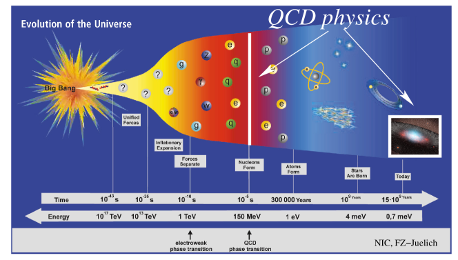
Figure 1: QCD impact on the evolution of the early Universe.

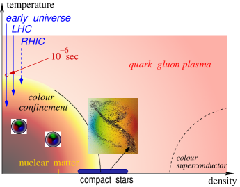
Figure 2: Sketch of the QCD phase diagram.

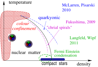
Figure 3: QCD phase diagram: first principle calculations and model building.

The properties of strongly interacting matter has sparked many important investigations using accelerator experiments and large scale theoretical studies. In an astrophysical context, the theory of interactions, QCD, dominates the area around $10^{-6}$ seconds after the Big Bang when quark matter confines to colour neutral hadrons. Since QCD captures the impact of the strong nuclear forces, it is widely believed that QCD plays an essential role to understand compact star matter as it may exist nowadays e.g. in neutron stars (see figure 1 for an illustration). The so-called QCD phase diagram characterises the states of matter as a function of the density and temperature in a 2d graph. Completing this diagram in its extreme regions and in particular for cold and dense matter is an outstanding problem which still triggers model building and new techniques for computer simulation after 30 years of intense research. Under moderate conditions, quarks and gluons are confined to colour-neutral hadrons, while this confinement feature of QCD is believed to cease to exist under extreme conditions, temperatures and/or densities. In the early universe before the QCD phase transition roughly at time $10^{-6}$ seconds, matter has not yet clustered due to gravity and, as a result, the density is very low compared to e.g. nuclear matter density. Similarly, the conditions in heavy ion collision experiments carried out at RHIC (located at Brookhaven National Laboratory (BNL) in Upton, New York) or LHC (built by the European Organization for Nuclear Research (CERN)) produce very hot matter at low densities. From an experimental point of view, very little is known even at moderate densities let alone the cold and dense regime of compact star matters (see figure 3).

Lattice gauge simulations offer first principle non-perturbative results with good control over the errors. Markov chain Monte-Carlo simulations can be very successfully applied and reliable results for the states of matter can be obtained at all temperatures and small baryon chemical potentials (shaded area in figure 3, see e.g. [2] for a review). Over the recent years, many new models have been developed to describe QCD matter at high densities: quarkyonic matter is motivated by the so-called ’t Hooft limit of the hypothetical theory with a large number of colours and sees the quarks deconfined inside the Fermi sphere while only the baryons at the surface of the Fermi sphere undergo colour confinement—[3]. The chiral magnetic effect [4] takes into account the strong magnetic field that are produced by the colliding charges in heavy ion experiments and uses an effective quark model to estimate their impact on the QCD phase structure. In the confinement phase, quarks in a certain gluonic background can change their statistics from Fermi to Bose type. At moderate densities, these so-called centre dressed and confined quarks therefore might undergo Bose condensation leading to to new state of cold and confined matter [5]. None of these ideas have yet been tested by first principle calculations. At a finite baryon chemical potential, the QCD action acquires an imaginary part, and, hence, standard Monte-Carlo techniques cannot be applied for the lattice simulation of QCD at finite densities. This has become known as the notorious sign problem. Early attempts pursued Monte-Carlo simulations with the modulus of the quark determinant and included the phase factor to the observable to be calculated. It turns out that the expectation value of the phase factor is very small (see [6] for an illustration) showing that the such generated Monte-Carlo configurations contain very little information on finite density QCD. The sign problem has turned into an overlap problem.

The recent past has seen a renaissance of ideas targeting dense and cold fermionic matter. Some of the methods were proposed some time ago, but have now reached an unprecedented level of sophistication. The reweighting approach proposed by Fodor and Katz [7] uses a multi-parameter action to optimise the overlap. This method is particularly suited for intermediate temperatures and might possess a reach that covers the critical endpoint of the QCD phase diagram [8]. Langevin simulations of lattice gauge theories avoid the positivity constraint of the Gibbs factor, which lies at the heart of Monte-Carlo simulations, and might therefore be suitable for finite density simulations [9, 10]. This technique regained a lot of interest when Aarts showed that stochastic quantisation can evade the sign problem at least for the relativistic Bose gas [11, 12]. Although the conceptional question whether the approach converges to the correct answer [13] is still under active investigations, the approach is one of the few methods that are currently applied to finite density QCD [14]. It might appear that integrating the gluonic degrees of freedom before the fermion fields alleviates the sign problem. This could be done e.g. in the strong coupling limit [15] leading to a description of Nuclear Physics suiting lattice simulations [16]. It was observed in 1d QCD that even integrating part of the gluonic degrees of freedom leads to substantial improvements [17]. Finally, a reformulation of the theory might improve on the sign the problem or remove it altogether. Indeed, theories the dual of which are real are then accessible by standard Monte-Carlo techniques. Example for complex action spin models that are real upon dualisation are $Z_{3}$ spin model [18] or the $O(2)$ model at finite densities [19, 20]. These models can be efficiently simulated using worm type algorithms [21]. Alternative lattice discretisations [22] and spin blocking techniques in combination with the (tensor) renormalisation group approach [23] might be equally successful to eliminate the sign problem from Yang-Mills theories. Also not hinging on a real dualisation of the theory is the fermion bag approach approach by Chandrasekharan [24] for which the sign problem is relegated to finite size fermion bags. This approach has been seen to be very efficient for fermion theories with four-fermion coupling such as the Thirring model with massless fermions on large lattices [25].

An efficient alternative to conventional Monte-Carlo simulations is based upon the numerical computation of the density of states using the multi-canonical algorithm [27] or a Wang-Landau type strategy [26]. A modified version of the Wang-Landau method is the LLR algorithm [1], which is effective for theories with continuous degrees of freedom as opposed to spin models (see also [28]). The latter algorithm has been extended from the calculation of the action distribution to accessing probability distributions of other extensive quantities such as the SU(2) Polyakov line [29]. Furthermore, it has been proposed in [30] to use LLR techniques for a high precision calculation of the distribution of the imaginary part of the action. Once this quantity has been determined, the partition function of the complex theory can be computed semi-analytically by carrying out the Fourier transform of the corresponding probability distribution [30]. Below, we will summarise the state of affairs concerning density-of-states methods and the LLR algorithm in particular to simulate theories with a sign problem. An overview on selected new methods solving the sign problem can be found in the recent review by Aarts [31].

2 Density-of-states approach to complex action systems

2.1 Density-of-states and the overlap problem

Let us consider the partition function $Z$ of a theory of one degree of freedom $\phi$ with a complex action:

$$Z=\int{\cal D}\phi\;\exp\{\beta S_{R}[\phi]+i\mu S_{I}[\phi]\}$$ (1)

where $\mu$ is the “chemical potential”, and $S_{R/I}$ are real and imaginary parts of the action. We introduce the generalised density of states [30] by

$$P_{\beta}(s)=\int{\cal D}\phi\;\delta\Bigl{(}s-S_{I}[\phi]\Bigr{)}\;\exp\{\beta S_{R}[\phi]\}\;.$$ (2)

For $\beta=0$, $P_{0}(s)$ just counts the number of states with the constraint that the imaginary part of the action is given by $s$. At finite $\beta$, the number count is weighted by the “Gibbs” factor $\exp\{\beta S_{R}[\phi]\}$. Once $P_{\beta}(s)$ is known, the task to calculate the partition function boils down to evaluate the integral

$$Z(\beta,\mu)\;=\;\int ds\;P_{\beta}(s)\;\exp\{i\,\mu\,s\}.$$ (3)

Since the integrand in (2) is perfectly real, the difficulties with the sign problem are relegated to the 1-dimensional integral (3). In fact, $P_{\beta}(s)$ could be estimated by performing a standard Monte-Carlo simulation with the Gibbs factor $\exp\{\beta S_{R}[\phi]\}$ and to bin the values for $S_{I}$ in a histogram. The LLR algorithm will provide us with $\beta=0$, $P_{0}(s)$ over hundreds of orders of magnitude (see below for an example). The aim of this paper is to discuss the options for a calculation of the highly oscillating integral (3).

Let us scope the amount of difficulty that resides with this task. We firstly note that the action $S_{i}$ is an extensive quantity $S_{I}(\phi)=Vs_{I}$ with $V$ the number of degrees of freedom (volume) and with the action density $s_{i}$ of order one. A good qualitative choice (see e.g. [20]) is given by

$$P_{\beta}(s)=\exp\Bigl{\{}-\frac{s^{2}}{V}\Bigr{\}}\hbox to28.45274pt{\hfill}\hbox{leading to }\hbox to28.45274pt{\hfill}Z\;=\;\int ds\;\mathrm{e}^{-s^{2}/{V}}\;\exp\{i\,\mu s\}\;\propto\;{\exp\{-\frac{\mu^{2}}{4}\,{V}\}}\;.$$

For a chemical potential $\mu$ of order one, $Z$ is exponentially suppressed with the number of degrees of freedom $V$. On the other hand, $P_{\beta}(s)$ is only known numerically and of order one at least for small $s$. For a successful evaluation of the integral in $Z$ (3), any numerical method for obtaining $P_{\beta}(s)$ must have the properties

• exponential error suppression for extensive quantities

• for the whole domain of support for $S_{I}$.

The LLR algorithm proposed in [1] just delivers that.

2.2 The $Z_{3}$ spin model as showcase

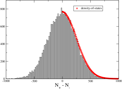
Figure 4: Histogram count for $N_{+}-N_{-}\propto S_{I}$ (linear scale); $24^{3}$ lattice, $\tau=0.17$, $\kappa=0.05$.

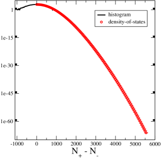
Figure 5: Same histogram on a logarithmic scale with the LLR result now reaching beyond $N_{+}-N_{-}\approx 5,500$.

The key question is whether the quality of the result for $P_{\beta}(s)$ obtained by the LLR algorithm is good enough to admit a reliable calculation of the partition function $Z$ via the integral (3). The answer to this question is model dependent. The 3-dimensional $Z_{3}$ spin model on a cubic lattice at finite density maps onto a real action system upon dualisation and is thus open to standard Monte-Carlo simulations. It serves as a first benchmark test in the feasibility study for our approach to theories with a sign problem. Here, we will review our findings for the 3-dimensional case. Degrees of freedom are the centre elements $z(x)$ that take values from the group $Z_{3}$

$$z(x)\;\in\{1,z_{+},z_{-}\}\;,\hbox to28.45274pt{\hfill}z_{\pm}=(1+i\sqrt{3})/2.$$

The action is given by

$$S[z]={\tau}\sum_{x,\nu}[z_{x}z^{\ast}_{x+\nu}+cc]\;+\;\sum_{x}[{\eta}z_{x}+{\bar{\eta}}z^{\ast}_{x}]\;,\hbox to28.45274pt{\hfill}\eta=\kappa\;\exp(\mu)\;,\;\;\;\bar{\eta}=\kappa\;\exp(-\mu)\;.$$ (4)

This model is inspired by finite density QCD in the heavy quark limit, and the parameter $\tau$ is reminiscent of the temperature and $\kappa$ reflects the quark hopping parameter [18]. Apparently, the action becomes complex as soon as $\mu\not=0$. If for a given configuration $z(x)$ the quantity $N_{\pm}$ represents the number of spins on the lattice with $z=z_{\pm}$, the imaginary part of the action can be written as:

$$S_{I}\;=\;\frac{\eta-\bar{\eta}}{2i}\sum_{x}[z\,-\,z^{\ast}]\;=\;\sqrt{3}\,\kappa\,\mathrm{sinh}(\mu)\;[N_{+}-N_{-}]\;.$$ (5)

We have performed a standard Monte-Carlo simulation using a $24^{3}$ lattice, $\kappa=0.17$ and $\kappa=0.05$ to obtain a histogram for $N_{+}-N_{-}$ (see [30] for details). The result is shown in figure 5 on a linear scale (see figure 5 with the $y$-axis on a logarithmic scale). Note that we have very little “events” with $N_{+}-N_{-}>1000$. For the calculation of the Fourier transform to obtain the partition function $Z$ in (3), the tails with $|N_{+}-N_{-}|\gg 1000$ significantly contribute for $\mu\approx 1$. We recover the overlap problem in the light of the density-of-states approach. Our result for $P(N_{+}-N_{-})$ using the LLR method is also shown in the figures 5 and 5. We find a reassuring agreement with the standard simulation result and moreover we have obtained the distribution $P(N_{+}-N_{-})$ for values as large as $N_{+}-N_{-}=5000$ and over sixty orders of magnitude.

3 The partition function from highly oscillating integrals

3.1 Polynomial fit

Our task is now to carry out the Fourier transform of the generalised density of states $P(s)$ in order to obtain the partition function $Z$ (see (3)). One advantage of our approach is that we can use sophisticated integration techniques, which converge like $1/n^{p}$, $p>1$, where $n$ is the number of evaluations of the integrand. Note that any Monte-Carlo integration that sub-sums the Fourier transform necessarily converges at best like $1/\sqrt{n}$. Note, however, that even the sophisticated integrations techniques would fail for sizeable values of the chemical potential without further knowledge of the function $P(s)$. We have so far studied the density-of-states for the theories $U(1)$, $SU(2)$, $SU(3)$ and $Z_{3}$ and a common feature has been that $log\,P(s)$ is indeed very smooth and, as expected, monotonic functions of its variable $s$. In the present case, we also have the symmetry under reflection $P(s)=P(-s)$. The “smoothness” of $P(s)$ is summarised by the fact that the Taylor expansion

$$\ln\,P(s)\;=\;\sum_{i>0,\mathrm{even}}^{q}c_{i}\,s^{i}\;,\hbox to28.45274pt{\hfill}q=2,4,6,8,\ldots$$ (6)

can produce results that are indistinguishable from the numerical findings for $P(s)$ within error bars. Depending on the region of the parameter space $\beta=(\tau,\kappa)$, $q$ as small as $4$ might be sufficient. As soon as an acceptable representation of the numerical data in terms of the ansatz (6) is found, the calculation of the partition function can be performed in a “semi-analytic” way using advanced numerical integration techniques:

$$Z(\mu)\;=\;2\int ds\;P(s)\;\cos(\mu\,\,s\,)\;=\;2\int ds\;\exp\left\{\sum_{i}^{q}c_{i}s^{i}\right\}\,\cos(\mu\,s)\;.$$ (7)

3.2 Asymptotic referencing

Similar to the scenario in the previous subsection, it might be useful to describe the gross features of $P(s)$ by an analytic function, say $P_{\mathrm{asy}}(s)$ especially for large values $s$. Decomposing

$$P(s)\;=\;\bar{P}(s)\,P_{\mathrm{asy}}(s)\;,$$ (8)

the function $\bar{P}(s)$ might have a moderate range of values although $P(s)$ spans many orders of magnitude. For a technical side-remark, we point out that the LLR algorithm [1] can be easily adapted to directly produce $\bar{P}(s)$ for a given choice for $P_{\mathrm{asy}}(s)$. The partition function is obtained by Fourier transformation:

$$Z(\mu)\;=\;\hbox{FT}[P](\mu)\;=\;\int ds\;P(s)\;\mathrm{e}^{i\mu s}\;=\;\int dx\;\hbox{FT}[\bar{P}](x)\;\hbox{FT}[P_{\mathrm{asy}}](\mu\,-\,x)\;.$$ (9)

The idea is that $\hbox{FT}[P_{\mathrm{asy}}]$ is analytically available and has already incorporated a good deal of the cancellations. For moderate values of $\kappa$ and $\tau$, a sensible choice is

$$P_{\mathrm{asy}}(s)\;\propto\;\exp\{-\alpha s^{2}\}\hbox to28.45274pt{\hfill}\hbox{leading to}\hbox to28.45274pt{\hfill}\hbox{FT}[P_{\mathrm{asy}}](\mu\,-\,x)\;\propto\;\exp\left\{-\,\frac{(\mu-x)^{2}}{4\alpha}\right\}\;.$$ (10)

Depending on the size of the intrinsic scale $\alpha$, we only need to numerically calculate $\bar{P}(s)$ for $s\approx\mu$ for the chemical potential $\mu$ of interest.

3.3 Eigenfunction expansion

Let us expand the generalised density-of-states $P(s)$ in terms of a complete set of eigenfunctions (in the L2 sense) that are eigenfunctions of a differential operator:

$$P(s)\;=\;\sum_{n}c_{n}\;\psi_{n}(ks)\;,$$ (11)

where $k$ is a parameter that will be adapted to the intrinsic scale of the theory under studies. We need not necessarily adopt an eigensystem with an all discrete set of eigenfunctions. Here, we have indeed the eigenfunctions of the harmonic oscillator in mind having this property:

$$-\;\frac{d^{2}}{ds^{2}}\psi_{n}(ks)\;+\;k^{4}\,s^{2}\;\psi_{n}(ks)\;=\;k^{2}\;(2n+1)\;\psi_{n}(ks)\;.$$ (12)

The ortho-normal eigenfunctions are the well-known Hermite functions:

$$\psi_{n}(x)\;=\;\frac{1}{\sqrt{2^{n}n!\sqrt{\pi}}}\;\mathrm{e}^{-x^{2}/2}\;H_{n}(x)\;,\hbox to28.45274pt{\hfill}H_{n}(x)\;=\;(-1)^{n}\;\mathrm{e}^{x^{2}}\;\frac{d^{n}}{dx^{n}}\;\mathrm{e}^{-x^{2}}\;,$$ (13)

where the $H_{n}(x)$ are the Hermite polynomials. Using the “Schrödinger equation” (12), one proves that the eigenfunctions are fixed points of the Fourier transformation:

$$\hbox{FT}[\psi_{n}](\mu)\;=\;\int ds\;\psi_{n}(ks)\;\mathrm{e}^{i\mu s}\;=\;\frac{\sqrt{2\pi}}{k}\;i^{n}\;\psi_{n}\left(\frac{\mu}{k}\right)\;.$$ (14)

We therefore find for the partition function

$$Z(\mu)\;=\;\hbox{FT}[P](\mu)\;=\;\sum_{n}c_{n}\;\hbox{FT}[\psi_{n}](\mu)\;=\;\frac{\sqrt{2\pi}}{k}\;\sum_{n}i^{n}\;c_{n}\;\psi_{n}\left(\frac{\mu}{k}\right)\;.$$ (15)

If the chemical potential $\mu$ is larger than the intrinsic scale $k$, we observe that we attain small values for $Z$ already from the asymptotic behaviour of the Hermite functions, i.e., $\psi_{n}(x)\approx\exp\{-x^{2}/2\}$.

4 The $Z_{3}$ spin model - numerical results

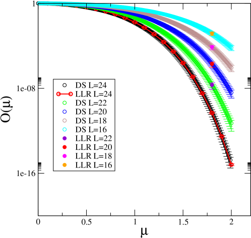
Figure 6: The overlap $O(\mu)$ (17) from a direct Monte-Carlo simulation of the dual theory (DS) and from the LLR approach for several lattice sizes $L^{3}$. $\tau=0.1$, $\kappa=0.01$.

In order to quantify the influence of the imaginary part, we introduce the partition function $Z_{\mathrm{mod}}$ that features the $Z_{3}$ action (4) from which we have dropped the imaginary part:

$$S_{\mathrm{mod}}[z]={\tau}\sum_{x,\nu}[z_{x}z^{\ast}_{x+\nu}+cc]\;+\;\kappa\,\cosh(\mu)\,[2N_{1}\,+\,N_{+}\,+\,N_{-}\,]\;,$$ (16)

where $N_{1}$ is the number of $z=1$ elements on the lattice. The partition function of the modified theory does depend on the chemical potential, but note that it can be simulated by standard Monte-Carlo techniques since its Gibbs factor is real and positive by construction. We then define the overlap between the full theory and the modified theory by

$$O(\mu)=\frac{Z(\mu)}{Z_{\mathrm{mod}}(\mu)}\;.$$ (17)

We point out that being able to calculate the overlap $O(\mu)$ provides access to the observables of the full theory. For instance, the density $\rho(\mu)$ acquires two parts:

$$\rho(\mu)\;=\;\frac{d\,\ln Z(\mu)}{d\mu}\;=\;\frac{d\,\ln O(\mu)}{d\mu}\;+\;\frac{d\,\ln Z_{\mathrm{mod}}(\mu)}{d\mu}\;,$$ (18)

where the latter part is free of a sign problem and is calculable by standard Monte-Carlo simulations.

An appealing feature of the $Z_{3}$ spin model is that its dual is a real theory open for Monte-Carlo simulations. In fact, the theory can be efficiently simulated by a worm type algorithm (see [18]) where the “worms” are conserved flux lines of the dual theory (see [20] for this interpretation). It is still difficult to calculate the partition function itself since theories with different chemical potentials differ in the free energy density $f(\mu)$ leading to poor overlap:

$$\frac{Z(\mu+\Delta\mu)}{Z(\mu)}\;=\;\exp\Bigl{\{}-\,[f(\mu+\Delta\mu)\,-\,f(\mu)]\;V\Bigr{\}}\;.$$ (19)

We used a variant of the “snake algorithm” [32] to calculate ratios of the partition function and to reconstruct the partition function from those:

$$Z(k\,\Delta\mu)\;=\;Z(0)\,\prod_{\ell=1}^{k}\frac{Z(\ell\Delta\mu)}{Z((\ell-1)\Delta\mu)}\;,$$ (20)

where $\Delta\mu$ must be chosen small enough (depending on the number of degrees of freedom $V$) to ensure a good enough signal-to-noise ratio. We here point out an advantage of the LLR approach: $k$ simulations of the dual theories are necessary to arrive at the target value $\mu_{t}\;=\;k\Delta\mu$, while the LLR approach can aim directly at the chemical potential $\mu_{t}$ of interest.

We have simulated the $Z_{3}$ theory with non-zero chemical potentials using the LLR method [30]. We point out that the method is exact implying that the numerical results need to agree within error bars with the exact values. Note, however, that sophisticated techniques for the error analysis (e.g. bootstrap) might be needed and that standard Gaussian error analysis might fail at least in certain regions of parameter space [33]. Our results from the direct simulation (DS) of the dual theory are shown in figure 6 in comparison with our results from the LLR approach. In the latter case, we have used the method of the polynomial fit from subsection 3.1 for the evaluation of the highly oscillating integral. We indeed encounter a strong sign problem since the overlap is as small as $10^{-16}$ for $\mu\approx 2$. So far, we have only explored a limited region of the parameter space $(\tau,\kappa)$, but our results serve as a proof of concept: for a range of volumes and for the case of a strong sign problem, the simulation of the theory in its original degrees of freedom is feasible using the LLR techniques.

5 Conclusions

Quantum field theory at finite density or, more general, statistical systems with complex actions such as the imbalanced Fermi gas [34] still await first principles results from computer simulations. In the latter case, theoretical findings can be scrutinised against experiments, and, given the level of abstraction that went into model building, agreement would signal an understanding of the materials at hand (see e.g. [35]). In the context of QCD at finite baryon densities, a variety of mechanisms have been proposed over the last couple of years that should describe the states of baryon matter in the intermediate temperature and density range with or without a strong magnetic field. Proposals feature “quarkyonic matter” [3], suggested on the basis of the ’t Hooft limit, the “chiral magnetic effect” [4] or the “Fermi-Einstein condensation” of quarks [5], and this is not meant to be a complete list. Lattice simulations would provide a genuine non-perturbative approach with good systematic control of the errors, but are hampered by the notorious sign problem: for a non-vanishing chemical potential, the Gibbs factor is complex (or, at least, not positive definite) and the action based importance sampling, which is at the heart of the Monte-Carlo simulations, are impossible.

Alongside the new theory proposals for the potential state of matter a finite densities, the last decade has seen promising progress for the simulation of theories with a sign problem. In fact, many of the related ideas are rooted in the literature for decades, but techniques have reached an unprecedented level of sophistication. A good example are the Langevin simulation of complex actions systems, which date back to the early works by Parisi [9] and Karsch and Wyld [10] from the mid eighties, but underwent a Renaissance when it was realised the Silver-Blaze problem can be avoided for the case of a relativistic Bose gas [11].

Similarly, the LLR algorithm [1] emerged from a modification of Wang-Landau type algorithms [26] and have progressed along the lines of the so-called density-of-states methods (see e.g. [27] or [37, 38, 39, 40]). The LLR algorithm copes with continuous degrees of freedom and is designed to numerically calculate the probability distribution of an extensive quantity, the action [1] or e.g. the Polyakov line [29], to an unprecedented precision and for regions of the variable (e.g. action) that would never be visited by an action based importance sampling Monte-Carlo approach. Thus, the LLR algorithm naturally solves overlap problems. Given the belief of a correspondence between the overlap and the sign problem in finite density quantum field theory, it was natural to explore its readiness for complex action theories [30]. Here, the LLR algorithm provides a high quality probability distribution for the imaginary part of the action, and the partition function emerges as the Fourier transform of this distribution with the chemical potential as its frequency (see (3)). Details and advances of the LLR methods have e.g. been reported in [1, 28, 33, 30]. In this paper, we have focused on possible techniques to extract an signal, which is exponentially small with the volume, from the highly oscillating Fourier integral. As a proof of concept, we have studied the $Z_{3}$ spin model [30]. For this model, we have used (for a limited range of the parameter space) the Polynomial Fit technique from subsection 3.1. Despite of a severe sign problem (as quantified by a phase factor expectation value at the $10^{−16}$ level; see figure 6), we were able to obtain reliable results by simulating the theory in its original formulation using the LLR techniques. An analysis of the full parameter space of the $Z_{3}$ model, the LLR simulation of more involved theories (e.g. the $O(2)$-model) and the exploration of the techniques outlined in section 3 to carry out the Fourier transform are currently work in progress.

We are indebted to Arieh Iserles for fruitful discussions on highly oscillating integrals. This work is supported by STFC under the DiRAC framework. We are grateful for the support from the HPCC Plymouth, where the numerical computations have been carried out. KL and AR are supported by the Leverhulme Trust (grant RPG-2014-118) and STFC (grant ST/L000350/1). BL is supported by the Royal Society (grant UF09003) and by STFC (grant ST/G000506/1).

References

References

- [1] K. Langfeld, B. Lucini and A. Rago, Phys. Rev. Lett. 109 (2012) 111601 [arXiv:1204.3243 [hep-lat]].
- [2] E. Laermann and O. Philipsen, Ann. Rev. Nucl. Part. Sci. 53 (2003) 163 [hep-ph/0303042].
- [3] L. McLerran and R. D. Pisarski, Nucl. Phys. A 796 (2007) 83 [arXiv:0706.2191 [hep-ph]].
- [4] K. Fukushima, M. Ruggieri and R. Gatto, Phys. Rev. D 81 (2010) 114031 [arXiv:1003.0047 [hep-ph]].
- [5] K. Langfeld and A. Wipf, Annals Phys. 327 (2012) 994 [arXiv:1109.0502 [hep-lat]].
- [6] K. Splittorff and J. J. M. Verbaarschot, Phys. Rev. Lett. 98 (2007) 031601 [hep-lat/0609076].
- [7] Z. Fodor and S. D. Katz, Phys. Lett. B 534 (2002) 87 [hep-lat/0104001].
- [8] Z. Fodor and S. D. Katz, JHEP 0203 (2002) 014 [hep-lat/0106002].
- [9] G. Parisi, Phys. Lett. B 131 (1983) 393.
- [10] F. Karsch and H. W. Wyld, Phys. Rev. Lett. 55 (1985) 2242.
- [11] G. Aarts, Phys. Rev. Lett. 102 (2009) 131601 [arXiv:0810.2089 [hep-lat]].
- [12] G. Aarts, JHEP 0905 (2009) 052 [arXiv:0902.4686 [hep-lat]].
- [13] G. Aarts, E. Seiler and I. O. Stamatescu, Phys. Rev. D 81 (2010) 054508 [arXiv:0912.3360 [hep-lat]].
- [14] G. Aarts, E. Seiler, D. Sexty and I. O. Stamatescu, Phys. Rev. D 90 (2014) 11, 114505 [arXiv:1408.3770 [hep-lat]].
- [15] P. Rossi and U. Wolff, Nucl. Phys. B 248 (1984) 105.
- [16] P. de Forcrand and M. Fromm, Phys. Rev. Lett. 104 (2010) 112005 [arXiv:0907.1915 [hep-lat]].
- [17] J. Bloch, F. Bruckmann and T. Wettig, JHEP 1310 (2013) 140 [arXiv:1307.1416 [hep-lat]].
- [18] Y. D. Mercado, H. G. Evertz and C. Gattringer, Phys. Rev. Lett. 106 (2011) 222001 [arXiv:1102.3096 [hep-lat]].
- [19] D. Banerjee and S. Chandrasekharan, Phys. Rev. D 81 (2010) 125007 [arXiv:1001.3648 [hep-lat]].
- [20] K. Langfeld, Phys. Rev. D 87 (2013) 11, 114504 [arXiv:1302.1908 [hep-lat]].
- [21] N. Prokof’ev and B. Svistunov, Understanding Quantum Phase Transitions, Lincoln D. Carr,ed. Taylor & Francis, Boca Raton, 2010 [arXiv:0910.1393 [cond-mat.stat-mech]].
- [22] B. B. Brandt and T. Wettig, arXiv:1411.3350 [hep-lat].
- [23] Y. Meurice, Y. Liu, J. Unmuth-Yockey, L. P. Yang and H. Zou, arXiv:1411.3392 [hep-lat].
- [24] S. Chandrasekharan, Phys. Rev. D 82 (2010) 025007 [arXiv:0910.5736 [hep-lat]].
- [25] S. Chandrasekharan and A. Li, Phys. Rev. Lett. 108 (2012) 140404 [arXiv:1111.7204 [hep-lat]].
- [26] F. Wang and D. P. Landau, Phys. Rev. Lett. 86 (2001) 2050 [http://arxiv.org/abs/cond-mat/0011174]
- [27] A. Bazavov, B. A. Berg, D. Du and Y. Meurice, Phys. Rev. D 85 (2012) 056010 [arXiv:1202.2109 [hep-lat]].
- [28] R. Pellegrini, K. Langfeld, B. Lucini and A. Rago, arXiv:1411.0655 [hep-lat].
- [29] K. Langfeld and J. M. Pawlowski, Phys. Rev. D 88 (2013) 7, 071502 [arXiv:1307.0455 [hep-lat]].
- [30] K. Langfeld and B. Lucini, Phys. Rev. D 90 (2014) 9, 094502 [arXiv:1404.7187 [hep-lat]].
- [31] G. Aarts, PoS CPOD 2014 (2014) 012 [arXiv:1502.01850 [hep-lat]].
- [32] P. de Forcrand, M. D’Elia and M. Pepe, Phys. Rev. Lett. 86 (2001) 1438 [hep-lat/0007034].
- [33] Y. D. Mercado, P. Törek and C. Gattringer, arXiv:1410.1645 [hep-lat].
- [34] O. Goulko and M. Wingate, PoS LATTICE 2010 (2010) 187 [arXiv:1011.0312 [cond-mat.quant-gas]].
- [35] M. Wingate and O. Goulko, PoS LATTICE 2012 (2012) 057.
- [36] A. Gocksch, Phys. Rev. Lett. 61 (1988) 2054.
- [37] V. Azcoiti, A. Cruz, A. Tarancon and G. Di Carlo, Nucl. Phys. Proc. Suppl. 17 (1990) 727.
- [38] K. N. Anagnostopoulos and J. Nishimura, Phys. Rev. D 66 (2002) 106008 [hep-th/0108041].
- [39] V. Azcoiti, G. Di Carlo, A. Galante and V. Laliena, Phys. Rev. Lett. 89 (2002) 141601 [hep-lat/0203017].
- [40] V. Azcoiti, E. Follana and A. Vaquero, Nucl. Phys. B 851 (2011) 420 [arXiv:1105.1020 [hep-lat]].