Frozen states and active-absorbing phase transitions of the Ising model on networks

Abstract

A zero temperature quench of the Ising model is known to lead to a frozen steady state on random and small world networks. We study such quenches on random scale free networks (RSF) and compare the scenario with that in the Barabási-Albert network (BA) and the Watts Strogatz (WS) addition type network. While frozen states are present in all the cases, the RSF shows an order-disorder phase transition of mean field nature as in the WS model as well as the existence of two absorbing phases separated by an active phase. The WS network also shows an active-absorbing (A-A) phase transition occurring at the known order-disorder transition point. The comparison of the RSF and the BA network results show interesting difference in finite size dependence.

I Introduction

Dynamics on networks is a topic on which extensive works have been done in recent years. Phenomena which have been studied include evolution of spin systems, opinion dynamics, disease spreading dynamics, etc. Barrat ; psen-book . The dynamical picture is quite different from that on regular lattices due to the topological features of network. For example, one can define the dynamics in different ways for the voter model on a network while these rules become identical on lattices caste .

The study of Ising model on networks has revealed a number of interesting features when static properties are considered. Even in one dimension, when randomly new links are added (or existing links rewired) as in a Watts Strogatz (WS) network WS , one gets a phase transition Weigt ; Gitterman ; Niko which occurs with mean field criticality Kim ; Herrero ; Hong . On Euclidean networks, indications of both mean field type and finite dimensional-like phase transitions have been shown to exist by varying the relevant parameter achat-psen . On scale free networks Leone ; Golt ; Igloi , the transition temperature shows a logarithmic increase with the system size which is perhaps the most surprising result Alek ; Bian ; Herrero1 ; Viana .

While considering ordering dynamics on regular lattices at zero temperature for the Ising model using Glauber dynamics, it is known that for any dimension greater than one, freezing occurs with a probability dependent on the dimension redner . This happens when one considers a completely random initial condition. On random graphs and networks, one encounters similar freezing phenomena which depend on the density of added links svenson ; hagg ; boyer ; pratap .

On random networks or graphs, the evolution of the Ising model from a completely random state shows that the system does not order. A freezing effect was observed and although there could be an emergent majority of nodes with either spin up or spin down state, domains of nodes with opposing spins survive svenson ; hagg . Careful observations show that the disordered state is not an absorbing state castellano . It is instead a stationary active state, with some spins flipping, while keeping the energy constant. The number of domains remaining in the system is just two. The qualitative picture is then the same as on regular lattices for $d>2$ redner , the system wanders forever in an iso-energy set of states. The distribution of the steady state residual energy (which is identical to the number of bonds between oppositely oriented spins apart from a constant) for the Ising model on a random networks was investigated baek . It was found that the distribution typically shows two peaks, one very close to the actual ground state where the residual energy is zero and one far away from it.

Dynamics of the Ising model on the WS network with restricted rewiring has also been considered. Here initially a spin is connected to its four nearest neighbours and then only the second nearest neighbour links are rewired with probability $p$. The system therefore always remains connected. Under the zero temperature Glauber dynamics, freezing effect was observed for any $p\neq 0$ biswas .

In this paper, we have considered in detail the variation of the relevant thermodynamic quantities as functions of time for the zero temperature dynamics of Ising model on various networks. Our main emphasis is on the Ising model on scale free networks at temperature $T=0$ as such studies have not been made so far to the best of our knowledge. Apart from the question whether the equilibrium state is reached or not, we have also explored the nature of the state in case it does not. We are interested to see whether any active-absorbing phase transition occurs as the system parameters are varied. Both the random scale free network (RSF) and the Barabási-Albert (BA) network have been considered for the study. Although many results are known for the WS network, we have explored specifically the possibility of an active-absorbing phase transition in this network. The BA model is studied to make direct comparison with the random scale free network, where results can be quite different albert1 . Also, comparison with respect to issues like freezing and absorbing phase transition may be made for the RSF and the WS networks.

In section II, we describe the network models and the dynamical evolution. The quantities which have been calculated are defined in Section III. The results are presented in the next section and in the last section we summarise and discuss the studies made.

II THE NETWORK MODELS and DYNAMICS

We have considered three different types of network: (a) Random scale free, (b) Barabási-Albert and (3) Watts Strogatz (addition type) WS network. We describe in brief how these networks are generated and the dynamical evolution process. In this section we also include a brief discussion of how the numerical data had been analysed in previous studies.

II.1 Random scale free (RSF) network

In the random scale free network the degree distribution follows a power law but otherwise the network is random. To generate random scale free network albert1 ; doro ; boguna ; newman ; albert ; psen , we assigned the degree of each node using the power law:

$${\mathcal{P}}(k)\sim k^{-\gamma},$$ (1)

where $k$ is the degree of node and $\gamma$ is the characteristic degree exponent. The minimum value of $k$ is $1$ and the maximum cut-off value is $\surd N$, where $N$ number of nodes. This cut-off value ensures that there is no correlation cutoff . Starting from the node with the maximum degree, links have been established with randomly selected distinct nodes.

II.2 Barabási-Albert (BA) network

Barabási-Albert network is a growing network where new nodes are joined to existing nodes with preferential attachment. We start with the three fully connected nodes. Subsequently, a single node is added at a time to the network which is linked to one existing node. The probability that the new node is connected to the existing $i$th node with degree $k_{i}$ is given by albert ; albert1 ,

$$\Pi(k_{i})=k_{i}/{\sum_{j}{k_{j}}}.$$ (2)

Degree distribution of the network is a power law with exponent $\gamma=3$; $P(k)\sim k^{-3}$ albert1 .

II.3 Watts Strogatz (addition type) model

Addition type WS network is a one dimensional regular chain with two nearest neighbour links as well as with some extra randomly connected long range links. Here the long range links have been added with probability $q/N$ (total long range links $\sim O(N)$), where $N$ is the number of nodes and $q$ is a parameter, which denotes the number of extra long range links per node on an average. So the average degree per node of this network is $2+q$, which is a finite quantity as $q/N\to 0$ in the thermodynamic limit. It is known Gitterman that an order-disorder transition occurs at $q=1$.

II.4 Dynamics of Ising model on networks

The Hamiltonian of the Ising system in these networks can be expressed as

$$H=-{\sum_{i<j}{J_{ij}S_{i}S_{j}}}\\ ,$$ (3)

where $S_{i}=\pm 1$ and $J_{ij}=1$ when sites $i$ and $j$ are connected and zero otherwise. Starting with the random configuration, single spin flip energy minimizing Glauber dynamics has been used to update the spin. In this dynamics a randomly selected spin is flipped if the energy of the updated configuration is lowered. It is flipped with probability $1/2$ if the energy remains unchanged on flipping. Fifty different network configurations have been considered and for each network hundred different initial configurations have been taken. The results are averaged over these configurations. We have considered system sizes $N$ upto $1600$. Periodic boundary condition has been used for the WS model which is embedded in real space.

Previous studies have shown that for the thermally driven phase transition, not only mean field critical behaviour exists for the Ising model on small world networks but finite size scaling is also valid there Kim ; Herrero ; Hong ; achat-psen . The data collapse was obtained by rescaling the data and the scaling argument occurring in the scaling function was found to be of the familiar form $\epsilon N^{1/\tilde{\nu}}$ (with $\tilde{\nu}=2$) where $\epsilon$ denotes the deviation from the critical point. $\tilde{\nu}$ is argued to be equal to $\nu d$ where $\nu$ is the correlation length exponent and $d$ the effective dimension of the system. With mean field critical exponent $\nu=0.5$, $d$ turns out to be equal to the upper critical dimension; $d=4$.

III Quantities calculated

We have estimated the following quantities in the present work.

1. Magnetisation: $m(t)$ has been calculated by taking the average of the absolute values of the magnetisation, $m={\langle|\sum_{i}S_{i}|\rangle}/{N}$, as a function of time. Since evolution to both up spin dominated and down spin dominated configurations are possible, the absolute value is taken to compute the configuration average. Distribution of saturation value of magnetisation has also been estimated for random scale free (RSF) network.

2. Residual energy: $E_{r}(t)=E(t)-E_{g}$ where $E_{g}$ is the equilibrium energy of the ground state per spin and $E(t)$ the energy per spin at time $t$. Residual energy measurement indicates the closeness to the equilibrium ground state. Since we are employing a zero temperature quench, the equilibrium ground state configuration corresponds to either all spins up or down.

3. $P_{flip}(t)=N_{flip}(t)/N$, where $N_{flip}$ is the number of spin flips at time $t$, has been studied as a function of time. We count all the spin flips, i.e., if the same spin flips more than one time, all these occurrences are taken into account.

4. Freezing probability $F$ is defined as the probability that the system does not reach the true ground state. It has been calculated as a function of the relevant parameters. For $T=0$, the known ground state is the ferromagnetic state with $m(t\rightarrow\infty)=1$. A frozen configuration will have an absolute value of magnetisation less than $1$.

5. Whether or not the dynamics continue, the system always reaches an iso-energy state. Time $\tau$ to reach the iso-energy state has been calculated as a function of the relevant parameter for random scale free (RSF) network.

The saturation values have been denoted using appropriate subscript, e.g. $m_{sat}$ for magnetisation.

IV Results

IV.1 Random scale free network

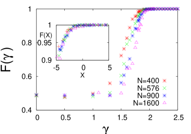
Figure 1: (Color online) RSF: Variation of freezing probability $F(\gamma)$ as a function of $\gamma$ for different system size $N$. Inset shows the data collapse where $F(\gamma)$ has been plotted against $X=(\gamma-\gamma_{c}^{f})N^{1/{\tilde{\nu}}}$.

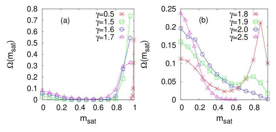
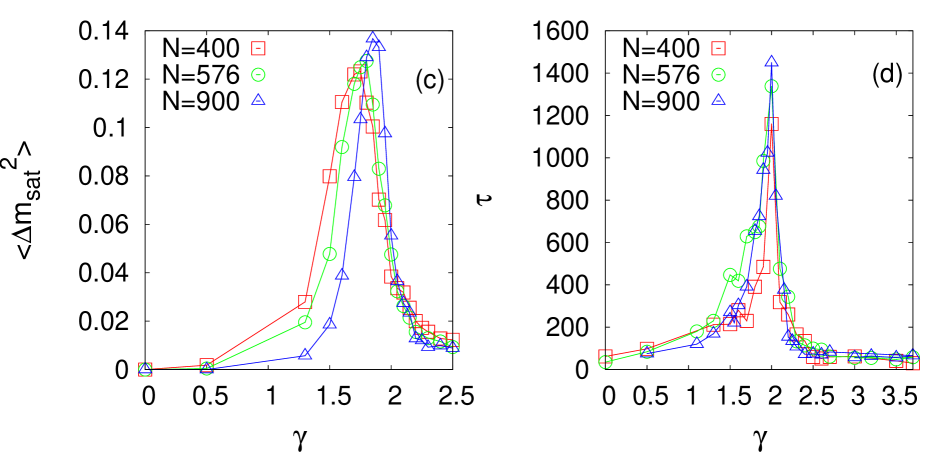
Figure 2: (Color online) RSF: ((a), (b)) The distribution of saturation value of magnetisation for $N=576$ for different values of $\gamma$. (c) The variation of fluctuation of saturation value of magnetisation and (d) time to reach the energetically stable state as a function of $\gamma$ for different system size $N$.

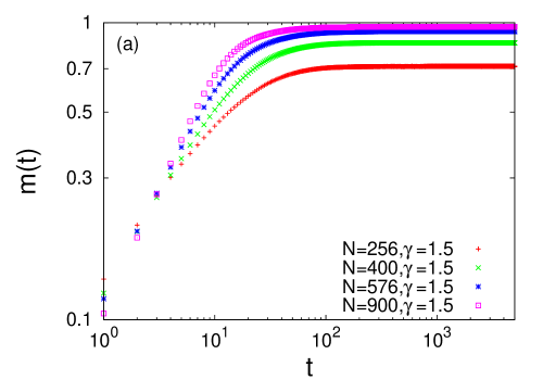
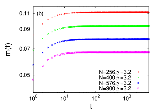
Figure 3: (Color online) RSF: Variation of magnetisation $m(t)$ with time for different system size $N$. (a) $\gamma=1.5$ and (b) $\gamma=3.2$.

We first discuss the behaviour of the freezing probability $F$ on the RSF. The variation of $F$ with the network parameter $\gamma$ for different system sizes suggests that a freezing transition takes place here as the freezing probability is unity above a value of $\gamma$ which we denote by $\gamma_{c}^{f}$ (Fig. 1). Of course, if the initial state is fully ordered it is not counted as a frozen state. However, barring these two states (all up/ all down), none of the other initial states reaches the actual equilibrium configuration. Hence the freezing probability is actually $1-2/2^{N}$ which becomes unity in the thermodynamic limit. Below $\gamma_{c}^{f}$, the freezing probability decreases with system size and shows a system size independent behaviour for $\gamma\lesssim 1.0$. The freezing probability is non zero for all values of $\gamma$.

As the freezing probability shows finite size dependence close to $\gamma_{c}^{f}$ and since it is dimensionless, we argue that it should show a finite size scaling behavior in the following manner

$$F(\gamma,N)=g_{1}[(\gamma-\gamma_{c}^{f})N^{1/{\tilde{\nu}}}]$$ (4)

where $g_{1}$ is a scaling function. We estimate $\gamma_{c}^{f}\approx 2.0$ and the exponent $\tilde{\nu}\approx 2.20$ (inset of Fig.1). The estimates are obtained from the manifestly best collapse of the data after rescaling is done properly. As already discussed in section II.4, finite size scaling is valid for the Ising model on networks with $\tilde{\nu}=\nu d$ where $\nu$ is the mean field value of the correlation length exponent and $d$ is equal to $4$. Assuming the same to hold good here, we get $\nu\approx 0.55$ from the fact that $\tilde{\nu}\approx 2.2$ which is fairly close to the mean field value $0.5$ for Ising model Stanley .

We next show that an order-disorder phase transition also occurs in this network. The distribution of magnetisation $\Omega(m_{sat})$ has been studied (Fig. 2a, b). It is unimodal in nature for the values of $\gamma$ far from the $\gamma_{c}^{f}$. The peaks occur at $m_{sat}\sim 1$ for $\gamma\ll\gamma_{c}^{f}$ and $m_{sat}\sim 0$ for $\gamma\gg\gamma_{c}^{f}$. The distribution is bimodal close to $\gamma_{c}^{f}$ with the peak values at $m_{sat}\sim 0$ and $m_{sat}\sim 1$.

Fluctuations of the saturation value of the magnetisation $\langle{{\Delta{m_{sat}}^{2}}}\rangle$ shows a peak which shifts toward $\gamma_{c}^{f}$ and the the peak value increases as the system size is increased (Fig. 2c). We have also estimated the time $\tau$ to reach the energetically stable state. It shows a peak close to $\gamma_{c}^{f}$. Clearly $\tau$ diverges near $\gamma_{c}^{f}$, as the peak value increases with system size (Fig. 2d). These behaviour suggest that there is an order-disorder transition also taking place as $\gamma$ is varied. In principle the order-disorder transition may take place at a value $\gamma_{c}^{m}\neq\gamma_{c}^{f}$ and we make further analysis to estimate $\gamma_{c}^{m}$ more accurately. We also check whether a mean field-like behaviour is present for the order-disorder transition.

The variation with time of the magnetisation $m(t)$ has been shown for different system sizes for two different values of the degree exponent $\gamma$ (Fig. 3a, b). The behaviour of the saturation values of the magnetisation $m_{sat}$ for finite sizes shows the typical characteristics of a continuous phase transition with $\gamma$ acting as the driving parameter (Fig. 4).

Using finite size scaling method we indeed obtain a collapse of the data points for $m_{sat}$ for different system sizes. The following scaling form for $m_{sat}$ has been used:

$$m_{sat}=N^{-\beta/{\tilde{\nu}}}g_{2}[(\gamma-\gamma_{c}^{m})N^{1/{\tilde{\nu}}}]\\ .$$ (5)

We obtain $\gamma_{c}^{m}\approx 2.20$, $\beta\simeq 0.47$ and $\tilde{\nu}\simeq 2.20$ (inset of Fig. 4). The values of the exponents $\beta$ and $\nu$ are fairly close to the mean field values once again.

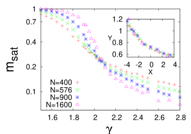
Figure 4: (Color online) RSF: Variation of saturation value of magnetisation as a function of $\gamma$ for different system size $N$. Inset shows the data collapse where $Y=m_{sat}N^{\beta/{\tilde{\nu}}}$ has been plotted against $X=(\gamma-\gamma_{c}^{m})N^{1/{\tilde{\nu}}}$.

Next we discuss the behaviour of the residual energy and the spin flip probability which also attain a saturation value in time ($P_{sat}$ and $E_{sat}$). Both the saturation values $P_{sat}$ and $E_{sat}$ show nonmonotonic variation with $\gamma$ (Figs. 5, 6), with a peak which shifts as the system size is increased. $P_{sat}$ in particular shows a very interesting behaviour with finite size. For $\gamma\lesssim 2.0$, it decreases with system size indicating an absorbing phase which is actually the ordered phase as indicated by the behaviour of the magnetisation discussed above. However, there is a region between $\gamma\approx 2.0$ and $\gamma\approx 3.0$, where $P_{sat}$ increases with system size which indicates an active state. For $\gamma\gtrsim 3.0$, $P_{sat}$ decreases with system size indicating an absorbing state once again. Hence we have two absorbing phases separated by an active phase and two transitions as the parameter $\gamma$ is varied. This is reminiscent of two distinct transitions observed in opinion dynamics models droz ; khaleque .

We found from the above studies that $\gamma_{c}^{f}\approx 2.0$ and $\gamma_{c}^{m}\approx 2.2$ are close but not exactly the same. However, this could be due to finite size effects and these two might turn out to be identical, i.e., $\gamma_{c}^{f}=\gamma_{c}^{m}=2.0$ in the thermodynamic limit. This possibility is supported by the behaviour of both $\tau$ and $E_{sat}$. While $\tau$ diverges at $\gamma\simeq 2.0$, $E_{sat}$ decreases with system size below $\gamma\simeq 2.0$ (indicating an order phase) and increases or remains constant above this value (Figs. 6).

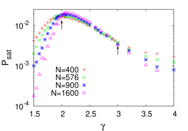
Figure 5: (Color online) RSF: Variation of saturation value of the fraction of spin flips as a function of $\gamma$ for different system size $N$. The vertical arrows separate different phases.

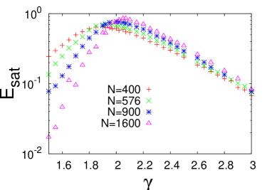
Figure 6: (Color online) RSF: Variation of saturation value of the residual energy as a function of $\gamma$ for different system size $N$.

IV.2 Barabási-Albert network

The BA network has no intrinsic parameter. We calculate the relevant dynamic quantities for different system sizes. The magnetisation $m(t)$ slowly increases for the first few time steps and gets saturated at long times for all the system sizes. Both $E_{r}(t)$ and $P_{flip}(t)$ decrease with time and then reach a saturation value. Saturation values of all these quantities as a function of system size have been plotted in Fig. 7a. The saturation value of magnetisation $m_{sat}(N)$ decreases with system size and the variation shows a power law behaviour. We fitted the variation with the form $m_{sat}(N)=a_{m}N^{-b_{m}}$ and the estimated exponents are $a_{m}\approx 1.467$ and $b_{m}\approx 0.150$.

We have also studied the variation of saturation value of the fraction of spin flips $P_{sat}(N)$ and saturation value of residual energy $E_{sat}(N)$. Both of them show a slowly increasing behaviour with system size and these increasing behaviour also follow power law (Fig. 7a). We fitted the variation of $P_{sat}(N)$ with the form $P_{sat}(N)=a_{f}N^{b_{f}}$ and the exponents are $a_{f}\approx 0.001$ and $b_{f}\approx 0.346$. For $E_{sat}(N)$, the fitted form is $E_{sat}(N)=a_{E}N^{b_{E}}$ and the exponents are $a_{E}\approx 0.083$ and $b_{E}\approx 0.293$. The important point to note here is this seems to be an active phase as the saturation value of the fraction of spin flips shows increase with system size. In contrast, the same quantities plotted for the RSF with $\gamma=3.0$ (Fig. 8) shows that it is an absorbing phase (as already noted in the previous subsection). We will discuss more about this observation in Section V. The variation of $E_{sat}(N)$ with $N$ in RSF is however, similar, with $E_{sat}(N)=0.013N^{0.279}$. $m_{sat}(N)$ for RSF decays as $1.17N^{-0.408}$ which signifies a faster decay compared to the BA network. .

In the BA model, the freezing probability $F(N)$ increases with system size (Fig. 7b). Freezing probability $\rightarrow 1$ for $N\rightarrow\infty$. Thus the BA model is in an active disordered state where none of the configuration reaches the equilibrium ground state. The variation of $F(N)$ with system size fits well with the form $F(N)=1-e^{-a_{d}N^{b_{d}}}$ and the calculated exponents are $a_{d}\approx 0.113$ and $b_{d}\approx 0.548$. The behaviour of the freezing probability as a function of $N$ is also quite different for the BA and the RSF networks (with $\gamma=3$), in the latter we found a system size independent behaviour.

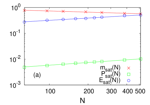
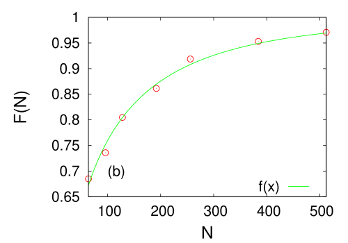
Figure 7: (Color online) BA: (a) Variation of saturation value of magnetisation $m_{sat}(N)$, fraction of spin flips $P_{sat}(N)$ and residual energy $E_{sat}(N)$ as a function system size. (b) Variation of freezing probability $F(N)$ as a function of system size $N$.

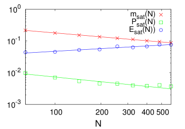
Figure 8: (Color online) RSF($\gamma=3.0)$: Variation of saturation value of magnetisation $m_{sat}(N)$, fraction of spin flips $P_{sat}(N)$ and residual energy $E_{sat}(N)$ as a function system size.

IV.3 WS network

On the WS network, all the relevant quantities show a saturation behaviour as already noted previously on a slightly different version of the WS network biswas .

Here in addition, we have studied the spin flip probabilities. The saturation value of the probability of spin flips $P_{sat}$ has been plotted against the parameter $q$ for different system sizes and this quantity reveals interesting behaviour (Fig. 9a). It is clearly seen that above $q\simeq 1$, the probability decreases as a function of system size $N$ while below $q\simeq 1$ it is almost size independent. This indicates that there is an active absorbing phase transition taking place at this point.

The value of the freezing probability $F(q)$ either increases with $N$ or remains constant which clearly shows that the entire phase is frozen for any $q>0$. We find that for $q<1$ the freezing probability reaches unity in the thermodynamic limit while it remains fairly constant beyond this value (Fig. 9b). This is consistent with the active-absorbing phase transition stipulated to take place at $q=1$; in the active state, one can never reach the equilibrium ground state configuration.

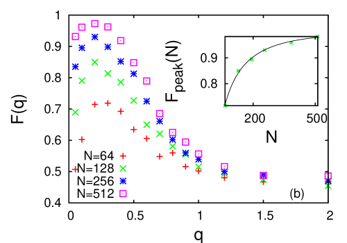
Figure 9: (Color online) WS: Variation of (a) saturation value of fraction of spin flips $P_{sat}$ and (b) freezing probability $F(q)$ as a function of $q$ for different system sizes $N$ (right panel). Inset of (b) shows the variation of peak value of $F(q)$ with the system size.

$F(q)$ shows a peak at $q=0.2$ and the position of the peak is independent of system size which shows that the system is maximally disordered here. The peak values of freezing probability as a function of system size $N$ is fitted with the form $F_{peak}(N)=1-e^{-aN^{b}}$ and the estimated values of the exponents are $a\approx 0.134$ and $b\approx 0.540$ (inset of Fig. 9b). It may be noted that the same form is obeyed in the BA model.

V Discussions and conclusions

We have studied zero temperature Glauber dynamics of the Ising model on three types of networks and compared the results. Frozen state is observed in all the three types of network models. For random scale free network, freezing probability is unity for $\gamma\gtrsim 2$, i.e., the system never reaches the global equilibrium but for lower value of the parameter $\gamma$, it decreases with system size and shows a system size independent behaviour for $\gamma\lesssim 1$. This behaviour of freezing probability suggests a freezing transition point at $\gamma_{c}^{f}\simeq 2.0$. We also find an order disorder transition point taking place very close to this point; in fact we believe that they occur at the same point and the difference is only a finite size effect. Also close to this point, the first active-absorbing (A-A) phase transition takes place; the disordered phase for $2\lesssim\gamma\lesssim 3$ is active while for $\gamma\lesssim 2$, one gets an absorbing phase. A second A-A transition takes place close to $\gamma\approx 3.0$ and the system evolves to an absorbing disordered state beyond this value. In all probability these two A-A transitions take place at $\gamma=2.0$ and $3.0$ in absence of finite size effects; these two points are significant as for $\gamma\leq 2.0$, the average degree diverges while for $\gamma\leq 3.0$, the degree variance diverges in the thermodynamic limit.

One can compare the results of RSF network and BA network for the same characteristic degree exponent $\gamma=3.0$. The residual energy shows an increase with system size $N$ in both cases in a power law manner with an exponent which is fairly close. Also, the saturation value of magnetisation decreases with $N$ in both networks in a power law manner, corresponding exponents are however quite different. The saturation energy and magnetisation behaviour are consistent with the fact that the state is disordered for both RSF and BA networks. However freezing probability for BA model and RSF network show different behaviour with system size. For RSF, the freezing probability shows a system size independent behaviour while for BA model, it has a nonlinear dependence. As far as the spin flip probability is concerned RSF (at $\gamma=3.0$) again differs from the BA network. The RSF network and BA model are intrinsically different, BA is a growing network generated with a particular strategy. There is no loop in this network. In the case of RSF, the structure is completely different, there may be loops. Although in a numerical study, the value of $\gamma$ may not be exactly 3 in either the RSF or BA networks due to finite size effects, we believe that this cannot be the reason for the results being qualitatively different. In fact previous studies on RSF and BA have shown that characteristic features may be quite different for the two networks albert1 ; psen .

The results obtained for the WS model can also be compared to those found for the RSF network and BA network. In the WS network an A-A transition is observed at $q\simeq 1.0$ which is also the order-disorder transition point. Hence this is similar to the occurrence of an A-A and an order-disorder transition occurring simultaneously in the RSF. However in the WS network, the entire disordered phase is active. For small average degree the system is in an active and for large degree in an absorbing phase. For the RSF network, two A-A transitions exist where absorbing phase is observed for both large degree and small degree and an active state exists in between these two absorbing phases. In both RSF and WS another interesting feature is present, the ordered state shows a finite freezing probability with negligible system size dependence. In the WS network maximum value of the freezing probability $F(q)$ occurs at $q\approx 0.2$ and shows a behaviour similar to the freezing probability in BA network as a function of system size.

To summarise, a systematic study of ordering dynamics of the Ising model on scale free networks has been made for the first time to the best of our knowledge. It is observed that the system freezes to a non equilibrium steady state for all values of the relevant parameters in the random scale free networks (RSF) and the Barabási-Albert model (BA). The presence of two active-absorbing phase transitions in the RSF makes it different from the WS network where only one such transition is observed. It is also concluded that in RSF one of the active-absorbing phase transition takes place at the order-disorder transition point which is similar to what is observed in the WS network.

Acknowledgements: The authors thank Soham Biswas for his suggestions and encouragement. AK acknowledges financial support from UGC sanction no. F.7-48/2007(BSR). PS acknowledges financial support from CSIR project. Computations made on HP cluster financed by DST (FIST scheme), India.

References

- (1) A. Barrat and M. Barthelemy and A. Vespignani, Dynamical Processes on Complex Networks, Cambridge University Press, 2008.
- (2) P. Sen and B. K. Chakrabarti, Sociophysics: An Introduction, Oxford University Press, 2013.
- (3) C. Castellano, S. Fortunato and V. Loreto, Rev. Mod. Phys. 81 591 (2009).
- (4) D. J. Watts and S. H. Strogatz, Nature 393 440 (1998).
- (5) A. Barrat and M. Weigt, Eur. Phys. J. B 13, 547 (͑2000͒).
- (6) M. Gitterman, J. Phys. A : Math. Gen. 33 8373 (2000).
- (7) T. Nikoletopoulos, A. C. C. Coolen, I. Prez Castillo, N. S. Skantzos, J. P. L. Hatchett and B. Wemmenhove, J. Phys. A 37, 6455 (͑2004͒).
- (8) B. J. Kim, H. Hong, P. Holme, G. S. Jeon, P. Minnhagen and M. Y. Choi, Phys. Rev. E 64 056135 (2001).
- (9) C. P. Herrero, Phys. Rev. E 65 066110 (2002).
- (10) H. Hong, B. J. Kim and M. Y Choi, Phys. Rev. E 66 011107 (2002).
- (11) A. Chatterjee and P. Sen, Phys. Rev. E 74 036109 (2006).
- (12) M. Leone, A. VÁzquez, A. Vespignani, and R. Zecchina, Eur. Phys. J. B 28, 191 (2002).
- (13) S. N. Dorogovtsev, A. V. Goltsev, and J. F. F. Mendes, Phys. Rev. E 66, 016104 (2002).
- (14) F. Iglói and L. Turban, Phys. Rev. E 66, 36140 (2002).
- (15) A. Aleksiejuk, J. A. Holyst and D. Stauffer, Physica A 310 260 (2002).
- (16) G. Bianconi, Phys. Lett. A 303 166 (2002).
- (17) C. P. Herrero, Phys. Rev. E . 69 067109 (2004).
- (18) J. Viana Lopes, Yu. G. Pogorelov, J. M. B. Lopes dos Santos and R. Toral, Phys. Rev. E 70 026112 (2004).
- (19) V. Spirin, P. L. Krapivsky and S. Redner, Phys. Rev. E 63 036118 (2001).
- (20) P. Svenson, Phys. Rev. E 64 036122 (2001).
- (21) O. Haggstrom, Physica A 310 275 (2002).
- (22) D. Boyer and O. Miramontes, Phys. Rev. E 67 R035102 (2003).
- (23) P. K. Das and P. Sen, Eur. Phys. J. B 47 391 (2005).
- (24) C. Castellano, V. Loreto, A. Barrat, F. Cecconi and D. Parisi, Phys. Rev. E 71 066107 (2005).
- (25) Y. Baek, M. Ha and H. Jeong, Phys. Rev. E 85 031123 (2012).
- (26) S. Biswas and P. Sen, Phys. Rev. E 84 066107 (2011).
- (27) R. Albert and A. L. Barabási, Rev. Mod. Phys. 74 47 (2002).
- (28) R. Albert and A. L. Barabási, Science, 286, 509 (1999).
- (29) S. N. Dorogovtsev and J. F. F. Mendes, Evolution of Networks: From biological nets to the Internet and WWW, ̵͑Oxford University Press, Oxford, 2003͒.
- (30) M. Boguñá, R. Pastor-Satorras and A. Vespignani, Eur. Phys. J. B 38, 205 (2004).
- (31) M. E. J. Newman, Networks: An Introduction (Oxford University Press, 2010).
- (32) P. Sen, Journal of Statistical Mechanics P04007 (2007).
- (33) M. Catanzaro, M. Boguñá and R. Pastor-Satorras, Phys. Rev. E 71 027103 (2005).
- (34) H. E. Stanley, Introduction to phase transitions and critical phenomena (Oxford University Press, Jul 1987͒).
- (35) M. Droz, A. L. Ferreira and A. Lipowski, Phys. Rev. E 67 056108 (2003).
- (36) A. Khaleque and P. Sen, Physica A 413 599 (2014).