Vector Fitting for Matrix-valued Rational Approximation

Abstract

Vector Fitting (VF) is a popular method of constructing rational approximants that provides a least squares fit to frequency response measurements. In an earlier work, we provided an analysis of VF for scalar-valued rational functions and established a connection with optimal $\mathcal{H}_{2}$ approximation. We build on this work and extend the previous framework to include the construction of effective rational approximations to matrix-valued functions, a problem which presents significant challenges that do not appear in the scalar case. Transfer functions associated with multi-input/multi-output (MIMO) dynamical systems typify the class of functions that we consider here. Others have also considered extensions of VF to matrix-valued functions and related numerical implementations are readily available. However to our knowledge, a detailed analysis of numerical issues that arise does not yet exist. We offer such an analysis including critical implementation details here.

One important issue that arises for VF on matrix-valued functions that has remained largely unaddressed is the control of the McMillan degree of the resulting rational approximant; the McMillan degree can grow very high in the case of large input/output dimensions. We introduce two new mechanisms for controlling the McMillan degree of the final approximant, one based on alternating least-squares minimization and one based on ancillary system-theoretic reduction methods. Motivated in part by our earlier work on the scalar VF problem as well as by recent innovations for computing optimal $\mathcal{H}_{2}$ approximation, we establish a connection with optimal $\mathcal{H}_{2}$ approximation, and are able to improve significantly the fidelity of VF through numerical quadrature, with virtually no increase in cost or complexity. We provide several numerical examples to support the theoretical discussion and proposed algorithms.

1 Introduction

Rational functions provide significant advantages over other classes of approximating functions, such as polynomials or trigonometric functions, that are important in the approximation of functions that occur in engineering and scientific applications. Matrix-valued rational functions offer substantial additional flexibility and broaden the domain of applicability by providing the potential for the interpolation and approximation of parameterized families of multi-dimensional observations. For example, in a variety of engineering applications, the dynamics arising from multi-input/multi-output (MIMO) dynamical systems may be inaccessible to direct modeling, yet input-output relationships often may be observed as a function of frequency, yielding an enormous amount of data. In such cases, one may wish to deduce an empirical dynamical system model nominally represented as a matrix-valued rational function, that fits the measured frequency response data. This derived model may then be used as a surrogate in order to predict system behavior or to determine suitable control strategies. See [2, 8, 53] for examples of rational approximation in action.

The McMillan degree of a matrix-valued rational function, ${\mathbf{H}}(s)$, is the sum of pole multiplicities over the (extended) complex plane, or equivalently, the dimension of the state space in a minimal realization of ${\mathbf{H}}(s)$. It is convenient to think of ${\mathbf{H}}(s)$ as a transfer function matrix associated with a stable MIMO linear time-invariant system having $m$ inputs and $p$ outputs (although this interpretation is not necessary for what follows); McMillan degree is a useful proxy for the level of complexity associated with ${\mathbf{H}}(s)$. Let $r>0$ be an integer denoting the desired McMillan degree for our approximant: ${\mathbf{H}}_{r}(s)={\mathbf{N}}(s)/d(s)$, where ${\mathbf{N}}(s)$ is a $p\times m$ matrix having elements that are polynomials in $s$ of order $r-1$ or less, and $d(s)$ is a (scalar) polynomial function having exact order $r$. Denote by $\mathcal{R}_{r}$ the set of matrix-valued functions of this form. Note that $\mathcal{R}_{r}$ consists of matrix-valued functions having entries that are strictly proper rational functions of order $r$; the McMillan degree of ${\mathbf{H}}_{r}\in\mathcal{R}_{r}$ could range as high as $r\cdot\min(m,p)$, which could be significantly larger than our target, $r$. We assume that observations (evaluations) of ${\mathbf{H}}(s)$ are available at predetermined points in the complex plane, $s=\xi_{1},\,\ldots,\,\xi_{\ell}$. Only observed values at these points: ${\mathbf{H}}(\xi_{j})$, for $j=1,\ldots,\ell$, will be necessary in order to derive our approximations. We proceed by seeking a solution to

$$\min_{{\mathbf{H}}_{r}\in\mathcal{R}_{r}}\sum_{i=1}^{\ell}\rho_{i}\left\|{\mathbf{H}}_{r}(\xi_{i})-{\mathbf{H}}(\xi_{i})\right\|_{F}^{2}\;.$$ (1.1)

Sanathanan and Koerner [52] proposed an approach to solving (1.1) that produces a sequence of rational matrix approximants ${\mathbf{H}}_{r}^{(k)}(s)$ having the form ${\mathbf{H}}_{r}^{(k)}(s)={\mathbf{N}}^{(k)}(s)/d^{(k)}(s)$, where ${\mathbf{N}}^{(k)}(s)$ is a $p\times m$ matrix of polynomials of degree $r-1$ or less and $d^{(k)}(s)$ is a (scalar-valued) polynomial of degree $r$. For each $k$, the coefficients of ${\mathbf{N}}^{(k)}$ and $d^{(k)}$ are adjusted by solving a weighted linear least squares problem with a weight determined by $d^{(k-1)}$. An important reformulation of the Sanathanan-Koerner (SK) iteration was introduced by Gustavsen and Semlyen [36], which became known under the name Vector Fitting (VF). The term “vector fitting” is appropriate in light of the interpretation of the Frobenius norm, $\|\cdot\|_{F}$, that appears in (1.1) as a standard Euclidean vector norm, $\|\cdot\|_{2}$, of an ‘unraveled’ matrix listed column-wise as a vector in ${\mathbb{C}}^{mp}$. The Gustavsen-Semlyen VF method produces a similar sequence of rational approximants ${\mathbf{H}}_{r}^{(k)}(s)={\mathbf{N}}^{(k)}(s)/d^{(k)}(s)$ but now with ${\mathbf{N}}^{(k)}$ and $d^{(k)}$ defined as rational functions represented in barycentric form. Making central use of a clever change of representation at each step, the Gustavsen-Semlyen VF method achieves greater numerically stability and efficiency than the original Sanathanan-Koerner iteration.

We describe both the SK and VF iteration in §2 and make some observations that contribute to our analysis of it in §3. In particular, we note that the change of representation implicit in the VF iteration can be related to a change of representation from barycentric to pole–residue form. This change of representation is made explicit in §2.2, where we provide formulas that appear to be new. These formulas can be useful at any step of either the SK or VF iteration in order to estimate the contribution that each pole makes to the current approximation. This, in turn, is useful in determining whether, $r$, the initial estimate of McMillan degree, is unnecessarily large relative to the information contained in the observed data. We note that many authors have applied, modified, and analyzed VF, see e.g. [35], [38], [20], [19], [22], [21], [23]. A matlab implementation vecfit3 is provided at [54] and is widely used. When applied to MIMO problems, high fidelity rational approximations are sought and generally achieved at the expense of a relatively high McMillan degree for the final approximant. By way of contrast, the approaches we develop here are capable of providing systematic estimates to the McMillan degree of the original function, ${\mathbf{H}}(s)$, and can produce high fidelity rational approximations of any desired McMillan degree, to the extent possible.

In §3, we analyze VF within a numerical linear algebra framework and discuss several important issues that are essential for a numerically sound implementation of the method. Although VF is based on successive solution of least squares (LS) problems, which is a well understood procedure, subtleties enter in the VF context. We review commonly used numerical LS solution procedures in §3.1 and point out some details that become significant in the VF setting. In §3.2, we argue and illustrate by way of example that, as iterations proceed, the VF coefficient matrices in the pole identification phase tend to become noisy with a significant drop in column norms that can also coincide with a reduction in numerical rank. This prompts us to advise caution when rescaling columns in order to improve the condition number, since rescaling columns that have been computed through massive cancellations will preclude inferring an accurate numerical rank.

Ill-conditioning is intrinsic to rational approximation and manifested through the potentially high condition numbers of Cauchy matrices that naturally arise. We introduce in §3.4.2 another approach toward curbing ill-conditioning. Using recent results on high accuracy matrix computations, we show that successful computation is possible independent of the condition number of the underlying Cauchy matrix, and we open possibilities for application of Tichonov regularization and the Morozov discrepancy principle, which provide additional useful tools when working with noisy data. In §3.5, we offer some suggestions for efficient software implementation and provide some algorithmic details that reduce computational cost. For the sake of brevity, we omit discussion of the algorithmic details that allow computation to proceed using only real arithmetic.

Typically, the weights in (1.1) are $\rho_{i}=1$ and the sample points, $\xi_{i}$, are either uniformly or logarithmically spaced according to sampling expedience. We do consider this case in detail, but also propose, in §4, an alternate strategy for choosing $\rho_{i}$ and $\xi_{i}$ that is guided by numerical quadrature. This connects the “vector fitting” process with optimal $\mathcal{H}_{2}$ approximation and follows up on our recent work, [26]. Indeed, with proper choice of the nodes $\xi_{i}$ and the weights $\rho_{i}$, we can interpret the weighted LS approximation of (1.1) as rational approximation in a discretized $\mathcal{H}_{2}$ norm in the Hardy space of matrix functions that are analytic in the open right half-plane. This leads to a significant improvement in the performance of the VF approximation and also sets the stage for a new post-processing stage proposed in §5, where we address the question of computing an approximation having predetermined McMillan degree.

Rational data fitting has a long history (going back at least to Kalman [42]) and continues to be studied in a variety of settings: For example, Gonnet, Pachón, and Trefethen [31] recently provided a robust approach to rational approximation through linearized LS problems on the unit disk. Hokanson in [40] presented a detailed study of exponential fitting, which is closely related to rational approximation. The Loewner framework developed by Mayo and Antoulas [46, 44] is an effective and numerically efficient method to construct rational interpolants directly from measurements. This approach also has been extended successfully to parametric [6, 41] and weakly nonlinear [3, 4] problems. In this paper, we focus solely on matrix-valued rational least-squares approximation by VF.

2 Background and Problem Setting

VF iteration is built upon the Sanathanan–Koerner (SK) procedure [52], which we describe briefly as follows: A sequence of approximations having the form ${\mathbf{H}}_{r}^{(k)}={\mathbf{N}}^{(k)}(s)/d^{(k)}(s)\in\mathcal{R}_{r}$, is developed by taking $d^{(0)}(s)\equiv 1$, and then solving successively for ${\mathbf{N}}^{(k+1)}$ and $d^{(k+1)}$ via the weighted linear least squares problem:

$$\epsilon^{(k)}=\displaystyle\sum_{i=1}^{\ell}\frac{\rho_{i}}{|d^{(k)}(\xi_{i})|^{2}}\left\|{{\mathbf{N}}^{(k+1)}(\xi_{i})-d^{(k+1)}(\xi_{i}){\mathbf{H}}(\xi_{i})}\right\|_{F}^{2}\longrightarrow\min.\;\ \mbox{ for }k=0,1,2,\ldots$$ (2.1)

Since ${\mathbf{N}}^{(k)}$ and $d^{(k)}$ have a presumed affine dependence on parameters, (2.1) does indeed define a linear least squares problem with respect to those parameters. Notice also that once ${\mathbf{N}}^{(k+1)}(s)$ and $d^{(k+1)}(s)$ have been computed, only $d^{(k+1)}(s)$ is used in the next iteration as a new weighting function. Although convergence of this process remains an open question, if the iterations do converge at least in the sense that, at some $k_{*}$, $d^{(k_{*}+1)}(s)$ “is close to” $d^{(k_{*})}(s)$ at the sample points $\xi_{i}$, the process is halted and we take ${\mathbf{H}}_{r}(s)={\mathbf{N}}^{(k_{*}+1)}(s)/d^{(k_{*}+1)}(s)$. Note also that before this last step (i.e., for $k<k_{*}$), any effort to compute the value of ${\mathbf{N}}^{(k+1)}$ is wasted.

The error in (2.1) may be rewritten as $\epsilon^{(k_{*})}=\sum_{i=1}^{\ell}\rho_{i}\left|d^{(k_{*}+1)}(\xi_{i})/d^{(k_{*})}(\xi_{i})\right|^{2}\left\|{{\mathbf{H}}_{r}(\xi_{i})-{\mathbf{H}}(\xi_{i})}\right\|_{F}^{2},$ which corresponds to (1.1) up to an error that depends on the deviation of $|d^{(k_{*}+1)}/d^{(k_{*})}|$ from $1$. This deviation becomes small as convergence occurs and can be associated with stopping criteria that we introduce in §3.4.3. If the iteration is halted prematurely, then the last step leaves $d^{(k)}$ unchanged and redefines ${\mathbf{N}}^{(k+1)}$ as the solution to the LS problem $\sum_{i=1}^{\ell}\rho_{i}\|{\mathbf{N}}^{(k+1)}(\xi_{i})/d^{(k)}(\xi_{i})-{\mathbf{H}}(\xi_{i})\|_{F}^{2}\rightarrow\min$. The implementation of this procedure depends on specific choices for the parameterization of ${\mathbf{N}}^{(k)}(s)$ and $d^{(k)}(s)$ used in representing ${\mathbf{H}}_{r}^{(k)}(s)$; barycentric representations will offer clear advantage.

2.1 VF=SK+barycentric representation

Suppose that at the $k$th iteration step, we choose a set of $r$ mutually distinct (but otherwise arbitrary) nodes, $\{\lambda_{j}^{(k)}\}_{j=1}^{r}$. Consider a barycentric representation for ${\mathbf{H}}_{r}^{(k)}(s)$:

$${\mathbf{H}}_{r}^{(k)}(s)=\frac{{\mathbf{N}}^{(k)}(s)}{d^{(k)}(s)}\equiv\frac{\sum_{j=1}^{r}{\boldsymbol{\Phi}}_{j}^{(k)}/(s-\lambda_{j}^{(k)})}{1+\sum_{j=1}^{r}\varphi_{j}^{(k)}/(s-\lambda_{j}^{(k)})},\;\;{\boldsymbol{\Phi}}_{j}^{(k)}\in\mathbb{C}^{p\times m},\;\;\varphi_{j}^{(k)},\lambda_{j}^{(k)}\in\mathbb{C}.$$ (2.2)

Observe that if $\varphi_{j}^{(k)}\neq 0$, ${\mathbf{H}}_{r}^{(k)}(\lambda_{j}^{(k)})={{\boldsymbol{\Phi}}_{j}^{(k)}}/{\varphi_{j}^{(k)}}$. On the other hand, if $\varphi_{j}^{(k)}=0$ then ${\mathbf{H}}_{r}^{(k)}(s)$ has a simple pole at $\lambda_{j}^{(k)}$ with an associated residue given explicitly in (2.9) of Proposition 1.

A new approximant is sought having the form,

$${\mathbf{H}}_{r}^{(k+1)}(s)=\frac{\sum_{j=1}^{r}\widehat{{\boldsymbol{\Phi}}}_{j}^{(k+1)}/(s-\lambda_{j}^{(k)})}{1+\sum_{j=1}^{r}\widehat{\varphi}_{j}^{(k+1)}/(s-\lambda_{j}^{(k)})},\;\;\widehat{{\boldsymbol{\Phi}}}_{j}^{(k+1)}\in\mathbb{C}^{p\times m},\;\;\widehat{\varphi}_{j}^{(k+1)}\in\mathbb{C}.$$

The weighted least squares error as described in (2.1) is written explicitly as

$$\epsilon^{(k)}=\sum_{i=1}^{\ell}\frac{\rho_{i}}{|d^{(k)}(\xi_{i})|^{2}}\left\|\sum_{j=1}^{r}\frac{\widehat{{\boldsymbol{\Phi}}}_{j}^{(k+1)}}{\xi_{i}-\lambda_{j}^{(k)}}-{\mathbf{H}}(\xi_{i})\left(1+\sum_{j=1}^{r}\frac{\widehat{\varphi}_{j}^{(k+1)}}{\xi_{i}-\lambda_{j}^{(k)}}\right)\right\|_{F}^{2}.$$ (2.3)

One of the distinguishing features of the Gustavsen-Semlyen VF method [36] emerges at this point: the explicit weighting factors $1/|d^{(k)}(\xi_{i})|^{2}$ are eliminated through “pole relocation”, i.e., the nodes in the barycentric representation are changed in such a way so as to absorb the weighting factors. Note that if $\{\lambda_{j}^{(k+1)}\}$ are the zeros of $d^{(k)}(s)$, then we can write ${\displaystyle d^{(k)}(s)={\prod_{q=1}^{r}(s-\lambda_{q}^{(k+1)})}/{\prod_{q=1}^{r}(s-\lambda_{q}^{(k)})}}$, and then

$$\sum_{i=1}^{\ell}\mskip-3.0mu\rho_{i}\mskip-3.0mu\left|\frac{{\displaystyle\prod_{q=1}^{r}(\xi_{i}-\lambda_{q}^{(k)})}}{{\displaystyle\prod_{q=1}^{r}(\xi_{i}-\lambda_{q}^{(k+1)})}}\right|^{2}\mskip-3.0mu\left\|\mskip-3.0mu\sum_{j=1}^{r}\frac{{\displaystyle\prod_{q\neq j}(\xi_{i}-\lambda_{q}^{(k)})\widehat{{\boldsymbol{\Phi}}}_{j}^{(k+1)}}}{\prod_{q=1}^{r}(\xi_{i}-\lambda_{q}^{(k)})}-{\mathbf{H}}(\xi_{i})\frac{{\displaystyle\prod_{q=1}^{r}(\xi_{i}-\lambda_{q}^{(k)})+\sum_{j=1}^{r}\widehat{\varphi}_{j}^{(k+1)}\prod_{q\neq j}(\xi_{i}-\lambda_{q}^{(k)})}}{\prod_{q=1}^{r}(\xi_{i}-\lambda_{q}^{(k)})}\right\|_{F}^{2}$$

$$=\sum_{i=1}^{\ell}\rho_{i}\left\|\sum_{j=1}^{r}\frac{{\displaystyle\prod_{q\neq j}(\xi_{i}-\lambda_{q}^{(k)})\widehat{{\boldsymbol{\Phi}}}_{j}^{(k+1)}}}{\prod_{q=1}^{r}(\xi_{i}-\lambda_{q}^{(k+1)})}-{\mathbf{H}}(\xi_{i})\frac{{\displaystyle\prod_{q=1}^{r}(\xi_{i}-\lambda_{q}^{(k)})+\sum_{j=1}^{r}\widehat{\varphi}_{j}^{(k+1)}\prod_{q\neq j}(\xi_{i}-\lambda_{q}^{(k)})}}{\prod_{q=1}^{r}(\xi_{i}-\lambda_{q}^{(k+1)})}\right\|_{F}^{2}\equiv\epsilon^{(k)}.$$ (2.4)

The next iterate, ${\mathbf{H}}_{r}^{(k+1)}$, will be represented in barycentric form using nodes $\lambda_{q}^{(k+1)}$, $q=1,\ldots,r$. We assume simple zeros for simplicity. We introduce new variables, ${\varphi}_{j}^{(k+1)}$, so that

$$\frac{{\displaystyle\prod_{q=1}^{r}(s-\lambda_{q}^{(k)})+\sum_{j=1}^{r}\widehat{\varphi}_{j}^{(k+1)}\prod_{q\neq j}(s-\lambda_{q}^{(k)})}}{\prod_{q=1}^{r}(s-\lambda_{q}^{(k+1)})}=1+\sum_{j=1}^{r}\frac{{\varphi}_{j}^{(k+1)}}{s-\lambda_{j}^{(k+1)}}.$$

In the same way, we introduce new unknowns, ${{\boldsymbol{\Phi}}}_{j}^{(k+1)}$, so that

$$\sum_{j=1}^{r}\frac{{\displaystyle\prod_{q\neq j}(s-\lambda_{q}^{(k)})\widehat{{\boldsymbol{\Phi}}}_{j}^{(k+1)}}}{\prod_{q=1}^{r}(s-\lambda_{q}^{(k+1)})}=\sum_{j=1}^{r}\frac{{{\boldsymbol{\Phi}}}_{j}^{(k+1)}}{s-\lambda_{j}^{(k+1)}}.$$ (2.5)

After this change of variables, the LS objective function from (2.3) appears as

$$\epsilon^{(k)}=\sum_{i=1}^{\ell}\rho_{i}\left\|\sum_{j=1}^{r}\frac{{{\boldsymbol{\Phi}}}_{j}^{(k+1)}}{\xi_{i}-\lambda_{j}^{(k+1)}}-{\mathbf{H}}(\xi_{i})\left(1+\sum_{j=1}^{r}\frac{{\varphi}_{j}^{(k+1)}}{\xi_{i}-\lambda_{j}^{(k+1)}}\right)\right\|_{F}^{2}.$$ (2.6)

Now, the values for $\{{\boldsymbol{\Phi}}_{j}^{(k+1)}\}_{j=1}^{r}$ and $\{\varphi_{j}^{(k+1)}\}_{j=1}^{r}$ that minimize $\epsilon^{(k)}$ in (2.6) will determine the next iterate ${\mathbf{H}}_{r}^{(k+1)}(s)$. The iteration continues by defining $d^{(k+1)}(s)=1+\sum_{j=1}^{r}{{\varphi}_{j}^{(k+1)}}/{(s-\lambda_{j}^{(k+1)})}$ and new poles $\lambda_{j}^{(k+2)}$ will be the computed zeros of $d^{(k+1)}(s)$.

Numerical convergence is declared and the iteration terminates at an index $k_{*}$ when $\max_{j}|{\varphi}_{j}^{(k_{*})}|$ is “small enough”. The zeros of $d^{(k_{*})}(s)$ are extracted as the eigenvalues of the matrix $\mathrm{diag}(\lambda_{j}^{(k_{*})})_{j=1}^{r}+(1,\cdots,1)^{T}({\varphi}_{1}^{(k_{*})},\cdots,{\varphi}_{r}^{(k_{*})})$ and assigned to $\{\lambda_{j}^{(k_{*}+1)}\}_{j=1}^{r}$. The denominator $d^{(k_{*})}(s)$ is set to the constant $1$ indicating numerical pole–zero cancellation, and the LS problem (2.6) is solved for ${\boldsymbol{\Phi}}_{j}^{(k_{*})}$ (assigning $k+1=k_{*}$) with all $\varphi_{j}^{(k_{*})}$ terms replaced with zeros. The resulting VF approximant is

$${\mathbf{H}}_{r}(s)=\sum_{j=1}^{r}\frac{{\boldsymbol{\Phi}}_{j}^{(k_{*})}}{s-\lambda_{j}^{(k_{*}+1)}}.$$ (2.7)

It is usually reported that numerical convergence takes place within a few iterations, provided that initial poles are well chosen. However in difficult cases, numerical convergence may not be achieved, and the iterate described in (2.2) may have a denominator that is far from constant. Even if the stopping criterion is not satisfied, the above procedure that yields (2.7) will be valid at any $k$, and may be interpreted as taking the last computed barycentric nodes, viewing them as poles, and then computing a best least-squares rational approximation in pole-residue form. We discuss this closing step of the iteration further at the end of §2.3. The stopping criterion will be discussed in §3.4.3.

2.2 Pole-residue form of barycentric approximant

The barycentric representation offers many advantages for both the VF iteration and the SK iteration (i.e., with the explicit weighting by $1/|d^{(k)}(\xi_{i})|^{2}$ as in (2.3)). Nonetheless, the pole-residue representation is more convenient for analysis and further usage. For example, a pole-residue representation of a (rational) transfer function leads immediately to a state space realization of the underlying dynamical system. Furthermore, we may wish to inspect, in the course of iterations, an approximant (2.2) with the goal of estimating the importance of the contribution of certain of its poles and the possible effect of discarding them. Hence, it would be useful in general to have an efficient procedure to transform a barycentric representation of a function into a pole-residue representation. Toward that end, consider a $p\times m$ matrix rational function

$$\mathbf{G}(s)=\frac{\sum_{j=1}^{r}\frac{{\boldsymbol{\Phi}}_{j}}{s-\lambda_{j}}}{1+\sum_{j=1}^{r}\frac{\varphi_{j}}{s-\lambda_{j}}},\;\;{\boldsymbol{\Phi}}_{j}\in\mathbb{C}^{p\times m},\;\;\varphi_{j},\lambda_{j}\in\mathbb{C},\;\;\mbox{and}\;\;|\varphi_{j}|+\|{\boldsymbol{\Phi}}_{j}\|_{F}>0.$$ (2.8)

Assume that the barycentric nodes, $\lambda_{1},\ldots,\lambda_{r}$ are distinct and closed under conjugation (non-real values appear in complex conjugate pairs), and that the corresponding $\varphi_{j}$s and ${\boldsymbol{\Phi}}_{j}$s have a compatible conjugation symmetry ($\varphi_{j}$, ${\boldsymbol{\Phi}}_{j}$ real if $\lambda_{j}$ real, $\varphi_{i}=\overline{\varphi_{j}}$, ${\boldsymbol{\Phi}}_{i}=\overline{{\boldsymbol{\Phi}}_{j}}$ if $\lambda_{i}=\overline{\lambda_{j}}$). Define complementary index sets:

$$\mathcal{J}_{0}=\{j\;:\;\varphi_{j}=0\}\quad\mbox{and}\quad\mathcal{J}_{1}=\{j\;:\;\varphi_{j}\neq 0\}.$$

Then $\{\lambda_{j}\;:\;j\in\mathcal{J}_{k}\}$, $\{\varphi_{j}\;:\;j\in\mathcal{J}_{k}\}$ are closed under complex conjugation for $k=0,1$. Note that $\{\lambda_{j}\;:\;j\in\mathcal{J}_{0}\}$ are among the poles of $\mathbf{G}(s)$. The remaining poles can be indexed as $\{\widehat{\lambda}_{j}\;:\;j\in\mathcal{J}_{1}\}$.

Proposition 1.

Assume, in addition to the above, that all poles of $\mathbf{G}(s)$ in (2.8) are simple. Then,

$$\mathbf{G}(s)=\sum_{j\in\mathcal{J}_{1}}\frac{\widehat{{{R}_{j}}}}{s-\widehat{\lambda}_{j}}+\sum_{j\in\mathcal{J}_{0}}\frac{{{{R}_{j}}}}{s-{\lambda}_{j}},$$

where the residues can be efficiently calculated as

$$R_{j}=\frac{{\boldsymbol{\Phi}}_{j}}{1+\sum_{i\in\mathcal{J}_{1}}\varphi_{i}/(\lambda_{j}-\lambda_{i})},\;\;j\in\mathcal{J}_{0};\;\;\;\;\widehat{R}_{j}=\frac{\prod_{i\in\mathcal{J}_{1}}(\widehat{\lambda}_{j}-\lambda_{i})}{\prod_{i\neq j}(\widehat{\lambda}_{j}-\widehat{\lambda}_{i})}\sum_{i=1}^{r}\frac{{\boldsymbol{\Phi}}_{i}}{\widehat{\lambda}_{j}-\lambda_{i}},\;\;j\in\mathcal{J}_{1}.$$ (2.9)

Proof.

The proof immediately follows from a calculation of residues, e.g. for $j\in\mathcal{J}_{0}$, $R_{j}=\lim_{s\rightarrow\lambda_{j}}(s-\lambda_{j})\mathbf{G}(s)$. ∎

The first formula in (2.9) (for $j\in\mathcal{J}_{0}$) is a special case of the second one, which is actually given in (2.5). This reflects the fact that the change of variables (2.5) in the transition from SK to VF iterations implicitly seeks a pole-residue representation.

2.3 Computing ${\boldsymbol{\Phi}}_{j}^{(k+1)}$ and $\varphi_{j}^{(k+1)}$

Measurements are naturally kept in a tensor $\mathbb{S}\in\mathbb{C}^{p\times m\times\ell}$ with $\mathbb{S}(:,:,i)={\mathbf{S}}^{(i)}={\mathbf{H}}(\xi_{i})+\mbox{\boldmath$\mathcal{E}$}^{(i)}\in\mathbb{C}^{p\times m}$. ${\mathbf{S}}^{(i)}$ denotes a sampling of the transfer function at the node $\xi_{i}$, allowing also for measurement errors to be represented through $\mbox{\boldmath$\mathcal{E}$}^{(i)}$. Notice that the mode-$3$ fiber $\mathbb{S}(u,v,:)=\begin{pmatrix}S^{(1)}_{uv},S^{(2)}_{uv},\ldots,S^{(\ell-1)}_{uv},S^{(\ell)}_{uv}\end{pmatrix}^{T}\in\mathbb{C}^{\ell}$, represents connections between input $v$ and output $u$ over all frequency samples.

The expression for $\epsilon^{(k)}$ can be matricized in several natural ways. The one followed in the VF literature is derived from a point-wise matching of input-output relations over all measurements. This is natural as it decouples the problem into $p\cdot m$ rational function approximations having a common set of poles. In terms of the matrix entries, the least squares error (2.6) can be written as

$$\epsilon^{(k)} = \sum_{i=1}^{\ell}\rho_{i}\sum_{u=1}^{p}\sum_{v=1}^{m}\left|\sum_{j=1}^{r}\left(\frac{{({\boldsymbol{\Phi}}}_{j}^{(k+1)})_{uv}}{\xi_{i}-\lambda_{j}^{(k+1)}}-S^{(i)}_{uv}\frac{{\varphi}_{j}^{(k+1)}}{\xi_{i}-\lambda_{j}^{(k+1)}}\right)-S^{(i)}_{uv}\right|^{2}$$ (2.10)

$$= \sum_{v=1}^{m}\sum_{u=1}^{p}\left\|{\mathcal{D}}_{\rho}\begin{pmatrix}{\mathscr{C}}^{(k+1)},&-D^{(uv)}{{\mathscr{C}}}^{(k+1)}\end{pmatrix}\begin{pmatrix}\varPhi^{(k+1)}(u,v,:)\cr{\boldsymbol{\varphi}}^{(k+1)}\end{pmatrix}-{\mathcal{D}}_{\rho}\mathbb{S}(u,v,:)\right\|_{2}^{2},$$

where ${\mathcal{D}}_{\rho}=\mathrm{diag}(\sqrt{\rho_{i}})$ , $D^{(uv)}=\mathrm{diag}(S^{(i)}_{uv})_{i=1}^{\ell}$, ${\boldsymbol{\varphi}}^{(k+1)}=(\varphi^{(k+1)}_{1},\ldots,\varphi^{(k+1)}_{r})^{T}$, and

$${\mathscr{C}}^{(k+1)}=\left(\begin{smallmatrix}\frac{1}{\xi_{1}-\lambda_{1}^{(k+1)}}&\frac{1}{\xi_{1}-\lambda_{2}^{(k+1)}}&\cdots&\frac{1}{\xi_{1}-\lambda_{r}^{(k+1)}}\\[3.00003pt] \frac{1}{\xi_{2}-\lambda_{1}^{(k+1)}}&\frac{1}{\xi_{2}-\lambda_{2}^{(k+1)}}&\cdots&\frac{1}{\xi_{2}-\lambda_{r}^{(k+1)}}\cr\vdots&\vdots&\vdots&\vdots\cr\frac{1}{\xi_{\ell-1}-\lambda_{1}^{(k+1)}}&\frac{1}{\xi_{\ell-1}-\lambda_{2}^{(k+1)}}&\cdots&\frac{1}{\xi_{\ell-1}-\lambda_{r}^{(k+1)}}\cr\frac{1}{\xi_{\ell}-\lambda_{1}^{(k+1)}}&\frac{1}{\xi_{\ell}-\lambda_{2}^{(k+1)}}&\cdots&\frac{1}{\xi_{\ell}-\lambda_{r}^{(k+1)}}\end{smallmatrix}\right),\;\;\varPhi^{(k+1)}(u,v,:)=\left(\begin{smallmatrix}(\Phi_{1}^{(k+1)})_{uv}\cr(\Phi_{2}^{(k+1)})_{uv}\cr\vdots\cr(\Phi_{r-1}^{(k+1)})_{uv}\cr(\Phi_{r}^{(k+1)})_{uv}\end{smallmatrix}\right).$$ (2.11)

To minimize (2.10), it is convenient to introduce the QR factorizations for $1\leq u\leq p$, $1\leq v\leq m$:

$${\mathcal{D}}_{\rho}\begin{pmatrix}{\mathscr{C}}^{(k+1)},-D^{(uv)}{{\mathscr{C}}}^{(k+1)}\end{pmatrix} =\mskip-3.0mu\mskip-3.0mu\left(\begin{smallmatrix}\div&\div&\div&\divideontimes&\divideontimes&\divideontimes\\ \div&\div&\div&\divideontimes&\divideontimes&\divideontimes\\ \div&\div&\div&\divideontimes&\divideontimes&\divideontimes\\ \div&\div&\div&\divideontimes&\divideontimes&\divideontimes\\ \div&\div&\div&\divideontimes&\divideontimes&\divideontimes\\ \div&\div&\div&\divideontimes&\divideontimes&\divideontimes\\ \div&\div&\div&\divideontimes&\divideontimes&\divideontimes\\ \end{smallmatrix}\right)\mskip-3.0mu\mskip-3.0mu=Q^{(k+1)}_{uv}\mskip-3.0mu\begin{pmatrix}(R^{(k+1)})_{11}&(R^{(k+1)}_{uv})_{12}\cr 0&(R^{(k+1)}_{uv})_{22}\cr 0&0\end{pmatrix}$$ (2.12)

$$=\mskip-3.0mu\mskip-3.0mu\begin{pmatrix}(Q^{(k+1)})_{1}&(Q^{(k+1)}_{uv})_{2}&(Q^{(k+1)}_{uv})_{3}\end{pmatrix}\left(\begin{smallmatrix}\ast&\ast&\ast&\times&\times&\times\\ 0&\ast&\ast&\times&\times&\times\\ 0&0&\ast&\times&\times&\times\\ 0&0&0&\star&\star&\star\\ 0&0&0&0&\star&\star\\ 0&0&0&0&0&\star\\ 0&0&0&0&0&0\\[-5.0pt] \mbox{\small{$\vdots$}}&&&\mbox{\small{$\vdots$}}&&\mbox{\small{$\vdots$}}\\ 0&0&0&0&0&0\\ \end{smallmatrix}\right),$$ (2.13)

where the unitary matrix $Q^{(k+1)}_{uv}$ has been partitioned as $Q^{(k+1)}_{uv}=\begin{pmatrix}(Q^{(k+1)})_{1}&(Q^{(k+1)}_{uv})_{2}&(Q^{(k+1)}_{uv})_{3}\end{pmatrix}$, with block columns of sizes $\ell\times r$, $\ell\times r$, $\ell\times(\ell-2r)$, respectively. The leading $r$ columns of (2.12) are independent of $(u,v)$ hence the initial part of the factorization, $(Q^{(k+1)})_{1}\,(R^{(k+1)})_{11}={\mathcal{D}}_{\rho}{\mathscr{C}}^{(k+1)}$, need only be done once.

The LS residual norm may be decomposed as $\epsilon^{(k)}=\epsilon^{(k)}_{1}+\epsilon^{(k)}_{2}+\epsilon^{(k)}_{3}$, where

$$\epsilon_{1}^{(k)} = \sum_{v=1}^{m}\sum_{u=1}^{p}\left\|(R^{(k+1)})_{11}\varPhi^{(k+1)}(u,v,:)+(R^{(k+1)}_{uv})_{12}{\boldsymbol{\varphi}}^{(k+1)}-(Q^{(k+1)})_{1}^{*}{\mathcal{D}}_{\rho}\mathbb{S}(u,v,:)\right\|_{2}^{2}$$

$$\epsilon_{2}^{(k)} = \sum_{v=1}^{m}\sum_{u=1}^{p}\left\|(R^{(k+1)}_{uv})_{22}{\boldsymbol{\varphi}}^{(k+1)}-(Q^{(k+1)}_{uv})_{2}^{*}{\mathcal{D}}_{\rho}\mathbb{S}(u,v,:)\right\|_{2}^{2},\qquad\mbox{and}$$ (2.14)

$$\epsilon_{3}^{(k)} = \sum_{v=1}^{m}\sum_{u=1}^{p}\left\|(Q^{(k+1)}_{uv})_{3}^{*}{\mathcal{D}}_{\rho}\mathbb{S}(u,v,:)\right\|_{2}^{2},$$

where we have used $M^{*}$ to denote the conjugate transpose of a matrix $M$. Here, $\epsilon^{(k)}_{3}$ is a part of the residual that is beyond the reach of the unknowns ${\boldsymbol{\Phi}}_{j}^{(k+1)},\varphi_{j}^{(k+1)}$ – it corresponds to the component in the data that is orthogonal to the subspace of rational functions available with the current barycentric nodes. Only a set of new (better) barycentric nodes will incline this subspace toward the data in such a way as to reduce this component of the error. Extracting optimal information from a given subspace associated with the current barycentric nodes is achieved by minimizing $\epsilon^{(k)}_{1}+\epsilon^{(k)}_{2}$.

To that end, first note that we can assume that $(R^{(k+1)})_{11}$ is nonsingular since it participates in a QR factorization of ${\mathcal{D}}_{\rho}{\mathscr{C}}^{(k+1)}$, which in turn must have full column rank since $\{\lambda_{j}^{(k)}\}_{j=1}^{r}$ are presumed distinct and we (tacitly) assume that $\xi_{i}\neq\lambda_{j}^{(k)}$ throughout the iteration. Thus, we can make $\epsilon^{(k)}_{1}$ exactly zero for any choice of $\varphi^{(k+1)}$ by taking, concurrently for all input-output pairs $(u,v)$, with $1\leq u\leq p$ and $1\leq v\leq m$,

$$\varPhi^{(k+1)}(u,v,:)=(R^{(k+1)})_{11}^{-1}\left((Q^{(k+1)})_{1}^{*}{\mathcal{D}}_{\rho}\mathbb{S}(u,v,:)-(R^{(k+1)}_{uv})_{12}{\boldsymbol{\varphi}}^{(k+1)}\right).$$ (2.15)

When the poles of the approximant are assigned to the barycentric nodes, $\{\lambda_{j}^{(k+1)}\}_{j=1}^{r}$, then the residues in (2.7) may be found by solving (2.15) with ${\boldsymbol{\varphi}}^{(k+1)}=0$. For other cases, the optimal ${\boldsymbol{\varphi}}^{(k+1)}$ will be found by minimizing $\epsilon_{k}^{(2)}$, and this process is uncoupled from any information about $\varPhi^{(k+1)}$. However, determining ${\boldsymbol{\varphi}}^{(k+1)}$ does involve a coupled minimization across all input-to-output $(u,v)$ pairs. The computation (2.15) is skipped if we choose to proceed with the SK iterations.

Once the maximal number of iterations is reached without reducing ${\boldsymbol{\varphi}}^{(k)}$ enough to be neglected, then ${\boldsymbol{\varphi}}^{(k+1)}$ in (2.15) also cannot be neglected without losing information. That is why the approximant defined in (2.7) uses the poles $\lambda_{j}^{(k_{*}+1)}$. It follows from §2.2 that this is equivalent to solving (2.15) with ${\boldsymbol{\varphi}}^{(k_{*})}$ included in the right-hand sides and transforming the computed rational approximant from barycentric into pole-residue form. This is another elegant feature built into the Gustavsen-Semlyen VF framework. (If we use the original SK iterations with diagonal scalings and fixed poles, then the barycentric form can be transformed to pole-residue representation using Proposition 1.)

2.4 Global structure

This procedure can be represented as $\|\mathbf{A}^{(k+1)}x-\mathbf{b}\|_{2}\rightarrow\min$, in the usual form, as follows. First, we specify that the indices $(u,v)$ in the $p\times m$ array will be vectorized in a column-by-column fashion, $(u,v)\leadsto\iota_{uv}=p(v-1)+u$. Define $\mathbf{A}^{(k+1)}$ to be a block matrix, with $pm\times(pm+1)$ block structure, each block of dimensions $\ell\times r$. Only $2pm$ out of $pm(pm+1)$ blocks are a priori nonzero. Initially, set $\mathbf{A}^{(k+1)}$ to zero and update it as follows: in the block row $\iota_{uv}$ set the diagonal block to ${\mathcal{D}}_{\rho}{\mathscr{C}}^{(k+1)}$ and the last block in the row to $-{\mathcal{D}}_{\rho}D^{(uv)}{\mathscr{C}}^{(k+1)}$. The right-hand side is the vector $\mathbf{b}$ with the $pm\times 1$ block structure, where the $\iota_{uv}$th block is set to ${\mathcal{D}}_{\rho}\mathbb{S}(u,v,:)$. The concurrent QR factorizations (2.12) can be then represented by pre-multiplying $\mathbf{A}^{(k+1)}$ with unitary block-diagonal matrix $(\mathcal{Q}^{(k+1)})^{*}$, with the $\iota_{uv}$th diagonal block set to $(Q^{(k+1)}_{uv})^{*}$. It is easily seen that the rows of $(\mathcal{Q}^{(k+1)})^{*}\mathbf{A}^{(k+1)}$ can be permuted to obtain the structure illustrated in (2.16).

$$\underbrace{\left(\setcounter{MaxMatrixCols}{15}\begin{smallmatrix}\div&\div&\div&&&&&&&&&&\divideontimes&\divideontimes&\divideontimes\\ \div&\div&\div&&&&&&&&&&\divideontimes&\divideontimes&\divideontimes\\ \div&\div&\div&&&&&&&&&&\divideontimes&\divideontimes&\divideontimes\\ \div&\div&\div&&&&&&&&&&\divideontimes&\divideontimes&\divideontimes\\ \div&\div&\div&&&&&&&&&&\divideontimes&\divideontimes&\divideontimes\\ \div&\div&\div&&&&&&&&&&\divideontimes&\divideontimes&\divideontimes\\ \div&\div&\div&&&&&&&&&&\divideontimes&\divideontimes&\divideontimes\\ \hline\cr&&&\div&\div&\div&&&&&&&\divideontimes&\divideontimes&\divideontimes\\ &&&\div&\div&\div&&&&&&&\divideontimes&\divideontimes&\divideontimes\\ &&&\div&\div&\div&&&&&&&\divideontimes&\divideontimes&\divideontimes\\ &&&\div&\div&\div&&&&&&&\divideontimes&\divideontimes&\divideontimes\\ &&&\div&\div&\div&&&&&&&\divideontimes&\divideontimes&\divideontimes\\ &&&\div&\div&\div&&&&&&&\divideontimes&\divideontimes&\divideontimes\\ &&&\div&\div&\div&&&&&&&\divideontimes&\divideontimes&\divideontimes\\ \hline\cr&&&&&&\div&\div&\div&&&&\divideontimes&\divideontimes&\divideontimes\\ &&&&&&\div&\div&\div&&&&\divideontimes&\divideontimes&\divideontimes\\ &&&&&&\div&\div&\div&&&&\divideontimes&\divideontimes&\divideontimes\\ &&&&&&\div&\div&\div&&&&\divideontimes&\divideontimes&\divideontimes\\ &&&&&&\div&\div&\div&&&&\divideontimes&\divideontimes&\divideontimes\\ &&&&&&\div&\div&\div&&&&\divideontimes&\divideontimes&\divideontimes\\ &&&&&&\div&\div&\div&&&&\divideontimes&\divideontimes&\divideontimes\\ \hline\cr&&&&&&&&&\div&\div&\div&\divideontimes&\divideontimes&\divideontimes\\ &&&&&&&&&\div&\div&\div&\divideontimes&\divideontimes&\divideontimes\\ &&&&&&&&&\div&\div&\div&\divideontimes&\divideontimes&\divideontimes\\ &&&&&&&&&\div&\div&\div&\divideontimes&\divideontimes&\divideontimes\\ &&&&&&&&&\div&\div&\div&\divideontimes&\divideontimes&\divideontimes\\ &&&&&&&&&\div&\div&\div&\divideontimes&\divideontimes&\divideontimes\\ &&&&&&&&&\div&\div&\div&\divideontimes&\divideontimes&\divideontimes\\ \end{smallmatrix}\right)}_{\mathbf{A}^{(k+1)},\ell=7,r=3,p=m=2},\;\;\underbrace{\left(\setcounter{MaxMatrixCols}{15}\begin{smallmatrix}\ast&\ast&\ast&&&&&&&&&&\times&\times&\times\\ 0&\ast&\ast&&&&&&&&&&\times&\times&\times\\ 0&0&\ast&&&&&&&&&&\times&\times&\times\\ 0&0&0&&&&&&&&&&\star&\star&\star\\ 0&0&0&&&&&&&&&&0&\star&\star\\ 0&0&0&&&&&&&&&&0&0&\star\\ 0&0&0&&&&&&&&&&0&0&0\\ \hline\cr&&&\ast&\ast&\ast&&&&&&&\times&\times&\times\\ &&&0&\ast&\ast&&&&&&&\times&\times&\times\\ &&&0&0&\ast&&&&&&&\times&\times&\times\\ &&&0&0&0&&&&&&&\star&\star&\star\\ &&&0&0&0&&&&&&&0&\star&\star\\ &&&0&0&0&&&&&&&0&0&\star\\ &&&0&0&0&&&&&&&0&0&0\\ \hline\cr&&&&&&\ast&\ast&\ast&&&&\times&\times&\times\\ &&&&&&0&\ast&\ast&&&&\times&\times&\times\\ &&&&&&0&0&\ast&&&&\times&\times&\times\\ &&&&&&0&0&0&&&&\star&\star&\star\\ &&&&&&0&0&0&&&&0&\star&\star\\ &&&&&&0&0&0&&&&0&0&\star\\ &&&&&&0&0&0&&&&0&0&0\\ \hline\cr&&&&&&&&&\ast&\ast&\ast&\times&\times&\times\\ &&&&&&&&&0&\ast&\ast&\times&\times&\times\\ &&&&&&&&&0&0&\ast&\times&\times&\times\\ &&&&&&&&&0&0&0&\star&\star&\star\\ &&&&&&&&&0&0&0&0&\star&\star\\ &&&&&&&&&0&0&0&0&0&\star\\ &&&&&&&&&0&0&0&0&0&0\\ \end{smallmatrix}\right)}_{(\mathcal{Q}^{(k+1)})^{*}\mathbf{A}^{(k+1)}},\underbrace{\left(\setcounter{MaxMatrixCols}{15}\begin{smallmatrix}\ast&\ast&\ast&&&&&&&&&&\times&\times&\times\\ 0&\ast&\ast&&&&&&&&&&\times&\times&\times\\ 0&0&\ast&&&&&&&&&&\times&\times&\times\\ &&&\ast&\ast&\ast&&&&&&&\times&\times&\times\\ &&&0&\ast&\ast&&&&&&&\times&\times&\times\\ &&&0&0&\ast&&&&&&&\times&\times&\times\\ &&&&&&\ast&\ast&\ast&&&&\times&\times&\times\\ &&&&&&0&\ast&\ast&&&&\times&\times&\times\\ &&&&&&0&0&\ast&&&&\times&\times&\times\\ &&&&&&&&&\ast&\ast&\ast&\times&\times&\times\\ &&&&&&&&&0&\ast&\ast&\times&\times&\times\\ &&&&&&&&&0&0&\ast&\times&\times&\times\\ \hline\cr\hline\cr&&&&&&&&&&&&\star&\star&\star\\ &&&&&&&&&&&&0&\star&\star\\ &&&&&&&&&&&&0&0&\star\\ &&&&&&&&&&&&\star&\star&\star\\ &&&&&&&&&&&&0&\star&\star\\ &&&&&&&&&&&&0&0&\star\\ &&&&&&&&&&&&\star&\star&\star\\ &&&&&&&&&&&&0&\star&\star\\ &&&&&&&&&&&&0&0&\star\\ &&&&&&&&&&&&\star&\star&\star\\ &&&&&&&&&&&&0&\star&\star\\ &&&&&&&&&&&&0&0&\star\\ &&&&&&&&&&&&0&0&0\\ &&&&&&&&&&&&0&0&0\\ &&&&&&&&&&&&0&0&0\\ &&&&&&&&&&&&0&0&0\\ \end{smallmatrix}\right)}_{(\mathcal{Q}^{(k+1)})^{*}\mathbf{A}^{(k+1)},\;\;\mbox{row permuted}}.$$ (2.16)

Of course, the above matrices will not be used as an actual data structure in a computational routine. But, this global view of the LS problem is useful for conceptual considerations. For instance, the $\epsilon^{(k)}_{3}$ part of the residual corresponds to the zero rows of $(\mathcal{Q}^{(k+1)})^{*}\mathbf{A}^{(k+1)}$ – they build the block of zero rows at the bottom of the row-permuted $\Pi(\mathcal{Q}^{(k+1)})^{*}\mathbf{A}^{(k+1)}$, see (2.16). The corresponding entries in the transformed right-hand side amount to $\epsilon^{(k)}_{3}$ in the Euclidean norm.

The LS problem with the block upper triangular permuted $\mathbf{B}^{(k+1)}=\Pi(\mathcal{Q}^{(k+1)})^{*}\mathbf{A}^{(k+1)}$ and the corresponding partitioned right-hand side $\mathbf{s}^{(k+1)}=\Pi(\mathcal{Q}^{(k+1)})^{*}\mathbf{b}$ can be written as, see (2.16),

$$\begin{pmatrix}\mathbf{B}_{[11]}^{(k+1)}&\mathbf{B}_{[12]}^{(k+1)}\cr 0&\mathbf{B}_{[22]}^{(k+1)}\cr 0&0\end{pmatrix}\begin{pmatrix}{\boldsymbol{\Phi}}^{(k+1)}\cr{\boldsymbol{\varphi}}^{(k+1)}\end{pmatrix}\approxeq\begin{pmatrix}\mathbf{s}_{1}^{(k+1)}\cr\mathbf{s}_{2}^{(k+1)}\cr\mathbf{s}_{3}^{(k+1)}\end{pmatrix}.$$ (2.17)

Algorithm 1 Vector Fitting - Basic Iterations

1:  Given: The sampling data ${\mathbf{H}}(\xi_{i})$ for $i=1,\ldots,\ell$ ; maximal number of iterations $k_{\max}$.

2:  Set $k\leftarrow 0$ and make an initial pole selection ${\boldsymbol{\lambda}}^{(k+1)}\in\mathbb{C}^{r}$ .

3:  while  { stopping criterion not satisfied and $k\leq k_{\max}$ } do

4:     Form $\mathbf{A}^{(k+1)}$ and $\mathbf{b}$.

5:     Compute $\mathbf{B}^{(k+1)}=\Pi(\mathcal{Q}^{(k+1)})^{*}\mathbf{A}^{(k+1)}$ and $\mathbf{s}^{(k+1)}=\Pi(\mathcal{Q}^{(k+1)})^{*}\mathbf{b}$ and partition as in (2.17).

6:     Solve $\|\mathbf{B}_{[22]}^{(k+1)}{\boldsymbol{\varphi}}^{(k+1)}-\mathbf{s}_{2}^{(k+1)}\|_{2}\longrightarrow\min$ for ${\boldsymbol{\varphi}}^{(k+1)}$.

7:     Set $k\leftarrow k+1$ and compute ${\boldsymbol{\lambda}}^{(k+1)}=zeros(1+\sum_{j=1}^{r}\varphi_{j}^{(k)}/(s-\lambda_{j}^{(k)}))$.

8:  end while

9:  ${\boldsymbol{\Phi}}=(\mathbf{B}_{[11]}^{(k)})^{-1}\mathbf{s}_{1}^{(k)}$.

Remark 2.1.

Observe that the iteration on ${\boldsymbol{\varphi}}^{(k)}$ proceeds independently of ${\boldsymbol{\Phi}}$ and indeed, ${\boldsymbol{\Phi}}$ is obtained only in the final step, Line 9, which accomplishes the simultaneous determination of residues by minimizing $\|{\mathcal{D}}_{\rho}\left({\mathscr{C}}^{(k+1)}\varPhi^{(k+1)}(u,v,:)-\mathbb{S}(u,v,:)\right)\|_{2}$, for $u=1,\ldots,p$, $v=1,\ldots,m$. This observation was first exploited in [22]. This may be implemented as a solution of an LS problem with multiple right-hand sides, and additional measures can be taken to compute more accurate residues, see §3.4.2. Stopping criteria (Line 3) will be discussed in §3.4.3.

3 Numerical issues that arise in standard VF

The key variables in VF are computed as solutions of LS problems, where the coefficient matrices are built from Cauchy and diagonally scaled Cauchy matrices, thus potentially highly ill-conditioned. Further, as we hope to capture the data by reducing the residual, we also expect cancellation to take place. These issues pose tough challenges to numerical analyst during the finite precision implementation of the algorithm. In this section, we discuss several important details that are at the core of a robust implementation of VF.

3.1 Least squares solution and rank revealing QR factorization

To fully understand the global behavior of VF iterations in finite precision arithmetic, it is crucial to investigate all the details of an LS solver used in a robust software implementation. For example, consider Line 6. in Algorithm 1, i.e., consider the LS problem $\|\mathbf{B}_{[22]}{\boldsymbol{\varphi}}-\mathbf{s}\|_{2}\rightarrow\min$ where we now drop all superfluous indices to ease notation. In a matlab implementation, the solution is obtained using the backslash operator, i.e., ${\boldsymbol{\varphi}}=\mathbf{B}_{[22]}\backslash\mathbf{s}$, or using the pseudoinverse, i.e., ${\boldsymbol{\varphi}}=\textsf{pinv}(\mathbf{B}_{[22]})\mathbf{s}$, computed using the SVD and an appropriate threshold for determining numerical rank. The state of the art LAPACK library [1] provides driver routines xgelsy, based on a complete orthogonal decomposition, and xgelss, xgelsd, based on the SVD decomposition.

We briefly describe the decomposition approach: In the first step, the column pivoted QR factorization is computed and written in partitioned form

$$\mathbf{B}_{[22]}P=WT=\begin{pmatrix}W_{1}&W_{2}\end{pmatrix}\begin{pmatrix}T_{[11]}&T_{[12]}\cr 0&T_{[22]}\end{pmatrix},\;\;W^{*}W=\mathbb{I},\;\;\|T_{[22]}\|_{F}\leq\epsilon\|T_{[11]}\|_{F},$$ (3.1)

where $\epsilon$ is a threshold value, e.g. $\epsilon=n\mbox{\boldmath$\varepsilon$}$. As a consequence of the Businger–Golub pivoting [11],

$$|T_{ii}|\geq\sqrt{\sum_{j=i}^{k}|T_{jk}|^{2}},\;\;1\leq i\leq k\leq r.$$ (3.2)

In the case of differently weighted rows of $\mathbf{B}_{[22]}$, numerical stability can be enhanced by using Powell-Reid complete pivoting [50] or by presorting the rows in order of decreasing $\infty$-norm [15]. The actual size of $T_{[11]}$ may be determined by an incremental condition number estimator, or by inspecting for gaps in the sequence $|T_{11}|\geq|T_{22}|\geq\cdots\geq|T_{nn}|$. If no such partition is possible, then $T=T_{[11]}$ and the block $T_{[22]}$ is void. In ill-conditioned cases, as we could have in Algorithm 1, such a partition is likely to be visible, see, e.g., Figure 1. Then, $T_{[22]}$ is deemed negligible noise and set to zero. This is justified by backward error analysis: there exists a small perturbation of the initial matrix $\mathbf{B}_{[22]}$ such that this part of the triangular factor is exactly zero. Then, an additional orthogonal reduction transformation $Z$ (similar to QR factorization, see, e.g., LAPACK routine xtzrzf) is deployed from the right leading to a URV decomposition

$$\mathbf{B}_{[22]}P\approx W\begin{pmatrix}\widehat{T}_{[11]}&0\cr 0&0\end{pmatrix}Z,\;\;\mbox{and the solution}\;\;{\boldsymbol{\varphi}}=PZ^{*}\begin{pmatrix}\widehat{T}_{[11]}^{-1}W_{1}^{*}\mathbf{s}\cr 0\end{pmatrix}.$$ (3.3)

The vector ${\boldsymbol{\varphi}}$ in (3.3) is the minimal Euclidean norm solution of a nearby (backward perturbed) problem. However, in the rank deficient case, other particular choices from the solution manifold might be of interest. For instance, once we set $T_{[22]}$ in (3.1) to zero, we can use

$$\mathbf{B}_{[22]}P\approx W\begin{pmatrix}{T}_{[11]}&T_{[12]}\cr 0&0\end{pmatrix},\;\;\mbox{and the solution}\;\;{\boldsymbol{\varphi}}^{(0)}=P\begin{pmatrix}{T}_{[11]}^{-1}W_{1}^{*}\mathbf{s}\cr 0\end{pmatrix},$$ (3.4)

with the same residual norm as ${\boldsymbol{\varphi}}$ in (3.3). Note that while the matlab command $\mathbf{B}_{[22]}\backslash\mathbf{s}$ computes ${\boldsymbol{\varphi}}^{(0)}$, the SVD based $\textsf{pinv}(\mathbf{B}_{[22]})\mathbf{s}$ and the LAPACK routines return the minimal norm solution ${\boldsymbol{\varphi}}$. These details may also significantly impact the computation in Line 9 of Algorithm 1 (cf. Remark 2.1). Numerical rank deficiency will trigger truncation and in the case of the solution method in (3.4), some of the residues in (2.7) will be computed as $p\times m$ zero matrices, thus effectively removing the corresponding poles from ${\mathbf{H}}_{r}(s)$. We discuss this residue computation step in more detail in §3.4.2.

Determining the numerical rank is a delicate procedure and it should be tailored to a particular application, based on all available information and interpretation of the solution. For instance, what is a sensible choice for the threshold $\epsilon$ in (3.1) and how do we decide whether to prefer the solution of minimal Euclidean length or the solution with most zero entries? What can we infer from the numerical rank of $\mathbf{B}_{[22]}$? These issues are further discussed in §3.2.

3.2 Convergence introduces noise

In this section, we analyze and illustrate that as VF proceeds, the coefficient matrices in the pole identification phase tend to become noisy with a significant drop in column norms that may coincide also with a reduction in numerical rank. This prompts us to advise caution when rescaling columns in order to improve the condition number, since rescaling columns that have been computed through massive cancellations will preclude inferring an accurate numerical rank. Since VF simultaneously fits all input–output pairs using a common set of poles, it suffices to focus our analysis on only one fixed input–output pair $(u,v)$. For simplicity of the notation, we drop the iteration index $k$, and take unit weights, i.e., ${\mathcal{D}}_{\rho}=\mathbb{I}_{\ell}$. If $r$ is large enough and the poles have settled, then, with some small $error$,

$$\mathbb{S}(u,v,1:\ell)\approx{\mathscr{C}}x+error=(Q)_{1}(R)_{11}x+error,$$

where $x=\varPhi(u,v,1:r)$, see Remark 2.1. Here we used the QR factorization (2.12). Now, the right hand side in the error contribution $\epsilon_{2}$ in (2.14) that corresponds to the pair $(u,v)$ is

$$(Q_{uv})_{2}^{*}\mathbb{S}(u,v,1:\ell)=(Q_{uv})_{2}^{*}(Q)_{1}(R)_{11}x+(Q_{uv})_{2}^{*}error=(Q_{uv})_{2}^{*}error.$$ (3.5)

The vectors of the structure (3.5) are building the vector $\mathbf{s}_{2}$ in (2.17). Furthermore, using (2.12),

$$(R_{uv})_{22}=(Q_{uv})_{2}^{*}\underbrace{\mathrm{diag}(\mathbb{S}(u,v,1:\ell))}_{\ell\times\ell}{\mathscr{C}}=(Q_{uv})_{2}^{*}\left\{\left[({\mathscr{C}}x+error)\begin{pmatrix}1&\ldots&1\end{pmatrix}\right]\circ{\mathscr{C}}\right\},$$

where $\circ$ denotes the Hadamard product. Hence, a $j$th column of $(R_{uv})_{22}$ reads

$${\displaystyle(R_{uv})_{22}(:,j)=(Q_{uv})_{2}^{*}\left\{\left[(Q)_{1}(R)_{11}x+error\right]\circ\left(\begin{smallmatrix}{1}/{(\xi_{1}-\lambda_{j})}\cr\vdots\cr{1}/{(\xi_{\ell}-\lambda_{j})}\end{smallmatrix}\right)\right\}},$$

which means that $(R_{uv})_{22}(:,j)$ could also be small, depending on the position of $\lambda_{j}$ relative to the $\xi_{i}$s. The LS coefficient matrix $\mathbf{B}_{[22]}$ in line 6. of Algorithm 1 is assembled from the matrices $(R_{uv})_{22}$, and we can expect that it will have many small entries that are (when computed in floating point arithmetic) mostly contaminated by the roundoff noise. We illustrate this on an example.

Example 3.1.

We use the one-dimensional heat diffusion equation model [13], obtained by spatial discretization of $\frac{\partial}{\partial t}T(x,t)=\alpha\frac{\partial^{2}}{\partial x^{2}}T(x,t)+u(x,t),\;\;0<x<1,\;\;t>0$ with the zero boundary and initial conditions. The discretized system is of order $n=197$. We generate $\ell=1000$ samples and set $r=80$. The structures of $\mathbf{B}_{[22]}$ and its column pivoted triangular factor are given in Figure 1. The column norms of $\mathbf{B}_{[22]}$ in the first step are so particularly ordered due to the ordering of the initial poles $\lambda_{j}=\alpha_{j}\pm{\dot{\imath\mskip-3.0mu\imath}}\beta_{j}$, where the $\beta_{j}$s are logarithmically spaced between the minimal and the maximal sampling frequency and $\alpha_{j}=-\beta_{j}$. Note the sharp drop in the column norms in the second iteration, after the relocated poles induced better approximation.

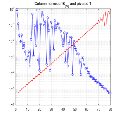
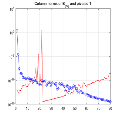
Fig. 1: The structure of the matrix $\mathbf{B}_{[22]}$ and its column pivoted triangular factor in line 6. during the first two iterations in Algorithm 1. In the first plot, showing the data in the first iteration, the column norms of $\mathbf{B}_{[22]}$ are marked with (red) $\cdot-$ and the column norms its triangular factor in the Businger-Golub pivoted QR factorization are marked with (blue) $\circ-$. The second plot shows the same information, but in the second iteration.

3.3 The Quandary of Column Scaling

In the VF literature, it is often recommended to scale the columns of the LS coefficient matrix in line 6 of Algorithm 1, to make them all of the same Euclidean length, before deploying the backslash solver, and then to rescale the solution, see, e.g., [34]. One desirable effect of this column equilibration step is to reduce the effective condition number of LS coefficient matrix (see e.g., [43, 55]). While this can be beneficial, nonetheless this tactic also may have a variety of deleterious effects and, in our opinion, must be considered with caution. Of foremost concern, following the discussion from §3.2, is that scaling noisy matrix columns effectively increases the influence of noise, and allows these noisy columns to participate in the column pivoting process of the QR factorization, with a possibility that some of them become drafted and taken upfront as important. This, in turn, interferes with the rank revealing process and possibly precludes truncation based on a partition as in (3.1). For illuminating discussions related to this issue we refer to [30], [29], [56]. In the following two examples we illustrate the potentially baleful effects of column scaling in the particular context of VF iteration.

Example 3.2.

We continue using the heat model from Example 3.1. In Figure 2 we show, for the first two iterations, the moduli of the diagonal entries ($|T_{ii}|$) of the triangular factors of $\mathbf{B}_{[22]}$ (appearing in line 6 of Algorithm 1) without and with column equilibration. Note that, due to the diagonal dominance (3.2), the distribution of $|T_{ii}|$ is decisive for numerical rank revealing.

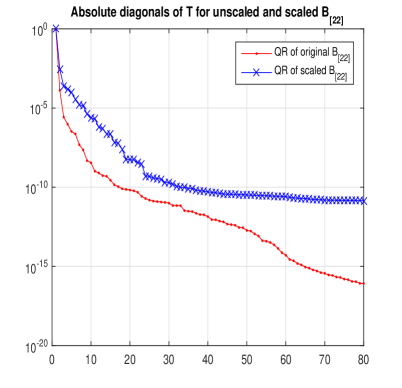
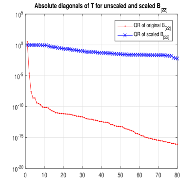
Fig. 2: (Example 3.1 cont.) The structure of the pivoted triangular factors (cf.(3.2)) of $\mathbf{B}_{[22]}$ in the first two iterations in Algorithm 1. The plot shows the values $|T_{ii}|$ of the unscaled $\mathbf{B}_{[22]}$ (marked with (red) $\cdot-$) and of the column equilibrated $\mathbf{B}_{[22]}$ (marked with (blue) $\times-$).

We now illustrate how the numerical rank deficiency may be manifested during the VF iterations. We solve the LS problems for the ${\boldsymbol{\varphi}}^{(k)}$s using only a simple modification of matlab’s backslash operator: first reorder the equations so that the rows of the coefficient matrix have decreasing $\ell_{\infty}$ norms, and then apply backslash. This stabilizes the LS solution process in much the same way as does Powell-Reid complete pivoting (see [15, 39]). We use $1000$ frequencies and $r=80$. The samples are matched perfectly with both our implementation of VF and vectfit3 [54] (up to relative errors of the order of $10^{-13}$). The first plot in Figure 3 shows the structure of the denominators ${\boldsymbol{\varphi}}^{(k)}$ throughout ten iterations. Each ${\boldsymbol{\varphi}}^{(k)}$ is represented by the sorted vector of $\log_{10}(|{\boldsymbol{\varphi}}^{(k)}|/\|{\boldsymbol{\varphi}}^{(k)}\|_{1})$, and the zero entries of ${\boldsymbol{\varphi}}^{(k)}$ are not shown. For $k=1,\ldots,10$, the values of $\textsf{sum}(|{\boldsymbol{\varphi}}^{(k)}|/\|{\boldsymbol{\varphi}}^{(k)}\|_{\infty}>\mbox{\boldmath$\varepsilon$})$ are, respectively, $53$, $43$, $38$, $30$, $44$, $44$, $44$, $40$, $42$, $44$. (If we restart the approximation with $r=53$, the number of nonzero coefficients throughout the iterations are $40$, $36$, $38$, $41$, $41$, $42$, $41$, $41$, $39$, $41$.) To interpret these numbers, we compute the Hankel singular values $\sigma_{1}\geq\cdots\geq\sigma_{197}$ and superimpose them on the graph as $\log_{10}(\sigma_{i}/\sigma_{1})$ – those values marked by $\diamond$. Since the $\sigma_{i}$s are forming a “devil’s staircase” and there is no clear cutoff index. For instance, $\sigma_{30}/\sigma_{1}\approx 1.28e-11$, $\sigma_{36}/\sigma_{1}\approx 2.17e-13$, $\sigma_{44}/\sigma_{1}\approx 1.12e-16$, $\sigma_{53}/\sigma_{1}\approx 9.00e-17$. (If we use the backslash without the initial row pivoting, the numbers of nonzero coefficients throughout the iterations are $53$, $44$, $37$, $42$, $50$, $50$, $50$, $49$, $49$, $50$.)

Recall from Proposition 1 that the barycentric nodes corresponding to $\varphi_{j}^{(k)}=0$ are the poles of the current approximant ${\mathbf{H}}_{r}^{(k)}$ and that the corresponding residues are accessible by an explicit formula (2.9), thus allowing an estimate of the contribution of the pole and perhaps discarding it and reducing $r$. The matching of the number of the untruncated entries in the LS solutions ${\boldsymbol{\varphi}}^{(k)}$ with the number of significant Hankel singular values is striking and may offer machinery to readjust the order of the approximant, $r$, during the iterations. This matching cannot be guaranteed in general but offers a great promise. Full understanding of the potential of the VF for determining the order of the underlying system (e.g., as in the Loewner framework [46]) remains an important open problem. The right-hand side plot in Figure 3 also shows $\log_{10}(|{\boldsymbol{\varphi}}^{(k)}|/\|{\boldsymbol{\varphi}}^{(k)}\|_{1})$, but with the column scaling of the least squares coefficient matrix and rescaling the solution, as in vectfit3. Note that, once the scaling is applied, connection to the Hankel singular values decay is lost; supporting our discussion on the undesirable effects of column scaling in VF.

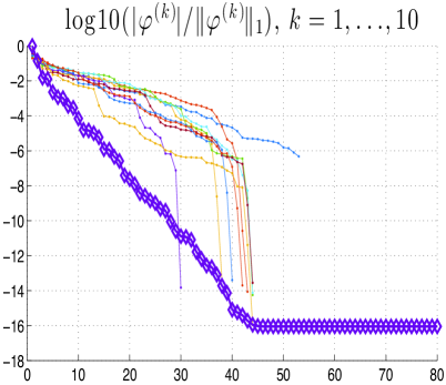
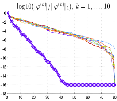
Fig. 3: (Example 3.2.) History of the first 10 iterations, $k=1,\ldots,10$. Plots show $log_{10}(|\varphi_{j}^{(k)}|//\|{\boldsymbol{\varphi}}^{(k)}\|_{1})$ vs $j$; only nonzero coefficients are shown. Normalized Hankel singular values are represented as diamonds.

3.4 mimoVF: Putting the pieces together

In this section, based on our preceding analysis of VF for matrix-valued rational approximation problem, we start testing our new implementation of VF. We will call the new implementation and the corresponding matlab toolbox mimoVF. This section will provide examples for verification and validation of mimoVF. We will compare our implementation with the original vectfit3 [54] and show that our proposed modifications based on the theoretical analysis can substantially improve the results. While on average vectfit3 performs well, in the ill-conditioned cases, it has difficulties with numerical issues addressed in this paper.

For the resulting rational approximation ${\mathbf{H}}_{r}$, define the tensor $\mathbb{S}_{r}(:,:,i)={\mathbf{H}}_{r}(\xi_{i})$, $i=1,\ldots,\ell$, and the relative LS error as ${\boldsymbol{\gamma}}=\|\mathbb{S}-\mathbb{S}_{r}\|_{F}/\|\mathbb{S}\|_{F}$. Recall that $\mathbb{S}(:,:,i)={\mathbf{H}}(\xi_{i})\in\mathbb{C}^{p\times m}$, $i=1,\ldots,\ell$, contains the original samples that are either measurements, or computed from a state space realization of the underlying LTI dynamical system.

3.4.1 A stress test

We consider a model for the ISS 1R module [13] with $m=p=3$. The underlying dynamical system has dimension $n=270$. This example presents a difficult test case with rather vivid dynamics. The model is very hard to approximate and presents significant challenges to model reduction; see [32]. To that end, we choose $r=50$ and take $\ell=300$ samples. The initial barycentric nodes are chosen as the eigenvalues of a pseudo-random real stable $r\times r$ matrix, a potentially poor initialization. Using these initial nodes, two iteration steps are taken both in vecfit3 and mimoVF. The goal of this example is to illustrate that once the computations in each iteration step are made more robust (following our preceding analysis), high-fidelity rational approximants can still be achieved even with a small number iteration count or even in the cases of poorly initial choices of barycentric nodes. The results of vectfit3 and mimoVF are shown on Figure 4 where we depict the amplitude frequency response plots for the data and for the rational approximants. Note that this model has $m=3$ inputs and $p=3$ outputs, there are $9$ input/output channels corresponding to the different lines in Figure 4. The figure clearly illustrates the mimoVF performs significantly better than vecfit3 for this example. Recall that both functions are given the same set of initial poles. Despite this unfavorable choice of initial poles, a restricted number of iterations, and ill-conditioned LS matrices, mimoVF succeeds to compute a model with relative LS error below $\gamma\approx 6.45\cdot 10^{-3}$. On the other hand, the relative error due to vectfit3 is $\gamma\approx 10.41$; a significantly higher value than the error due to mimoVF. It is possible that allowing vectfit3 to iterate further might realign the poles better, leading to a smaller LS error and an accurate approximate. But, of course, this comes with additional costs since every step of the iteration requires to solve a potentially large-scale LS problem; especially when $m$ and $p$ are large. Therefore, any reduction in the iteration count is a gain in terms of computational efficiency.

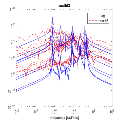
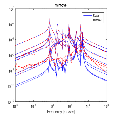
Fig. 4: (Example of §3.4.1.) Comparison of mimoVF and the vectfit3 on the ISS 1R module with initial poles set as the eigenvalues of a pseudo-random stable real matrix, $\ell=300$ and $r=50$. (The frequency response magnitudes of each of the possible nine input/output pairings is plotted in solid blue; the corresponding frequency response magnitudes from rational approximations provided by vectfit3 and mimoVF appear as dashed red lines.) The purpose of the experiment is to check the robustness of the numerical implementation in the case of unpropitious distribution of the barycentric nodes. The first plot shows the output of vectfit3 (with the relative error $\gamma>10$), and the second of mimoVF ($\gamma<10^{-2}$), both after two iterations.

3.4.2 How to compute the residues in the final step

One of the advantages of the barycentric implementation of the SK iterations over the original approach using polynomial representations is in the avoidance of high powers of $\xi_{i}$ (which may cause overflow and underflow in finite precision arithmetic) as producing ill-conditioned Vandermonde matrices. The additional scalings by $1/|d^{(k)}(\xi_{i})|^{2}$, which is another potential source of ill-conditioning, has been elegantly removed by the VF formulation and compensated by reallocating the barycentric nodes $\lambda_{j}^{(k)}$. However, once the VF iterations are completed, one needs to solve for the final residues ${\boldsymbol{\Phi}}$ in Line 9. of Algorithm 1 for the converged poles. This step needs to be performed carefully as the coefficient matrix that determines the residues for given set of poles is a Cauchy matrix, which, together with Vandermonde matrices, is among the most notoriously ill-conditioned matrices. To illustrate, the spectral condition number of an arbitrary $100\times 100$ real Vandermomde matrix is larger than $3\cdot 10^{28}$, and the condition number of the $100\times 100$ Hilbert (Cauchy) matrix is more than $10^{150}$. The column norms of the latter are between $0.07$ and $1.3$, thus no column scaling can substantially reduce the condition number. Furthermore, the additional weightings $\rho_{i}$ (whose values may spread many orders of magnitude) may further worsen the conditioning of the least squares coefficient matrix. This all is a menace to the final computed residues, in particular when the order $r$ is sufficiently high and in cases of unfavorably distributed nodes. This issue has to be addressed if the method is to be applied to truly challenging problems with complex dynamics and of high orders, for instance, for $m,p,r$ in hundreds. In this section we focus our attention to the very last step – given poles of a rational approximant, how to best numerically extract the residues.

Example 3.3.

We continue to use the ISS 1R example from §3.4.1. However, in this case, we choose good initial poles of the form $\lambda_{j}=\alpha_{j}\pm{\dot{\imath\mskip-3.0mu\imath}}\beta_{j}$, where the (positive) $\beta_{j}$s are log-spaced over the frequency sample interval and $\alpha_{j}=-\beta_{j}$ as often recommended in the VF literature for good initial pole selection. We take $\ell=500$ and choose $r=100$. Recall that the underlying system has dimension $n=270$ with $p=m=3$; therefore with $r=100$ and $\ell=500$ samples, one expects to obtain a very good approximation. The amplitude frequency response plots are depicted in Figure 5 for both vecfit3 and mimoVF, once again illustrating that mimoVF outperforms vecfit3; the relative LS errors due to mimoVF and vecfit3 are respectively, $9.47\cdot 10^{-1}$ and $4.90\cdot 10^{-3}$. In this case, vecfit3 suffers from the numerical ill-conditioning of the final residue computation. Thus, this example shows that even a plenty of good initial barycentric nodes, one does not necessarily guarantee a good approximation due to the numerical issues arising in the residue computation step.

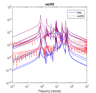
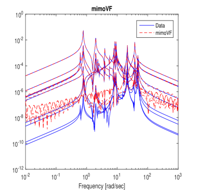
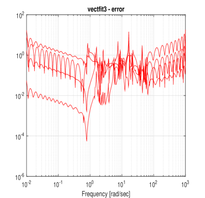
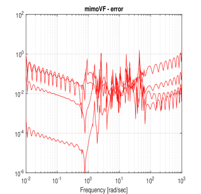
Fig. 5: (Example 3.3.) Comparison of mimoVF and the vectfit3 on an ISS example with initial poles set as log-spaced (imaginary parts log-spaced over the frequency range). The first plot shows the output of vectfit3 (with the relative error $\gamma\approx 9.47\cdot 10^{-1}$), and the second of mimoVF ($\gamma\approx 4.90\cdot 10^{-3}$) after one iteration. In this example, $\ell=500$ and $r=100$. The second row shows relative approximation error $|{\mathbf{H}}(\xi_{i})_{uv}-{\mathbf{H}}_{r}(\xi)_{uv}|/|{\mathbf{H}}(\xi_{i})_{uv}|$ for the four dominant input-output pairs over all samples. Since the order of the underlying system is $n=270$ and $p=m=3$, $r=100$ should provide good approximation.

A regularization approach for residue extraction

Even though mimoVF performed relatively well in Example 3.3, some of the less-dominant input/output pairs were not captured as accurately as one would prefer; see Figure 5. In this section, we consider a regularization technique to further improve the final residue extraction step in mimoVF. Recall Line 9. of Algorithm 1 to compute the final residues: solving ${\boldsymbol{\Phi}}={\mathbf{B}}_{[11]}^{-1}\mathbf{s}_{1}$. As noted in Remark 2.1 this corresponds to the simultaneous determination of the residue matrices by solving $\|{\mathcal{D}}_{\rho}\left({\mathscr{C}}^{(k+1)}\varPhi^{(k+1)}(u,v,:)-\mathbb{S}(u,v,:)\right)\|_{2}\longrightarrow\min$, $u=1,\ldots,p$, $v=1,\ldots,m$. To simplify the notation, denote this LS problem by $\|{\mathcal{D}}_{\rho}{\mathscr{C}}x-h\|_{2}\longrightarrow\min$, where ${\mathscr{C}}={\mathscr{C}}_{{\boldsymbol{\xi}},{\boldsymbol{\lambda}}}$ is a Cauchy matrix as in (2.11), $h$ is the corresponding scaled right-hand side, ${\boldsymbol{\lambda}}$ is closed under conjugation and and the solution vector should also be closed under conjugation. Such a constrained problem can be replaced by an equivalent unconstrained LS problem

$$\left\|\begin{pmatrix}{\mathcal{D}}_{\rho}{\mathscr{C}}_{{\boldsymbol{\xi}},{\boldsymbol{\lambda}}}\cr{\mathcal{D}}_{\rho}{\mathscr{C}}_{\overline{{\boldsymbol{\xi}}},{\boldsymbol{\lambda}}}\end{pmatrix}x-\begin{pmatrix}h\cr\overline{h}\end{pmatrix}\right\|_{2}\equiv\|\widehat{{\mathscr{C}}}x-\widehat{h}\|_{2}\longrightarrow\min$$ (3.6)

with the coefficient matrix again of the diagonally scaled Cauchy structure, $\widehat{{\mathscr{C}}}=({\mathcal{D}}_{\rho}\oplus{\mathcal{D}}_{\rho}){\mathscr{C}}_{({\boldsymbol{\xi}},\overline{{\boldsymbol{\xi}}}),\lambda}$.

The SVD of $\widehat{{\mathscr{C}}}$ can be computed to high relative accuracy based on the pivoted LU decomposition $\Pi_{1}\widehat{{\mathscr{C}}}\Pi_{2}=LDU$, where each entry (including the tiniest ones) of the computed factors $\widetilde{L}$, $\widetilde{D}$, $\widetilde{U}$ is computed to high relative accuracy, and $\widetilde{L}$, $\widetilde{U}$ are well conditioned. The ill-conditioning of $\widehat{{\mathscr{C}}}$ is revealed in the diagonal matrix $\widetilde{D}$. This decomposition can be used immediately in an LS solver [12], or it can be used to compute an accurate SVD [18], [16], [27, 28] which is then used to compute an approximate LS solution. $\widehat{{\mathscr{C}}}$ can be severely ill-conditioned so that small changes of $\xi_{i}$s and $\lambda_{j}$s can cause significant perturbation of the SVD. However, we can consider the values of $\xi_{i}$s and $\lambda_{j}$s, as stored in the machine memory, as exact and attempting to compute accurate SVD is justified.

Let $\widehat{{\mathscr{C}}}=W\Sigma V^{*}$ be the SVD and let the unique LS solution be $x=V\Sigma^{\dagger}W^{*}=\sum_{i=1}^{r}v_{i}(w_{i}^{*}\widehat{h})/\sigma_{i}$. Unfortunately, an accurate SVD is not enough to have the LS solution computed to high relative accuracy, and additional regularization techniques must be deployed. This is in particular important if the right-hand side is contaminated by noise. In the Tichonov regularization, we choose $\mu\geq 0$ and use the solution of $\|\widehat{{\mathscr{C}}}x-\widehat{h}\|_{2}^{2}+\mu^{2}\|x\|_{2}^{2}\rightarrow\min$, explicitly computable as

$$x_{\mu}=\sum_{i=1}^{r}\frac{\sigma_{i}}{\sigma_{i}^{2}+\mu^{2}}(w_{i}^{*}\widehat{h})v_{i}.$$ (3.7)

The parameter $\mu$ can be further adjusted using the Morozov discrepancy principle [48], i.e., to achieve $\|\widehat{{\mathscr{C}}}x_{\mu}-\widehat{h}\|_{2}\approx\nu$, where $\nu$ is the estimated level of noise $\delta\widehat{h}$ in the right-hand side, $\nu\approx\|\delta\widehat{h}\|_{2}$.

Example 3.4.

Here we continue Example 3.3, use the same data, and apply vecfit3 and mimoVF where we use the preceding regularization approach in the final residue computation step. Using accurate SVD of $\widehat{{\mathscr{C}}}$ we compute $x_{\mu}$ as in (3.7) with an ad hoc choice of $\mu=10^{-3}$. The results after only one iteration of mimoVF and two iterations of vectfit3 are shown on Figure 6. mimoVF still has smaller LS error; $4.90\cdot 10^{-3}$ compared to $1.77\cdot 10^{-1}$ due to vectfit3. It is important to note that mimoVF achieves this better performance after only one iteration. vectfit3 has the error of $1.77\cdot 10^{-1}$ after two iterations. This shows that a more robust implementation may reduce the total number of iterations needed to reach satisfactory approximation; thus reducing the overall computational complexity.

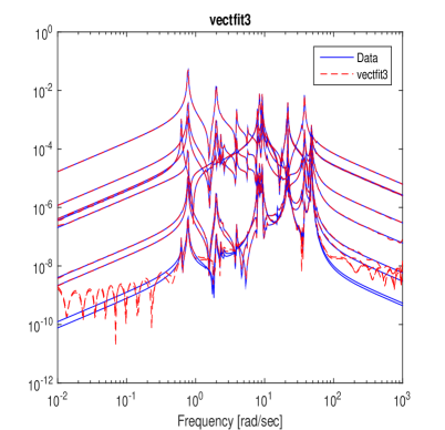
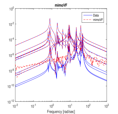
Fig. 6: Comparison of mimoVF and the vectfit3 on an ISS example with initial poles set as log-spaced (imaginary parts log-spaced over the frequency range). In this example, $\ell=500$ and $r=100$. The first plot shows the output of vectfit3 after two iterations (with the relative error $\gamma\approx 1.77\cdot 10^{-1}$), and the second of mimoVF ($\gamma\approx 4.90\cdot 10^{-3}$) after one iteration.

Remark 3.1.

The LDU decomposition, which is the initial step of the accurate SVD, can also be used in the pole identification phase to compute accurate QR factorization of Cauchy matrices at all stages of the computation. We have not included those modifications, for the sake of brevity of the presentation. Interested readers can find the details of such an approach in [24].

3.4.3 Stopping criterion

It should be noted that the stopping criterion in the VF framework is rather vaguely specified. To the best of our knowledge, the VF literature does not provide a precise and numerically justified strategy of halting the iterations. For instance, vectfit3 allows only running for a given fixed number of iterations.

Following our recent analysis [26], we propose to declare the $|{\varphi}_{j}^{(k+1)}|$s “small enough” if

$$\sum_{j=1}^{r}\frac{|{\varphi}_{j}^{(k+1)}|}{|\Re{e}(\lambda_{j}^{(k+1)})|}\equiv\theta^{(k+1)}\leq{\boldsymbol{\epsilon}},\;\;\mbox{where ${\boldsymbol{\epsilon}}$ is a suitable threshold.}$$ (3.8)

This seems appropriate because $\max_{s\in{\dot{\imath\mskip-3.0mu\imath}}\mathbb{R}}|d^{(k+1)}(s)-1|\leq\theta^{(k+1)}$, and in (2.6) we can write

$${\mathbf{S}}^{(i)}(1+\sum_{j=1}^{r}\frac{{\varphi}_{j}^{(k+1)}}{\xi_{i}-\lambda_{j}^{(k+1)}})={\mathbf{S}}^{(i)}+\Delta{\mathbf{S}}^{(i)},\;\;\|\Delta{\mathbf{S}}^{(i)}\|_{F}\leq\theta^{(k+1)}\|{\mathbf{S}}^{(i)}\|_{F},$$

thus interpreting this as introducing backward perturbation into the data. In fact, this interpretation can be a guidance for choosing the threshold value ${\boldsymbol{\epsilon}}$ by following a discrepancy principle, i.e., so that this backward error matches the estimated size of the noise level on the input.

3.5 Guidelines for efficient implementation

We now further discuss implementation details that are relevant for an efficient software implementation of mimoVF or Algorithm 1 in general. Recall that VF for MIMO systems with $m$ input and $p$ inputs will require $p\cdot m$ QR factorizations (2.12) of size $\ell\times(2r)$ before advancing toward finding $\varphi_{j}^{(k+1)}$. It is clear that this is a demanding computational challenge even for moderate $m$ and $p$; e.g., in the case $m=p=100$, it will require $p\cdot m=10000$ QR factorizations of size $\ell\times(2r)$. Since these factorizations are independent, they can be very efficiently parallelized and the whole computation can be optimized for a multi-core computing machinery. This has been nicely described by Chinea and Grivet-Talocia [14], who showed a nearly ideal speedup on a four quad-core architecture.

3.5.1 Efficient computation of $\mathbf{B}_{[22]}$

It was pointed out earlier that the QR factorizations in (2.12) are independent of $(u,v)$ in the first $r$ columns and $(R^{(k+1)})_{11}$ from (2.15) can be computed by a single QR factorization, optionally with column pivoting, of ${\mathcal{D}}_{\rho}{\mathscr{C}}^{(k+1)}$, i.e., ${\mathcal{D}}_{\rho}{\mathscr{C}}^{(k+1)}\Pi=V^{(k+1)}\left(\begin{smallmatrix}T^{(k+1)}\cr 0\end{smallmatrix}\right)$. Further, the introduction of rank-revealing column pivoting $\Pi$ in this factorization incurs a negligible overhead, while preserving the structure (2.16). We discussed in §3.1 that this pivoting is very important for numerical robustness of the LS solution as well. In an LAPACK-style implementation, the matrix $V^{(k+1)}$ can be computed and stored in form of $r$ Householder vectors (using Xgeqp3), and then, using Xormqr, $(V^{(k+1)})^{*}$ can be concurrently applied to all $-{\mathcal{D}}_{\rho}D^{(uv)}{\mathscr{C}}^{(k+1)}$, $u=1,\ldots,p$, $v=1,\ldots,m$. Then, it only remains to compute the QR factorizations of the $(r+1:\ell,r+1:2r)$ submatrices of $-(V^{(k+1)})^{*}{\mathcal{D}}_{\rho}D^{(uv)}{\mathscr{C}}^{(k+1)}$. One should note that in a blocked QR factorization a similar computation is done anyway in the process of computing the QR factorizations (2.12). The computed triangular $r\times r$ factors are the $(2,2)$ blocks in (2.12) that build the matrix $\mathbf{B}_{[22]}^{(k+1)}$. Hence, the saving of this modified approach is equivalent to the cost of $(pm-1)$ QR factorizations of size $\ell\times r$, or, approximately, $const\cdot(pm-1)\ell r^{2}$. The total work on the QR factorizations (2.12) without this modification is $4\cdot const\cdot pm\ell r^{2}$.

Further, when we are solving only for the $\varphi_{j}^{(k)}$ during the VF iterations, the elements of $\mathcal{Q}^{*}A$, denoted by $\times$ in (2.12) and (2.16) are not used in the pole identification phase, but they are computed as $(R^{(k+1)}_{uv})_{12}$ parts of the QR factorizations (2.12). On the other hand, once the poles are fixed, the LS problem is solved with the approximant of the form (2.2), but with the unit denominator, $d^{(k)}(s)\equiv 1$, or, equivalently, with $\varphi_{j}^{(k+1)}=0$, $j=1,\ldots,r$. This means that, for computing (2.7) by the Algorithm 1, we do not compute the matrices $(R^{(k+1)}_{uv})_{12}$, which further reduces the complexity. Our implementation of this more efficient approach is based on adapting the LAPACK’s functions Xormqr, Xlarft and Xlarfb.

3.5.2 Locally pivoted factorization

In the presence of noise and ill-conditioning, pivoting is essential when using the QR factorization. Hence, we propose to include pivoting in the procedure outlined in §3.5.1. More precisely, the QR factorization of ${\mathcal{D}}_{\rho}{\mathscr{C}}^{(k+1)}$ is computed with column pivoting, i.e., ${\mathcal{D}}_{\rho}{\mathscr{C}}^{(k+1)}\Pi^{(k+1)}=V^{(k+1)}\left(\begin{smallmatrix}T^{(k+1)}\cr 0\end{smallmatrix}\right)$. This enhances the accuracy of the computed residues in line 9. of Algorithm 1. In a software implementation, Line 9. is reshaped into the LS problem with the coefficient matrix $T^{(k+1)}$ and with $m\cdot p$ right-hand sides, for all input-output pairs. Optionally, one can use the truncation discussed in §3.1, or the accurate SVD as explained in §3.4.2.

Further, we also advocate the use of pivoting when computing the QR factorizations of the $(r+1:\ell,r+1:2r)$ submatrices of $-(V^{(k+1)})^{*}{\mathcal{D}}_{\rho}D^{(uv)}{\mathscr{C}}^{(k+1)}$. This increases the accuracy of the computed matrix $\mathbf{B}_{[22]}^{(k+1)}$ in line 6. For details how pivoting influences the accuracy of the rows of the computed triangular QR factor we refer to [25]. Furthermore, this may allow (in the cases of numerical rank deficiency, as revealed by the pivoted QR factorization and discussed in §3.1) to set certain numbers of rows of $(R^{(k+1)}_{uv})_{22}$ to zero and thus increased the number of zero rows in $\mathbf{B}_{[22]}^{(k+1)}$ and reduced the complexity of Line 6 in Algorithm 1, where, as described in §3.1, the LS solver starts with the QR factorization with column pivoting.

The pivoted QR factorization of the tall and skinny matrix $\mathbf{B}_{[22]}^{(k+1)}$ can be computed by e.g., first computing the QR without pivoting using the techniques of [9], and then computing the pivoted QR factorization of the computed $r\times r$ triangular factor, or e.g. as in [17]. These approaches become particularly attractive if $p\cdot m$ and $r$ are large.

Remark 3.2.

Interestingly, we do not need to compute the $(R^{(k+1)}_{uv})_{22}$s. Instead, we can build the matrix $\mathbf{B}_{[22]}^{(k+1)}$ from the $(r+1:\ell,r+1:2r)$ submatrices of $-(V^{(k+1)})^{*}{\mathcal{D}}_{\rho}D^{(uv)}{\mathscr{C}}^{(k+1)}$. This will lead to increased number of rows in $\mathbf{B}_{[22]}^{(k+1)}$, but overall it reduces the complexity with potential gain increased if the QR factorization of $\mathbf{B}_{[22]}^{(k+1)}$ is computed using the strategies of [9], [17].

4 Numerical Quadrature in mimoVF for discretized $\mathcal{H}_{2}$ approximation

The framework for mimoVF is based on the algebraic least squares (LS) error minimization (1.1) where one usually chooses the weights $\rho_{j}=1$ and the nodes $\xi_{j}$ are usually selected heuristically. In [26], for single-input/single-output (SISO) systems, we have shown that with the underlying dynamical system in mind, reformulating the discrete LS problem as discretization of an underlying continuos $\mathcal{H}_{2}$ error measure and then choosing the nodes and weights by an appropriate numerical quadrature improves the performance of VF significantly. The same conclusion holds in the MIMO case as well since, once the common set of poles has been determined, mimoVF works separately on each input–to-output pair. We illustrate these considerations briefly in this section.

4.1 $\mathcal{H}_{2}$ approximation and numerical quadrature

The algebraic least squares error is closely related to the $\mathcal{H}_{2}$ system norm. More precisely, consider the space $\mathcal{H}_{2,+}^{p\times m}$ of $p\times m$ matrix functions ${\mathbf{M}}(s)$, analytic in the open right half-plane $\mathbb{C}_{+}=\{s\in\mathbb{C}\;:\;\Im(s)>0\}$, such that $\sup_{x>0}\int_{\infty}^{\infty}\|{\mathbf{M}}(x+{\dot{\imath\mskip-3.0mu\imath}}y)\|_{F}^{2}dy<\infty$. The space $\mathcal{H}_{2,+}^{p\times m}$is a Hilbert space with the associated inner product and norm defined by

$$\langle{\mathbf{M}}_{1},{\mathbf{M}}_{2}\rangle_{\mathcal{H}_{2}}=\frac{1}{2\pi}\int_{-\infty}^{\infty}\mathrm{Trace}\left(\overline{{\mathbf{M}}_{1}({\dot{\imath\mskip-3.0mu\imath}}\omega)}{\mathbf{M}}_{2}({\dot{\imath\mskip-3.0mu\imath}}\omega)^{T}\right)\,d\omega,\;\;\;\|{\mathbf{M}}\|_{\mathcal{H}_{2}}=\left(\frac{1}{2\pi}\int_{-\infty}^{\infty}\left\|{\mathbf{M}}({\dot{\imath\mskip-3.0mu\imath}}\omega)\right\|_{F}^{2}\,d\omega\right)^{1/2}.$$ (4.1)

The $\mathcal{H}_{2}$ approximation problem is, then, to find a degree-$r$ rational approximant, ${\mathbf{H}}_{r}(s)$, that minimizes the $\mathcal{H}_{2}$ error norm $\|{\mathbf{H}}-\widetilde{{\mathbf{H}}}_{r}\|_{\mathcal{H}_{2}}$ over all degree-$r$ rational function $\widetilde{{\mathbf{H}}}_{r}(s)$. Such an optimal rational approximant must satisfy certain Hermite tangential interpolation conditions; for details we refer to [5, 33]. The Iterative Rational Krylov Algorithm (IRKA) of Gugercin et al. [33] is a numerically effective iterative algorithm that constructs degree-$r$ rational approximatants satisfying the $\mathcal{H}_{2}$-optimality conditions.

Our goal in this section is to repeat the success of [26] for SISO systems, i.e., improve the performance of mimoVF by formulating the discrete LS measure as discretization of the continuous $\mathcal{H}_{2}$ error. Towards this goal, approximate the $\mathcal{H}_{2}$ error with a quadrature role to obtain

$$\int_{-\infty}^{+\infty}\mskip-3.0mu\mskip-3.0mu\mskip-3.0mu\|{\mathbf{H}}({\dot{\imath\mskip-3.0mu\imath}}\omega)-{\mathbf{H}}_{r}({\dot{\imath\mskip-3.0mu\imath}}\omega)\|_{F}^{2}d\omega \approx \sum_{j=1}^{\ell}\rho_{j}^{2}\|{\mathbf{H}}(\xi_{j})-{\mathbf{H}}_{r}(\xi_{j})\|_{F}^{2}+\rho_{+}^{2}\,M_{+}[|{\mathbf{H}}-{\mathbf{H}}_{r}|^{2}]+\rho_{-}^{2}\,M_{-}[|{\mathbf{H}}-{\mathbf{H}}_{r}|^{2}]~{}~{}~{}~{}$$ (4.2)

where $M_{\pm}[G]$ are linear functionals of $G$ that capture information about asymptotic behavior of $G$ at $\pm\infty$. Note that the usual VF formulation correspond to $\rho_{+}=\rho_{-}=0$, with all other $\rho_{j}=1$, and choosing sampling nodes $\xi_{j}$ to be equidistant and in complex conjugate pairs. Thus, the usual VF objective function is as a composite trapezoid quadrature rule for the integral in (4.2) approximating the $\mathcal{H}_{2}$ error. As we discussed in [26], more effective quadrature options may be considered, e.g., Gauss-Legendre, Gauss-Kronrod, and Gauss-Hermite quadrature rules. We do not go into the details of what quadrature method to choose here; since our main point is just to illustrate that mimoVF can perform much better once formulated as a discretized $\mathcal{H}_{2}$ measure.

4.2 A numerical example

Here, with a simple example, we illustrate the effect of choosing the sampling points and the weights using numerical quadrature. We use the Clenshaw-Curtis type quadrature rule developed by Boyd [10]. We use the ISS 1R module [32] with $m=3$ inputs and $p=3$ outputs. We use only $100$ function evaluations ($\ell=200$) and apply mimoVF to this data set for different $r$ values. Resulting relative $\mathcal{H}_{2}$ errors are shown in Table 1 below. The quadrature-based selection yields the smallest error in each case; for $r=20$ and $r=30$, it leads to one order of magnitude improvements.

Method	$r=10$	$r=20$	$r=30$	$r=40$
mimoVF without Quadrature	$3.4104\times 10^{-1}$	$3.1775\times 10^{-1}$	$1.2778\times 10^{-1}$	$5.0257\times 10^{-2}$
mimoVF without Quadrature	$2.5209\times 10^{-1}$	$4.6074\times 10^{-2}$	$3.3226\times 10^{-2}$	$2.1436\times 10^{-2}$

Table 1: Effect of quadrature nodes and weights on mimoVF

5 Controlling the McMillan Degree

Let $\{{\boldsymbol{\Phi}}_{j}\}_{1}^{r}\subset{\mathbb{C}}^{p\times m}$ and $\{\lambda_{j}\}_{1}^{r}\subset{\mathbb{C}}$ denote the final set of matrix residues and poles, respectively, resulting from mimoVF. To ease notational clutter, we drop the iteration index $k$. The associated rational matrix approximant can be represented as

$${\mathbf{H}}_{r}(s)=\sum_{j=1}^{r}\frac{{\boldsymbol{\Phi}}_{j}}{s-\lambda_{j}}=\left(\begin{smallmatrix}\mathbb{I}_{p}&\ldots&\mathbb{I}_{p}\end{smallmatrix}\right)\mskip-3.0mu\mskip-3.0mu\left(\begin{smallmatrix}\frac{\mathbb{I}_{p}}{s-\lambda_{1}}&&\cr&\ddots&\cr&&\frac{\mathbb{I}_{p}}{s-\lambda_{r}}\end{smallmatrix}\right)\mskip-3.0mu\mskip-3.0mu\left(\begin{smallmatrix}{\boldsymbol{\Phi}}_{1}\cr\vdots\cr{\boldsymbol{\Phi}}_{r}\end{smallmatrix}\right)=\left(\begin{smallmatrix}{\boldsymbol{\Phi}}_{1}&\ldots&{\boldsymbol{\Phi}}_{r}\end{smallmatrix}\right)\mskip-3.0mu\mskip-3.0mu\left(\begin{smallmatrix}\frac{\mathbb{I}_{m}}{s-\lambda_{1}}&&\cr&\ddots&\cr&&\frac{\mathbb{I}_{m}}{s-\lambda_{r}}\end{smallmatrix}\right)\mskip-3.0mu\mskip-3.0mu\left(\begin{smallmatrix}\mathbb{I}_{m}\cr\vdots\cr\mathbb{I}_{m}\end{smallmatrix}\right)$$ (5.1)

If ${\mathbf{H}}_{r}(s)$ has simple poles, then ${\mathbf{H}}_{r}(s)$ has nominal McMillan degree $\mathsf{deg}({\mathbf{H}}_{r}(s))=\sum_{j=1}^{r}\mathsf{rank}({\boldsymbol{\Phi}}_{j})$. Evidently, $r\leq\mathsf{deg}({\mathbf{H}}_{r}(s))\leq r\min(p,m)$. Note that $\mathsf{deg}({\mathbf{H}}_{r}(s))$ will be strictly larger than $r$ unless the residues, ${\boldsymbol{\Phi}}_{j}$, all have rank $1$, and indeed, $\mathsf{deg}({\mathbf{H}}_{r}(s))$ can be potentially much larger than $r$ if either the input space or output space has significant dimension. McMillan degree is a proxy for the complexity involved in evaluating an approximant, therefore it is generally desirable and sometimes necessary to reduce the McMillan degree of a rational approximant to the target value of $r$, while retaining its approximating quality as much as possible. One straightforward method to accomplish this is to use truncation as suggested in [37]: For each $j=1,\,\ldots,\,r$, find the best rank-one approximation of ${\boldsymbol{\Phi}}_{j}\approx\ c_{j}\,b_{j}^{T}$ where $c_{j}\in{\mathbb{C}}^{p}$ and $b_{j}\in{\mathbb{C}}^{m}$. However, it is often the case that the residues ${\boldsymbol{\Phi}}_{j}$ are not close to rank–one matrices and so, truncation to rank-one residues can substantially increase the LS error. [37] suggested using the SVD to determine the numerical ranks of the ${\boldsymbol{\Phi}}_{j}$s and truncating them to their respective best low-rank (not necessarily rank–one) approximations; [37] also proposed Gauss-Newton correction, but no details on how to proceed in this direction were provided.

We propose here two different approaches toward retaining rank-$1$ residues, allowing us to achieve a true McMillan degree of $r$ while keeping the approximation quality as high as possible. The first approach, presented in §5.1, is based on a nonlinear least-squares minimization, the second one, presented in §5.2, combines mimoVF with well-established optimal systems-theoretic model reduction methodologies.

5.1 Rank-one residue correction via Alternating Least Squares

We seek an optimal rational approximant, $\widehat{{\mathbf{H}}}_{r}(s)$, having the same poles, $\{\lambda_{j}\}_{1}^{r}$, as the mimoVF approximant, but taking the form

$$\widehat{{\mathbf{H}}}_{r}(s)=\sum_{j=1}^{r}\frac{c_{j}b_{j}^{T}}{s-\lambda_{j}}\equiv C(s\mathbb{I}-\Lambda)^{-1}B^{T},\;\;\mbox{where}\;\;\Lambda=\mathrm{diag}(\lambda_{j})_{j=1}^{r},\;\;\begin{array}[]{l}C=\begin{pmatrix}c_{1}&\ldots&c_{r}\end{pmatrix}\cr B=\begin{pmatrix}b_{1}&\ldots&b_{r}\end{pmatrix}.\end{array}$$ (5.2)

Optimality here will mean that $C$ and $B$ are chosen so that $\widehat{{\mathbf{H}}}_{r}(s)$ satisfies

$$\min_{C,\ B}\sum_{i=1}^{\ell}\|\sum_{j=1}^{r}\frac{c_{j}b_{j}^{T}}{\xi_{i}-\lambda_{j}}-{\mathbf{H}}(\xi_{i})\|_{F}^{2}=\min_{C,\ B}\|\underbrace{({\mathscr{C}}\otimes\mathbb{I}_{p})}_{\mathcal{M}}\begin{pmatrix}c_{1}b_{1}^{T}\cr\vdots\cr c_{r}b_{r}^{T}\end{pmatrix}-\begin{pmatrix}{\mathbf{H}}(\xi_{1})\cr\vdots\cr{\mathbf{H}}(\xi_{\ell})\end{pmatrix}\|_{F}^{2}.$$ (5.3)

A weighting factor $\rho_{i}>0$ can also be attached to each sample; yet for simplicity of presentation, we take all $\rho_{i}=1$. In (5.3), ${\mathscr{C}}\in\mathbb{C}^{\ell\times r}$ denotes the Cauchy matrix ${\mathscr{C}}_{ij}=1/(\xi_{i}-\lambda_{j})$. In many applications, $\widehat{{\mathbf{H}}}_{r}(s)$ should be real-valued for real-valued $s$. In that case, a constraint is added that the poles $\lambda_{j}$ and the residues $c_{j}b_{j}^{T}$ must be closed under conjugation: all non-real poles appear in complex conjugate pairs, say $\lambda_{j},\lambda_{j+1}=\overline{\lambda_{j}}$; $c_{j}$, $b_{j}$ are real if $\lambda_{j}$ is real, otherwise $c_{j+1}=\overline{c_{j}}$, $b_{j+1}=\overline{b_{j}}$.

The nonlinearity of the LS error (5.3) with respect to the variables, $B$ and $C$, can be evaded by reformulating the problem in terms of alternating least squares (ALS): if $B$ (alternatively, $C$) is fixed, then (5.3) becomes a linear least squares problem in terms of $C$ (alternatively, $B$). So, we minimize alternately with respect to $C$ (holding $B$ fixed) and then with respect to $B$ (holding $C$ fixed), repeating the cycle until convergence. We provide some algorithmic details below and illustrate the effectiveness of ALS iteration with an example. An analogous approach has been used for “residue correction” in realization-independent (data-driven) approaches to optimal $\mathcal{H}_{2}$ model reduction [7].

Correction of $C$

Assume $B$ is fixed and seek an updated $C$ (with conforming conjugation symmetry) that will minimize the LS error (5.3). To that end, we vectorize the error matrix column-wise and write the $k$th column ($k=1,\ldots,m$) of the residual matrix in (5.3) as

$$\mathcal{M}\begin{pmatrix}(b_{1})_{k}\mathbb{I}&&\cr&\ddots&\cr&&(b_{r})_{k}\mathbb{I}\end{pmatrix}\begin{pmatrix}c_{1}\cr\vdots\cr c_{r}\end{pmatrix}-\begin{pmatrix}{\mathbf{H}}(\xi_{1})e_{k}\cr\vdots\cr{\mathbf{H}}(\xi_{\ell})e_{k}\end{pmatrix}=\mathcal{M}(\mathrm{diag}(B(k,:))\otimes\mathbb{I}_{p})\begin{pmatrix}c_{1}\cr\vdots\cr c_{r}\end{pmatrix}-\begin{pmatrix}{\mathbf{H}}(\xi_{1})e_{k}\cr\vdots\cr{\mathbf{H}}(\xi_{\ell})e_{k}\end{pmatrix}.$$ (5.4)

Stacking all columns together, the problem becomes: minimize the Euclidean norm of the residual

$$\begin{pmatrix}\mathcal{M}(\Delta_{1}\otimes\mathbb{I}_{p})\cr\hline\cr\vdots\cr\hline\cr\mathcal{M}(\Delta_{m}\otimes\mathbb{I}_{p})\end{pmatrix}\begin{pmatrix}c_{1}\cr\vdots\cr c_{r}\end{pmatrix}-\begin{pmatrix}{\mathbf{H}}(\xi_{1})e_{1}\cr\vdots\cr{\mathbf{H}}(\xi_{\ell})e_{1}\cr\hline\cr\vdots\cr\hline\cr{\mathbf{H}}(\xi_{1})e_{m}\cr\vdots\cr{\mathbf{H}}(\xi_{\ell})e_{m}\end{pmatrix},\;\;\mbox{where}\;\;\Delta_{i}=\mathrm{diag}(B(i,:)),\;\;i=1,\ldots,m,$$ (5.5)

with conjugation symmetry constraints: $c_{j}$ is real if $\lambda_{j}$ is real and $c_{k}=\overline{c_{j}}$, if $\lambda_{k}=\overline{\lambda_{j}}$. Note that the number of rows above is $\ell\cdot m\cdot p$, and the number of unknowns is $p\cdot r$. In practice, $\ell$ is much larger than $m,p,r$, and it is always assumed that $\ell\geq 2r$.

Let ${\mathscr{C}}=Q\left(\begin{smallmatrix}R\cr 0\end{smallmatrix}\right)=\widehat{Q}R$ be the QR factorization, where $Q=\begin{pmatrix}\widehat{Q}&\breve{Q}\end{pmatrix}$, $\widehat{Q}=Q(:,1:r)$. Then $\mathcal{M}=(Q\otimes\mathbb{I}_{p})(\left(\begin{smallmatrix}R\cr 0\end{smallmatrix}\right)\otimes\mathbb{I}_{p})$ is the QR factorization of $\mathcal{M}$. Multiplying the blocks in the residual (5.5) by $(Q^{*}\otimes\mathbb{I}_{p})$ and using the block-partitioned structure of $Q$, we obtain an equivalent LS problem:

$$\left\|\begin{pmatrix}(R\otimes\mathbb{I}_{p})(\Delta_{1}\otimes\mathbb{I}_{p})\cr 0\cr\hline\cr\vdots\cr\hline\cr(R\otimes\mathbb{I}_{p})(\Delta_{m}\otimes\mathbb{I}_{p})\cr 0\end{pmatrix}\begin{pmatrix}c_{1}\cr\vdots\cr c_{r}\end{pmatrix}-\begin{pmatrix}(\widehat{Q}^{*}\otimes\mathbb{I}_{p})\mathrm{vec}(\mathbb{S}(:,1,:))\cr(\breve{Q}^{*}\otimes\mathbb{I}_{p})\mathrm{vec}(\mathbb{S}(:,1,:))\cr\hline\cr\vdots\cr\hline\cr(\widehat{Q}^{*}\otimes\mathbb{I}_{p})\mathrm{vec}(\mathbb{S}(:,m,:))\cr(\breve{Q}^{*}\otimes\mathbb{I}_{p})\mathrm{vec}(\mathbb{S}(:,m,:))\end{pmatrix}\right\|_{F}\longrightarrow\min.$$ (5.6)

The blocks $(\breve{Q}^{*}\otimes\mathbb{I}_{p})\mathrm{vec}(\mathbb{S}(:,i,:))$, $i=1,\ldots,m$, in the right-hand side constitute a part of the residual that cannot be influenced with any choice of the $c_{j}$s and the corresponding $(\ell-r)\cdot p\cdot m$ equations (with the corresponding zero rows in the coefficient matrix) are dropped, i.e., only the thin QR factorization ${\mathscr{C}}=\widehat{Q}R$ is needed. This reduces the row dimension of the problem from $\ell\cdot p\cdot m$ to $r\cdot p\cdot m$. Using the properties of the Kronecker product, we can further simplify it to

$$\left\|\left[\begin{pmatrix}R\Delta_{1}\cr\hline\cr\vdots\cr\hline\cr R\Delta_{m}\end{pmatrix}\otimes\mathbb{I}_{p}\right]\begin{pmatrix}c_{1}\cr\vdots\cr c_{r}\end{pmatrix}-\begin{pmatrix}(\widehat{Q}^{*}\otimes\mathbb{I}_{p})\mathrm{vec}(\mathbb{S}(:,1,:))\cr\hline\cr\vdots\cr\hline\cr(\widehat{Q}^{*}\otimes\mathbb{I}_{p})\mathrm{vec}(\mathbb{S}(:,m,:))\end{pmatrix}\right\|_{F}\longrightarrow\min.$$ (5.7)

To solve (5.7) we compute the QR factorizations

$$R_{\boxminus}=U\begin{pmatrix}T\cr 0\end{pmatrix},\;\;R_{\boxminus}\otimes\mathbb{I}_{p}=(U\otimes\mathbb{I}_{p})(\begin{pmatrix}T\cr 0\end{pmatrix}\otimes\mathbb{I}_{p}),\;\;\mbox{where}\;\;R_{\boxminus}=\begin{pmatrix}R\Delta_{1}\cr\hline\cr\vdots\cr\hline\cr R\Delta_{m}\end{pmatrix}\in\mathbb{C}^{m\cdot r\times r},$$ (5.8)

and, using the partition $U=\begin{pmatrix}\widehat{U}&\breve{U}\end{pmatrix}$, we reduce the problem to solving the triangular system

$$(T\otimes\mathbb{I}_{p})\begin{pmatrix}c_{1}\cr\vdots\cr c_{r}\end{pmatrix}=(\widehat{U}^{*}\otimes\mathbb{I}_{p})\begin{pmatrix}(\widehat{Q}^{*}\otimes\mathbb{I}_{p})\mathrm{vec}(\mathbb{S}(:,1,:))\cr\hline\cr\vdots\cr\hline\cr(\widehat{Q}^{*}\otimes\mathbb{I}_{p})\mathrm{vec}(\mathbb{S}(:,m,:))\end{pmatrix}.$$ (5.9)

Note that only the thin QR factorization $R_{\boxminus}=\widehat{U}T$ is needed. Folding the unknowns back into the structure of $C$ we obtain, using that $(\widehat{Q}^{*}\otimes\mathbb{I}_{p})\mathrm{vec}(\mathbb{S}(:,i,:))=\mathrm{vec}(\mathbb{S}(:,i,:)\widehat{Q}^{*T})$,

$$\mathrm{vec}(CT^{T}) = (\widehat{U}^{*}\otimes\mathbb{I}_{p})\begin{pmatrix}\mathrm{vec}(\mathbb{S}(:,1,:)\widehat{Q}^{*T})\cr\hline\cr\vdots\cr\hline\cr\mathrm{vec}(\mathbb{S}(:,m,:)\widehat{Q}^{*T})\end{pmatrix}=(\widehat{U}^{*}\otimes\mathbb{I}_{p})\mathrm{vec}(\begin{pmatrix}\mathbb{S}(:,1,:)\widehat{Q}^{*T}&\ldots&\mathbb{S}(:,m,:)\widehat{Q}^{*T}\end{pmatrix})$$ (5.10)

$$= \mathrm{vec}(\begin{pmatrix}\mathbb{S}(:,1,:)\widehat{Q}^{*T}&\ldots&\mathbb{S}(:,m,:)\widehat{Q}^{*T}\end{pmatrix}\widehat{U}^{*T}).$$

As an alternative to solving (5.9), $C$ can be computed efficiently as the solution of a triangular matrix equation. The formula $C=\begin{pmatrix}\mathbb{S}(:,1,:)\widehat{Q}^{*T}&\ldots&\mathbb{S}(:,m,:)\widehat{Q}^{*T}\end{pmatrix}\widehat{U}^{*T}T^{-T}$ is rich in BLAS 3 operations and can be highly optimized. Finally, we note that the QR factorizations involved can be done with pivoting, but we omit details for the sake of simplicity.

Correction of $B$

If the matrix $C$ is fixed and we want to update $B$, we use the preceding procedure, with a few simple modifications. First, transpose the residuals at each $\xi_{i}$ to get $\sum_{j=1}^{r}\frac{b_{j}c_{j}^{T}}{\xi_{i}-\lambda_{j}}-{\mathbf{H}}(\xi_{i})^{T}$. As a consequence, swap the roles of the $c_{j}$s and the $b_{j}$s, and use $\mathbb{S}(i,:,:)$ instead of $\mathbb{S}(:,i,:)$. The rest follows mutatis mutandis.

A numerical example

We illustrate the usefulness of the ALS correction process in building a final approximant $\widehat{{\mathbf{H}}}_{r}$ that has exact McMillan degree $r$. We use the data of Example 3.4.1, and the output of mimoVF after the second iteration. The simple truncation of the residue matrices causes the LS error jump from $\gamma\approx 6.45\cdot 10^{-3}$ to $\gamma\approx 2.72$, and one step of ALS correction reduces it down to $\gamma\approx 1.41\cdot 10^{-2}$. This improvement is evident in Figure 7.

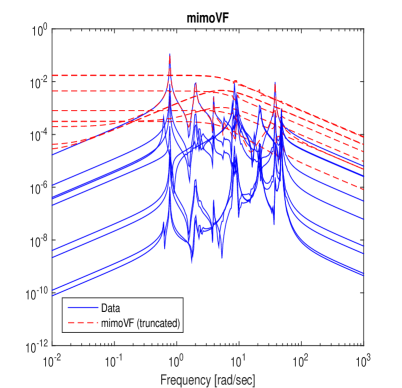
Fig. 7: (Example 5.1.) Illustration of the truncation of mimoVF and the ALS correction. (Truncation applied to the mimoVF output shown on the right graph on Figure 4. Only one ALS iteration is used.) The relative $\mathcal{H}_{2}$ error of $\widehat{{\mathbf{H}}}_{r}$ is $\chi\approx 1.50e-01$.

5.2 Rank-one residue correction via $\mathcal{H}_{2}/\mathcal{H}_{\infty}$ model reduction approaches

The ALS iteration described above is built purely upon algebraic least squares error minimization. However, if the underlying context relates the rational approximants to dynamical systems, then it may be advantageous to perform this reduction using well-developed systems-theoretic reduction tools. Recasting our rank-one residue correction problem into this setting, we consider constructing an $r$-th order system $\widehat{{\mathbf{H}}}_{r}$ that closely approximates the VF computed model ${\mathbf{H}}_{r}$ in some appropriate system norm.

The $\mathcal{H}_{2}$ norm discussed in §4 is the most natural choice and the first one we consider. This approach is compelling when weights and nodes in mimoVF are chosen using an appropriate quadrature as in §4 and the algebraic LS measure is viewed as a discretized $\mathcal{H}_{2}$ measure. In this case, the complete procedure; both mimoVF step and reduction to true McMillan degree-$r$ will be performed with the $\mathcal{H}_{2}$ system norm in mind. To achieve this goal, i.e., to minimize $\|{\mathbf{H}}_{r}-\widehat{{\mathbf{H}}}_{r}\|_{\mathcal{H}_{2}}$ over all stable $r$th order $\widehat{{\mathbf{H}}}_{r}$, we will apply the optimal $\mathcal{H}_{2}$ approximation method IRKA of [33] as modified in [7] for a realization independent procedure. Note that the output of mimoVF, ${\mathbf{H}}_{r}(s)$, has the McMillan degree up to $r\min(p,m)$; thus ${\mathbf{H}}_{r}(s)$ can have a modest state-space dimension. If, for example, $r=80$ and $m=p=50$, ${\mathbf{H}}_{r}$ can have degree as high as $4000$. Thus, it is important to perform this second reduction step effectively. A particularly attractive aspect of the IRKA framework of [7] is that it needs only function and derivative evaluations at dynamically generated points. This works perfectly in our setting since the explicit state-space form of the mimoVF output in (5.1) makes these computations trivial. This approach can be viewed as a data driven implementation of the IRKA – the measurements are fed into mimoVF to produce an intermediate model, a surrogate of the order $\widetilde{r}\geq r$, based on measurements, and then this intermediate model is reduced by IRKA to its locally best $r$th order approximant.

The $\mathcal{H}_{\infty}$ norm is another commonly used system norm. For a stable dynamical system with transfer function ${\mathbf{H}}(s)$, the $\mathcal{H}_{\infty}$ norm is defined as ${\|{\mathbf{H}}\|_{\mathcal{H}_{\infty}}=\sup_{\omega\in{\mathbb{R}}}\|{\mathbf{H}}({\dot{\imath\mskip-3.0mu\imath}}\omega)\|_{2}}$. For details, we refer the reader to [57]. The commonly used approach to model reduction towards obtaining a small $\mathcal{H}_{\infty}$ error measure is Balanced Truncation (BT) [47, 49]. Even though BT requires solving two Lyapunov equations, once again particular state space realization in (5.1) allows straightforward solution of the Lyapunov equations and makes the BT related computations cheap. Thus, we may also employ BT in reduction to true McMillan degree-$r$ without much additional computational cost.

5.3 An aggregate procedure: mimoFIT

Our overall approach to adapting VF to matrix-valued rational approximation consists first of the mimoVF process (described in detail in §2 and §3), followed by a post-processing step that performs the reduction to true McMillan degree-$r$ with minimal loss of fidelity. This post processing stage can be performed either by the ALS correction of §5.1 or by systems-theoretic approaches such as IRKA or BT as described in §5.2. We will refer to this two-step process as mimoFIT.

Numerical Examples

Here, we illustrate the performance of mimoFIT with four numerical examples. In each case, we investigate the effect of the methodology employed in the post-processing stage on the overall approximation quality. We also compare the final models produced by mimoFIT with the optimal-$\mathcal{H}_{2}$ approximations obtained by IRKA.

5.3.1 Heat Model

We consider the Heat Model from the NICONET Benchmark collection [13]; the model has $m=2$ inputs and $p=2$ outputs. We use only $20$ function evaluations ($\ell=40$ samples due to complex conjugacy) and obtain rational approximations of order $r=6$ and $r=10$. Table 2 lists the resulting relative $\mathcal{H}_{2}$ errors due to different approaches. The first row is the error due to the output of mimoVF. Note that this approximation has order $r\times m=2r$ since it has full-rank residues. This is not our final approximation and is included here as a reference point. We obtain a true degree-$r$ approximant using four different approaches: (i) simple rank-$1$ truncation of the residues by SVD, (ii) ALS correction of §5.1, (iii) IRKA on the degree-$2r$ output of mimoVF to reduce it to degree-$r$ (iv) BT on the degree-$2r$ output of mimoVF to reduce it to degree-$r$. These four methods are labeled, respectively, as mimoFIT-(Trnct), mimoFIT-(ALS), mimoFIT-(IRKA), and mimoFIT-(BT). The first observation is that the simple rank-$1$ truncation of the residues by SVD leads to a high loss of accuracy compared to the ALS correction; this is most apparent in the $r=10$ case where mimoFIT-(Trnct) has one order of magnitude higher error than mimoFIT-(ALS). For both cases, mimoFIT-(IRKA) and mimoFIT-(BT) perform extremely well (especially mimoFIT-(IRKA)) and even with a true degree-$r$ approximant, they almost match the accuracy of the degree-$2r$ mimoVF approximant; i.e., reduction from $2r$ to $r$ causes a negligible loss of accuracy. The last row indicates the relative $\mathcal{H}_{2}$ error associated with the optimal approximant from IRKA. As expected, IRKA yields smaller error; we do not anticipate to beat the continuous optimal approximation via a discretized least-square measure. However, it is important to note that mimoFIT-(IRKA) and mimoFIT-(BT) with only $20$ function evaluation yield results close to those obtained by IRKA; this is especially true for $r=10$.

Method	$r=6$	$r=10$
mimoVF (degree: $2r$)	$1.6530\times 10^{-2}$	$1.0759\times 10^{-3}$
mimoFIT-(Trnct)	$3.7022\times 10^{-2}$	$2.6137\times 10^{-2}$
mimoFIT-(ALS)	$1.8218\times 10^{-2}$	$2.8774\times 10^{-3}$
mimoFIT-(IRKA)	${1.7359\times 10^{-2}}$	$1.1686\times 10^{-3}$
mimoFIT-(BT)	$3.0604\times 10^{-2}$	$1.1591\times 10^{-3}$
IRKA	$8.5566\times 10^{-3}$	$1.0925\times 10^{-3}$

Table 2: The relative $\mathcal{H}_{2}$ errors due to mimoVF, mimoFIT and IRKA. $20$ function evaluations

5.3.2 ISS-1R Module

We repeat the above studies for the ISS 1R module [32] with $m=3$ inputs and $p=3$ outputs. We use $100$ function evaluations ($\ell=200$ samples) and obtain rational approximations of order $r=20$ and $r=30$. Table 3 depicts the resulting relative $\mathcal{H}_{2}$ error values for the same methods used in the previous example in §5.3.1. As in the previous example, both mimoFIT-(IRKA) and mimoFIT-(BT) yield very accurate results and show negligible loss of accuracy in reduction from the intermediate $3r$ approximant to the final degree-$r$ approximant; the order of the mimoVF approximant is reduced three-fold yet not much accuracy is lost. mimoFIT-(IRKA) and mimoFIT-(BT) again yield approximation errors close to that of IRKA. The main difference from the previous case is that in this case even the ALS correction suffers from the loss of accuracy as the simple truncation approach.

Method	$r=20$	$r=30$
mimoVF (degree: $3r$)	$4.6074\times 10^{-2}$	$3.3226\times 10^{-2}$
mimoFIT-(Trnct)	$1.2904\times 10^{-1}$	$1.2508\times 10^{-1}$
mimoFIT-(ALS)	$1.2558\times 10^{-1}$	$1.2223\times 10^{-1}$
mimoFIT-(IRKA)	${7.7305\times 10^{-2}}$	$4.4757\times 10^{-2}$
mimoFIT-(BT)	$7.7457\times 10^{-2}$	$3.3483\times 10^{-2}$
IRKA	$6.7779\times 10^{-2}$	$1.1423\times 10^{-2}$

Table 3: The relative $\mathcal{H}_{2}$ errors due to mimoVF, mimoFIT and IRKA. $100$ function evaluations

5.3.3 ISS-12A Module

We now investigate the larger ISS 12A module [32] with $m=3$ inputs and $p=3$ outputs. We focus on this problem since the underlying system of degree $n=1412$ is very hard to approximate with a lower order system; it presents significant challenges to model reduction, not necessarily from a computation perspective but from an approximation quality perspective. As illustrated in [32], the Hankel singular values decay rather slowly, so to obtain a reduced model with a relative error tolerance of $10^{-3}$, one needs a reduced model of order at least $226$ even using balanced truncation. We use $250$ function evaluation, obtain rational approximations of order $r=80$ using mimoFIT, and compare the result with the continuous optimal approximation IRKA. Table 4 depicts the resulting relative $\mathcal{H}_{2}$ error values. As before, both mimoFIT-(IRKA) and mimoFIT-(BT) show negligible loss of accuracy in reduction from the intermediate $3r$ approximant to the final degree-$r$ approximant and have approximation errors close to that of IRKA. mimoFIT-(Trnct) and mimoFIT-(ALS) perform reasonably well as well in this case with mimoFIT-(Trnct) having the largest error among the four.

Method	$r=80$
mimoVF (degree: $3r$)	$1.4678\times 10^{-1}$
mimoFIT-(Trnct)	$2.4549\times 10^{-1}$
mimoFIT-(ALS)	$2.2075\times 10^{-1}$
mimoFIT-(IRKA)	${1.5116\times 10^{-1}}$
mimoFIT-(BT)	$1.5130\times 10^{-1}$
IRKA	$1.1317\times 10^{-1}$

Table 4: The relative $\mathcal{H}_{2}$ errors due to mimoVF, mimoFIT and IRKA. $250$ function evaluations

5.3.4 A power system example with large input/output space

This example results from small-signal stability studies for large power systems. The specific model we consider here is one of the models from the Brazilian Interconnect Power System (BIPS); refer to [45] for details.

The underlying dynamical system has dimension $n=13250$ with $m=46$ inputs and $p=46$ outputs. We apply mimoFIT-(BT) to obtain our rational approximant. We use $\ell=200$ frequency samples. The mimoVF (first step of mimoFIT) is applied with $r=40$. Due to $m=p=46$, the output of mimoVF has an effective McMillan degree of $r\times m=1840$. Note that this is only marginally a reduced model, having a McMillan degree roughly $14\%$ of the originally system order. The decay of the leading Hankel singular values of the intermediate model is shown in the upper plot of Figure 8. Note the slow decay; even after the $300^{\rm th}$ one, the normalized Hankel singular values are still above the threshold of $10^{-4}$. This system is difficult to reduce. Indeed, in earlier works, even for simpler versions of the model having a smaller number of input and outputs (such as $m=p=28$), a reduced model of degree $291$ was used; see [51]. We choose the final degree to be a point at which the normalized Hankel singular values have decayed below $2\times 10^{-4}$, leading to a final McMillan degree of $253$ (around $2\%$ of the original). The sigma plots, i.e., $\|{\mathbf{H}}({\dot{\imath\mskip-3.0mu\imath}}\omega)\|_{2}$ vs $\omega\in{\mathbb{R}}$, for the full model and the final mimoFIT approximant are shown in the lower plot of Figure 8. As the figure illustrates, the mimoFIT approximant does an excellent job in approximating the underlying dynamics.

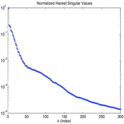
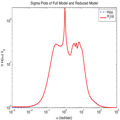
Fig. 8: (Example 5.3.4.) Large-scale power system example: Left plot: Decay of the Hankel singular values Right plot: The sigma plots of the full and reduced model.

6 Conclusions

The VF method, as originated by Gustavsen and Semlyen, has been and continues to be an important tool for rational approximation and many authors have applied, modified, and analyzed this approach. Although their method is based on successive solution of linear LS problems, which are well understood problems in of themselves, we find that subtleties enter that can degrade both the performance and accuracy of current VF approaches, especially for matrix-valued rational approximation of modest dimension which often produce extremely poorly conditioned problems. These issues include

1. balancing the potential conflict between rank revealing pivoting in QR factorizations used in LS solvers and column-scaling used to improve conditioning;

2. avoiding redundant computation within the multiple subproblems solved as part of the large LS problem that arises;

3. the need for rigorous termination criteria and the efficient recovery of the best possible rational approximant in case the iteration must be terminated prematurely;

4. the use of regularized least squares and the discrepancy principle, both implemented using high accuracy linear algebra methods; and

5. control of the McMillan degree of the resulting rational approximant.

In this paper, we have considered these issues carefully, together with other more minor ones. We have integrated these developments into a robust, efficient implementation of VF for matrix-valued rational approximation, called mimoVF, that appears to be both faster and more accurate than currently available implementations. Further, we have connected the underlying discrete LS approximation problem to a continuous optimal $\mathcal{H}_{2}$ approximation problem through numerical quadrature, which motivated a reformulation of the original VF objective as a weighted LS problem. For essentially the same cost as mimoVF, we were then able to use this reformulation to significantly improve the quality of the approximation. Finally, we have offered here an aggregate procedure, called mimoFIT, that combines mimoVF with $\mathcal{H}_{2}$/$\mathcal{H}_{\infty}$-based approximation methods that yield high-fidelity rational approximants with low McMillan degree.

References

- [1] E. Anderson, Z. Bai, C. Bischof, L. S. Blackford, J. Demmel, J. J. Dongarra, J. Du Croz, S. Hammarling, A. Greenbaum, A. McKenney, and D. Sorensen, LAPACK Users’ Guide (Third Ed.), Society for Industrial and Applied Mathematics, Philadelphia, PA, USA, 1999.
- [2] A. Antoulas, Approximation of Large-Scale Dynamical Systems (Advances in Design and Control), Society for Industrial and Applied Mathematics, Philadelphia, PA, USA, 2005.
- [3] , Model reduction of nonlinear systems in the Loewner framework, in Proceedings of the 21st International Symposium on Mathematical Theory of Networks and Systems, 2014.
- [4] , Data-driven model reduction for weakly nonlinear systems: A summary, in Proceedings of the 8th Vienna International Conference on Mathematical Modeling, 2015.
- [5] A. Antoulas, C. Beattie, and S. Gugercin, Interpolatory model reduction of large-scale dynamical systems, in Efficient Modeling and Control of Large-Scale Systems, J. Mohammadpour and K. Grigoriadis, eds., Springer-Verlag, 2010, pp. 2–58.
- [6] A. Antoulas, A. Ionita, and S. Lefteriu, On two-variable rational interpolation, Linear Algebra and Its Applications, 436 (2012), pp. 2889–2915.
- [7] C. Beattie and S. Gugercin, Realization–independent approximation, in Proceedings of the 51st IEEE Conference on Decision & Control, IEEE, 2012, pp. 4953–4958.
- [8] P. Benner, S. Gugercin, and K. Willcox, A survey of model reduction methods for parametric systems, Tech. Rep. MPIMD/13-14, Max Planck Institute Magdeburg, August 2013.
- [9] A. R. Benson, D. F. Gleich, and J. Demmel, Direct QR factorizations for tall-and-skinny matrices in mapreduce architectures, CoRR, abs/1301.1071 (2013).
- [10] J. P. Boyd, Exponentially convergent Fourier-Chebshev quadrature schemes on bounded and infinite intervals, Journal on Scientific Computing, 2 (1987), pp. 99–109.
- [11] P. A. Businger and G. H. Golub, Linear least squares solutions by Householder transformations, Numerische Mathematik, 7 (1965), pp. 269–276.
- [12] N. Castro-González, J. Ceballos, F. M. Dopico, and J. M. Molera, Accurate solution of structured least squares problems via rank-revealing decompositions, SIAM J. Matrix Analysis Applications, 34 (2013), pp. 1112–1128.
- [13] Y. Chahlaoui and P. V. Dooren, A collection of benchmark examples for model reduction of linear time invariant dynamical systems, tech. rep., SLICOT Working Note 2002-2, 2002.
- [14] A. Chinea and S. Grivet-Talocia, On the parallelization of Vector Fitting algorithms, IEEE Transactions on Components, Packaging and Manufacturing Technology, 1 (2011), pp. 1761–1773.
- [15] A. J. Cox and N. J. Higham, Stability of Householder QR factorization for weighted least squares problems, in Numerical Analysis 1997, Proceedings of the 17th Dundee Biennial Conference, D. F. Griffiths, D. J. Higham, and G. A. Watson, eds., vol. 380 of Pitman Research Notes in Mathematics, A W Longman, 1998, pp. 57–73.
- [16] J. Demmel, Accurate singular value decompositions of structured matrices, SIAM J. Matrix Anal. Appl., 21 (1999), pp. 562–580.
- [17] J. Demmel, L. Grigori, M. Gu, and H. Xiang, Communication avoiding rank revealing QR factorization with column pivoting, Tech. Rep. UCB/EECS-2013-46, EECS Department, University of California, Berkeley, May 2013.
- [18] J. Demmel, M. Gu, S. Eisenstat, I. Slapničar, K. Veselić, and Z. Drmač, Computing the singular value decomposition with high relative accuracy, Lin. Alg. Appl., 299 (1999), pp. 21–80.
- [19] D. Deschrijver, B. Gustavsen, and T. Dhaene, Advancements in iterative methods for rational approximation in the frequency domain, Power Delivery, IEEE Transactions on, 22 (2007), pp. 1633–1642.
- [20] D. Deschrijver, B. Haegeman, and T. Dhaene, Orthonormal vector fitting: a robust macromodeling tool for rational approximation of frequency domain responses, IEEE Transactions on Advanced Packaging, 30 (2007), pp. 216–225.
- [21] D. Deschrijver, L. Knockaert, and T. Dhaene, Improving robustness of vector fitting to outliers in data, Electronics Letters, 46 (2010), pp. 1–2.
- [22] D. Deschrijver, M. Mrozowski, T. Dhaene, and D. D. Zutter, Macromodeling of multiport systems using a fast implementation of the vector fitting method, IEEE Microwave and Wireless Components Letters, 18 (2008), pp. 383–385.
- [23] , A barycentric vector fitting algorithm for efficient macromodeling of linear multiport systems, IEEE Microwave and Wireless Components Letters, 23 (2013), pp. 60–62.
- [24] Z. Drmač, On principal angles between subspaces of Euclidean space, SIAM J. Matrix Anal. Appl., 22 (2000), pp. 173–194.
- [25] Z. Drmač and Z. Bujanović, On the failure of rank revealing QR factorization software – a case study, ACM Trans. Math. Softw., 35 (2008), pp. 1–28.
- [26] Z. Drmač, S. Gugercin, and C. Beattie, Quadrature-based vector fitting for discretized approximation, SIAM J. Sci. Comp. (to appear), (2014).
- [27] Z. Drmač and K. Veselić, New fast and accurate Jacobi SVD algorithm: I., SIAM J. Matrix Anal. Appl., 29 (2008), pp. 1322–1342.
- [28] , New fast and accurate Jacobi SVD algorithm: II., SIAM J. Matrix Anal. Appl., 29 (2008), pp. 1343–1362.
- [29] G. Golub, V. Klema, and S. C. Peters, Rules and software for detecting rank degeneracy, Journal of Econometrics, 12 (1980), pp. 41 – 48.
- [30] G. H. Golub, V. C. Klema, and G. W. Stewart, Rank degeneracy and least squares problems, tech. rep., Stanford, CA, USA, 1976.
- [31] P. Gonnet, R. Pachón, and L. N. Trefethen, Robust rational interpolation and least-squares, Electronic Transactions on Numerical Analysis, 38 (2011), pp. 146–167.
- [32] S. Gugercin, A. Antoulas, and N. Bedrossian, Approximation of the international space station 1r and 12a models, in Decision and Control, 2001. Proceedings of the 40th IEEE Conference on, vol. 2, IEEE, 2001, pp. 1515–1516.
- [33] S. Gugercin, A. C. Antoulas, and C. Beattie, model reduction for large-scale linear dynamical systems, SIAM J. Matrix Anal. Appl., 30 (2008), pp. 609–638.
- [34] B. Gustavsen, Comments on “a comparative study of vector fitting and orthonormal vector fitting techniques for EMC applications”, in Proceedings of the 18th Int. Zurich Symposium on Electromagnetic Compatibility, Munich 2007, IEEE, 2006, pp. 131–134.
- [35] , Improving the pole relocating properties of vector fitting, IEEE Transactions on Power Delivery, 21 (2006), pp. 1587–1592.
- [36] B. Gustavsen and A. Semlyen, Rational approximation of frequency domain responses by vector fitting, IEEE Transactions on Power Delivery, 14 (1999), pp. 1052–1061.
- [37] , A robust approach for system identification in the frequency domain, IEEE Transactions on Power Delivery, 19 (2004), pp. 1167–1173.
- [38] W. Hendrickx and T. Dhaene, A discussion of “Rational approximation of frequency domain responses by vector fitting”, IEEE Transactions on Power Systems, 21 (2006), pp. 441–443.
- [39] N. J. Higham, QR factorization with complete pivoting and accurate computation of the SVD, Linear Algebra and its Applications, 309 (2000), pp. 153–174.
- [40] J. Hokanson, Numerically Stable and Statistically Efficient Algorithms for Large Scale Exponential Fitting, PhD thesis, Doctoral Thesis, Rice University. http://hdl. handle. net/1911/77161, 2013.
- [41] A. Ionita and A. Antoulas, Data-driven parametrized model reduction in the Loewner framework, SIAM Journal on Scientific Computing, 36 (2014), pp. A984–A1007.
- [42] R. E. Kalman, Design of a self-optimizing control system, Trans. ASME, 80 (1958), pp. 468–478.
- [43] C. L. Lawson and R. J. Hanson, Solving least squares problems, vol. 161, SIAM, 1974.
- [44] S. Lefteriu and A. Antoulas, A new approach to modeling multiport systems from frequency-domain data, Computer-Aided Design of Integrated Circuits and Systems, IEEE Transactions on, 29 (2010), pp. 14–27.
- [45] N. Martins, P. Pellanda, and J. Rommes, Computation of transfer function dominant zeros with applications to oscillation damping control of large power systems, Power Systems, IEEE Transactions on, 22 (2007), pp. 1657–1664.
- [46] A. J. Mayo and A. C. Antoulas, A framework for the solution of the generalized realization problem, Linear Algebra and its Applications, 425 (2007), pp. 634–662.
- [47] B. Moore, Principal component analysis in linear systems: Controllability, observability, and model reduction, Automatic Control, IEEE Transactions on, 26 (1981), pp. 17–32.
- [48] V. Morozov, On the solution of functional equations by the method of regularization, Soviet Mathematics Doklady, 7 (1966), pp. 414–417.
- [49] C. Mullis and R. Roberts, Synthesis of minimum roundoff noise fixed point digital filters, Circuits and Systems, IEEE Transactions on, 23 (1976), pp. 551–562.
- [50] M. J. D. Powell and J. K. Reid, On applying Householder transformations to linear least squares problems, in Information Processing 68, Proc. International Federation of Information Processing Congress, Edinburgh, 1968, North Holland, Amsterdam, 1969, pp. 122–126.
- [51] J. Rommes and N. Martins, Efficient computation of multivariable transfer function dominant poles using subspace acceleration, Power Systems, IEEE Transactions on, 21 (2006), pp. 1471–1483.
- [52] C. Sanathanan and J. Koerner, Transfer function synthesis as a ratio of two complex polynomials, IEEE Trans. Autom. Control, 8 (1963), pp. 56–58.
- [53] W. Schilders, H. van der Vorst, and J. Rommes, Model order reduction: theory, research aspects and applications, vol. 13, Springer, 2008.
- [54] Sintef, VFIT3. http://www.sintef.no/Projectweb/VECTFIT/Downloads/VFUT3/.
- [55] A. Sluis, Condition numbers and equilibration of matrices, Numerische Mathematik, 14 (1969), pp. 14–23.
- [56] G. W. Stewart, Determining rank in the presence of error, in Linear algebra for large scale and real-time applications (Proceedings of the NATO Advanced Study Institute, Leuven, Belgium, August 3-14, 1992), M. S. Moonen, G. H. Golub, and B. L. de Moor, eds., Kluwer Academic Publishers, 1993, pp. 275–291.
- [57] K. Zhou, J. Doyle, and K. Glover, Robust and Optimal Control, Prentice-Hall, 1996.