Adaptive estimation of the baseline hazard function in the Cox model by model selection, with high-dimensional covariates

Abstract

The purpose of this article is to provide an adaptive estimator of the baseline function in the Cox model with high-dimensional covariates. We consider a two-step procedure : first, we estimate the regression parameter of the Cox model via a Lasso procedure based on the partial log-likelihood, secondly, we plug this Lasso estimator into a least-squares type criterion and then perform a model selection procedure to obtain an adaptive penalized contrast estimator of the baseline function.

Using non-asymptotic estimation results stated for the Lasso estimator of the regression parameter, we establish a non-asymptotic oracle inequality for this penalized contrast estimator of the baseline function, which highlights the discrepancy of the rate of convergence when the dimension of the covariates increases.

Keywords: Survival analysis; Conditional hazard rate function; Cox’s proportional hazards model; Right-censored data; Semi-parametric model; Nonparametric model; High-dimensional covariates; Model selection; Non-asymptotic oracle inequalities; Concentration inequalities

1 Introduction

Consider the following Cox model, introduced by Cox (1972) and defined, for a vector of covariates $\boldsymbol{Z}=(Z_{1},...,Z_{p})^{T}$, by

$$\lambda_{0}(t,\boldsymbol{Z})=\alpha_{0}(t)\exp(\boldsymbol{\beta_{0}^{T}Z}),$$ (1)

where $\lambda_{0}$ denotes the hazard rate, $\boldsymbol{\beta_{0}}=(\beta_{0_{1}},...,\beta_{0_{p}})^{T}\in\mathbb{R}^{p}$ is the regression parameter and $\alpha_{0}$ is the baseline hazard function. The Cox partial log-likelihood, introduced by Cox (1972), allows to estimate $\boldsymbol{\beta_{0}}$ without the knowledge of $\alpha_{0}$, considered as a functional nuisance parameter. For the estimation of $\alpha_{0}$, one common way is to use a two step procedure, starting with the estimation of $\boldsymbol{\beta_{0}}$ alone and then to plug this estimator into a non parametric type estimator $\alpha_{0}$, usually a kernel type estimator.

Let us be more specific.

When $p$ is small compared to $n$, $\boldsymbol{\beta_{0}}$ is usually estimated by minimization of the opposite of the Cox partial log-likelihood. We refer to Andersen et al. (1993), as a reference book, for the proofs of the consistency and the asymptotic normality of $\boldsymbol{\hat{\beta}}$ when $p$ is small compared to $n$. Thoses strategies only apply when $p<n$ and even more, they only apply when $p$ is small compared to $n$. When $p$ growths up, becoming of the same order as $n$ and possibly larger than $n$, various well known problems appears. Among them, the minimization of the opposite of the Cox partial log-likelihood becomes difficult and even impossible if $p>n$.

In high-dimension, when $p$ is large compared to $n$, the Lasso procedure is one of the classical considered strategies. The Lasso (Least Absolute Shrinkage and Selection Operator) has been first introduced by Tibshirani (1996) in the linear regression model. It has been largely considered in additive regression model (see for instance Knight and Fu (2000), Efron et al. (2004), Donoho et al. (2006), Meinshausen and Bühlmann (2006), Zhao and Yu (2006), Zhang and Huang (2008), Meinshausen and Yu (2009) and also Juditsky and Nemirovski (2000), Nemirovski (2000), Bunea et al. (2006; 2007a; 2007b), Greenshtein and Ritov (2004) or Bickel et al. (2009)), and in density estimation (see Bunea et al. (2007c) and Bertin et al. (2011)). In the particular case of the semi-parametric Cox model, Tibshirani (1997) has proposed a Lasso procedure for the regression parameter. The Lasso estimator of the regression parameter $\boldsymbol{\hat{\beta}}$ is defined as the minimizer of the opposite of the Cox partial log-likelihood under an $\ell_{1}$ type constraint, that is, suitably penalized with an $\ell_{1}$-penalty function. Recent results exist on the estimation of $\boldsymbol{\beta_{0}}$ in high-dimension setting. Among them one can mention Bradic et al. (2012) who have proved asymptotic results for Lasso estimator. More recently, Bradic and Song (2012), Kong and Nan (2012) and Huang et al. (2013) establish the first non-asymptotic oracle inequalities (estimation and prediction bounds) for the Lasso estimator.

For the baseline hazard function and when $p$ is small compared to $n$, the common estimator is a kernel estimator, which depends on $\boldsymbol{\hat{\beta}}$ obtained by minimization of the opposite of the Cox partial log-likelihood. This kernel estimator has been introduced by Ramlau-Hansen (1983a; b) from the Breslow estimator of the cumulative baseline function (see Ramlau-Hansen (1983b) and Andersen et al. (1993) for more details). In this context, Ramlau-Hansen (1983b) and Grégoire (1993) proved asymptotic results. No non-asymptotic results and no adaptive results have to date been established for the kernel estimator of the baseline function. Finally, when $p$ is large compared to $n$, to our knowledge, the construction of an estimator of the baseline function has not been yet considered.

In this paper, we consider a two-step procedure to estimate $\boldsymbol{\beta_{0}}$ and $\alpha_{0}$, the two parameters in the Cox model. But our contributions focus more on the estimation of $\alpha_{0}$. In the Cox model we consider, it is noteworthy that the high-dimension only concerns the regression parameter, whereas the baseline function is a time function. Its estimation would not require a procedure specific to high-dimension, besides the first step concerning the estimation of $\boldsymbol{\beta_{0}}$. We propose a procedure for the construction of an estimator of the baseline hazard function $\alpha_{0}$, $p$ being either smaller than $n$ or greater than $n$. It combines a Lasso procedure for $\boldsymbol{\beta_{0}}$ as a first step and a second step based on a model selection strategy for the estimation of the baseline function $\alpha_{0}$. This model selection procedure takes its origins in the works of Akaike (1973) and Mallows (1973), more recently formalized by Birgé and Massart (1997) and Barron et al. (1999) for the estimation of densities and regression functions (see the book of Massart (2007) as a reference work on model selection). In survival analysis, the model selection has also been documented. Letué (2000) has adapted these methods to estimate the regression function of the non-parametric Cox model, when $p<n$. More recently, Brunel and Comte (2005), Brunel et al. (2009), Brunel et al. (2010) have obtained adaptive estimation of densities in a censoring setting. Model selection methods have also been used to estimate the intensity function of a counting process in the multiplicative Aalen intensity model (see Reynaud-Bouret (2006) and Comte et al. (2011)). However, the model selection procedure has never been considered, to our knowledge, for estimating the baseline hazard function in the Cox model.

Our contributions are at least threefold: Our procedure is the first that focus on the estimation of baseline function of the semi-parametric Cox model with high-dimentional covariates. This procedure provide an adaptive estimator of the baseline function that works as well for small $p$ and large $p$ compared to $n$ (that is for possibly high-dimensional covariates). Furthermore, for this estimator, we state non-asymptotic oracle inequalities, that hold, once again, $p$ being either smaller than $n$ or greater than $n$. More precisely, we prove that the risk of this estimator achieves the best risk among estimators in a large collection. For each model, the risk of an estimator is bounded by the sum of three terms. The first term is a bias term involving to the approximation properties of the collection of models, through the distance evaluated in $\boldsymbol{\beta_{0}}$ between the true baseline and the orthogonal projection of $\alpha_{0}$ on the best selected model. The second term is a penalty term of the same order than the variance on one model, that is of order the dimension of one model over $n$, as expected with $\ell_{0}$-penalty. These two terms are the "usual" terms appearing in nonparametric estimation. It is noteworthy that these two terms do not involve any quantity related to the risk of the Lasso estimator of $\boldsymbol{\beta_{0}}$. The last term precisely comes from the properties of the Lasso estimator of $\boldsymbol{\beta_{0}}$. This last term is of order $\log(np)/n$, as expected for a Lasso estimator.

When $p$ is small, the third last term is of order $\log(n)/n$ and, the rate is governed by the first two terms. In that case, the penalty term being of the same order than the variance over one model, we conclude that the model selection procedure achieves the "expected rate" of order $n^{-2\gamma/(2\gamma+1)}$ when the baseline function belongs to a Besov space with smoothness parameter $\gamma$. This continues to hold when $p$ is of the same order than the sample size $n$. When $p$ is larger than $n$, that is in the so-called ultra-high dimension (see Verzelen (2012)), the rate for estimating $\alpha_{0}$ is changed, and more precisely degraded as a price to pay for being with high dimension covariates. This degradation follows accordingly to the order of $p$ compared to $n$.

The main tools for stating our results are the theory of marked counting processes and martingales with jumps, the theory of penalized minimum contrast estimators and concentrations inequalities such as Talagrand inequality (see Talagrand (1996)) and a Bernstein inequality found in (see van de Geer (1995) and Comte et al. (2011)) for unbounded martingale process and combined with chaining methods (see Talagrand (2005) and Baraud (2010)).

The article is organized as follows. In Section 3, we describe the estimation procedure. Section 4 provides non-asymptotic oracle inequalities on the estimator of the baseline hazard function $\alpha_{0}$, in a high-dimensional setting for $\boldsymbol{\beta_{0}}$. In section 5, we compare the performances of the resulting penalized contrast estimator to those of the usual kernel estimator on simulated data. Section 6 is devoted to the proofs: we state some technical results, then we establish the two main theorems and lastly we prove the technical results. Finally, Appendix A discusses the bound of the error estimation for the Lasso estimator of the regression parameter of the Cox model.

2 Notations and preliminaries

2.1 Framework with counting processes

Consider the general setting of counting processes, which embeds the classical case of right censoring. We follow here the now classical setting of Andersen et al. (1993) or Fleming and Harrington (2011). For $n$ independant individuals, we observe for $i=1,...,n$ a counting process $N_{i}$, a random process $Y_{i}$ with values in $[0,1]$ and a vector of covariates $\boldsymbol{Z_{i}}=(Z_{i,1},...,Z_{i,p})^{T}\in\mathbb{R}^{p}$. Let $(\Omega,\mathcal{F},\mathbb{P})$ be a probability space and $(\mathcal{F}_{t})_{t\geq 0}$ be the filtration defined by

$$\mathcal{F}_{t}=\sigma\{N_{i}(s),Y_{i}(s),0\leq s\leq t,\boldsymbol{Z_{i}},i=1,...,n\}.$$

From the Doob-Meyer decomposition, we know that each $N_{i}$ admits a compensator denote by $\Lambda_{i}$, such that $M_{i}=N_{i}-\Lambda_{i}$ is a $(\mathcal{F}_{t})_{t\geq 0}$ local square-integrable martingale (see Andersen et al. (1993) for details). We assume in the following that $N_{i}$ has a satisfies an Aalen multiplicative intensity model.

Assumption 2.1.

For each $i=1,...,n$ and all $t\geq 0$,

$$\Lambda_{i}(t)=\displaystyle{\int_{0}^{t}\lambda_{0}(s,\boldsymbol{Z_{i}})Y_{i}(s)\mathrm{d}s},$$ (2)

where $\lambda_{0}(t,\boldsymbol{z})=\alpha_{0}(t){\mathrm{e}}^{\boldsymbol{\beta^{T}z}}$, for $\boldsymbol{z}\in\mathbb{R}^{p}$.

We observe the independent and identically distributed (i.i.d.) data $(\boldsymbol{Z_{i}},N_{i}(t),Y_{i}(t),i=1,...,n,0\leq t\leq\tau)$, where $[0,\tau]$ is the time interval between the beginning and the end of the study.

This general setting, introduced by Aalen (1980), embeds several particular examples as censored data, marked Poisson processes and Markov processes (see Andersen et al. (1993) for further details). We give here details for the right censoring case. We observe for $i=1,...,n$, $(X_{i},\delta_{i},\boldsymbol{Z_{i}})$, where $X_{i}=\min({T_{i}},{C_{i}})$, $\delta_{i}=\mathds{1}_{\{T_{i}\leq C_{i}\}}$, $T_{i}$ is the time of interest and $C_{i}$ the censoring time. With these notations, the $(\mathcal{F}_{t})_{t\geq 0}$-adapted processes $Y_{i}$ and $N_{i}$ are respectively defined as the at-risk process $Y_{i}(t)=\mathds{1}_{\{X_{i}\geq t\}}$ and the counting process $N_{i}(t)=\mathds{1}_{\{X_{i}\leq t,\delta_{i}=1\}}$ which jumps when the ith individual dies.

2.2 Assumptions

Before describing the estimation procedure, we introduce few assumptions on the framework defined in Subsection 2.1.

Let $\boldsymbol{Z}\in\mathbb{R}^{p}$ denote the generic vector of covariates with the same distribution as the vectors of covariates $\boldsymbol{Z_{i}}$ of each individual $i$ and by $Z_{j}$ its $j$-th component, namely the $j$-th covariates of the vector $\boldsymbol{Z}$. Similarly, we denote by $Y$ the generic version of the random process $Y_{i}$ with values in $[0,1]$.

We define the standard $\mathbb{L}^{2}$ and $\mathbb{L}^{\infty}$-norms, for $\alpha\in(\mathbb{L}^{2}\cap\mathbb{L}^{\infty})([0,\tau])$:

$$||\alpha||^{2}_{2}=\displaystyle\int_{0}^{\tau}\alpha^{2}(t)\mathrm{d}t\quad\mbox{and}\quad||\alpha||_{\infty,\tau}=\underset{t\in[0,\tau]}{\sup}|\alpha(t)|.$$

For a vector $\boldsymbol{b}\in\mathbb{R}^{p}$, we also introduce the $\ell_{1}$-norm $|b|_{1}=\sum_{j=1}^{p}|b_{j}|$.

Assumption 2.2.

1. There exists a positive constant $B$ such that

   $$|Z_{j}|\leq B,\quad\forall j\in\{1,...,p\}.$$

   In the following, we denote $A=[-B,B]^{p}$.

2. The vector of covariates $\boldsymbol{Z}$ admit a p.d.f. $f_{\boldsymbol{Z}}$ such that $\sup_{A}|f_{\boldsymbol{Z}}|\leq f_{1}<+\infty$.

3. There exists $f_{0}>0$, such that $\forall(t,\boldsymbol{z})\in[0,\tau]\times A$,

   $$\mathbb{E}[Y(t)|\boldsymbol{Z}=\boldsymbol{z}]f_{\boldsymbol{Z}}(\boldsymbol{z})\geq f_{0}.$$

4. For all $t\in[0,\tau]$, $\alpha_{0}(t)\leq||\alpha_{0}||_{\infty,\tau}<+\infty$.
   

Remark 2.3.

Let say a few word on these assumptions starting by noting that these four assumptions are quite classic and reasonnable. To be more specific, Assumption 2.2.(i), is very common to establish oracle inequalities of Lasso estimators in various frameworks. In particular, in the Cox model, see e.g. Huang et al. (2013) and Bradic and Song (2012) for the statement of non asymptotic oracle inequalities

In the specific case of right censoring, Assumption 2.2.(iii) is automatically verified. Indeed, for $T$ the survival time and $C$ the censoring time, we can write

$$\mathbb{E}(Y(t)|\boldsymbol{Z}=\boldsymbol{z})=\mathbb{E}(\mathds{1}_{\{T\wedge C\leq t\}}|\boldsymbol{Z}=\boldsymbol{z})=(1-F_{T|\boldsymbol{Z}}(t))(1-G_{C|\boldsymbol{Z}}(t-)),$$

where $F_{T|\boldsymbol{Z}}$ and $G_{C|\boldsymbol{Z}}$ are the cumulative distribution functions of $T|\boldsymbol{Z}$ and $C|\boldsymbol{Z}$ respectively. It is known (see Andersen et al. (1993)) that the Kaplan-Meier estimator is consistent only on intervals of the form $[0,\tau]$, where $\tau\leq\sup\{t\geq 0,(1-F_{T|\boldsymbol{Z}}(t))(1-G_{C|\boldsymbol{Z}}(t))>0\}$. Hence when $f_{\boldsymbol{Z}}$ is bounded from below on $A$, there exists $f_{0}>0$, such that

$$\forall(t,\boldsymbol{z})\in[0,\tau]\times A,\quad\mathbb{E}[Y(t)|\boldsymbol{Z}=\boldsymbol{z}]f_{\boldsymbol{Z}}(\boldsymbol{z})\geq f_{0}.$$

Assumption 2.2.(iii) is required in order to compare the natural norm of the baseline function induced by our contrast to the standard $\mathbb{L}^{2}$-norm (see Proposition 6.1).

3 Estimation procedure

We now describe our two-steps estimation procedure, starting by recalling the Lasso estimation of $\boldsymbol{\beta_{0}}$ and then giving a bound of its prediction risk. Then, we describe the contrast and the model selection procedure for the estimation of the baseline function.

3.1 Preliminary estimation of $\boldsymbol{\beta_{0}}$: procedure and results

The Lasso estimator $\boldsymbol{\hat{\beta}}$ of the regression parameter $\boldsymbol{\beta_{0}}$, introduced in Tibshirani (1997), is defined by

$$\boldsymbol{\hat{\beta}}=\underset{\boldsymbol{\beta}\in\mathbb{R}^{p}}{\arg\min}\{-l^{*}_{n}(\boldsymbol{\beta})+\Gamma_{n}|\boldsymbol{\beta}|_{1}\},$$ (3)

where $\Gamma_{n}$ is a positive regularization parameter to be suitable chosen, $|\boldsymbol{\beta}|_{1}=\sum_{j=1}^{p}|\beta_{j}|$ and $l^{*}_{n}$ is the Cox partial log-likelihood defined by,

$$l^{*}_{n}(\boldsymbol{\beta})=\dfrac{1}{n}\displaystyle\sum_{i=1}^{n}\displaystyle\int_{0}^{\tau}\log\dfrac{{\mathrm{e}}^{\boldsymbol{\beta^{T}Zi}}}{S_{n}(t,\boldsymbol{\beta})}\mathrm{d}N_{i}(t),\quad\mbox{where }S_{n}(t,\boldsymbol{\beta})=\dfrac{1}{n}\displaystyle\sum_{i=1}^{n}{\mathrm{e}}^{\boldsymbol{\beta^{T}Z_{i}}}Y_{i}(t)\quad\forall t\geq 0.$$ (4)

The risk bounds for the estimator of $\alpha_{0}$ will naturally involve the risk $|\boldsymbol{\hat{\beta}}-\boldsymbol{\beta_{0}}|_{1}$, that have to be at least bounded. Thus, we rather consider the following procedure

$$\boldsymbol{\hat{\beta}}=\underset{\boldsymbol{\beta}\in\mathcal{B}(0,R_{1})}{\arg\min}\{-l^{*}_{n}(\boldsymbol{\beta})+\operatorname{pen}(\boldsymbol{\beta})\},\quad\mbox{with}\quad\operatorname{pen}(\boldsymbol{\beta})=\Gamma_{n}|\boldsymbol{\beta}|_{1},$$ (5)

where $\mathcal{B}(0,R_{1})$ is the ball defined by

$$\mathcal{B}(0,R_{1})=\{b\in\mathbb{R}^{p}:|b|_{1}\leq R_{1}\},\quad\mbox{with }R_{1}>0.$$

Consider the following assumption:

Assumption 3.1.

We assume that $|\boldsymbol{\beta_{0}}|_{1}<R_{2}<+\infty$.

We denote $R=\max(R_{1},R_{2})$, so that

$$|\boldsymbol{\hat{\beta}}-\boldsymbol{\beta_{0}}|_{1}\leq 2R\quad\mbox{ a.s}.$$ (6)

Such condition has already been considered by van de Geer (2008) or Kong and Nan (2012). Roughly speaking, it means that we can restrict our attention to a ball, possibly very large, in a neighborhood of $\boldsymbol{\beta_{0}}$ for finding a good estimator of $\boldsymbol{\beta_{0}}$.

As mentionned above, our risk bounds for the estimator of $\alpha_{0}$ depend on the risk $|\boldsymbol{\hat{\beta}}-\boldsymbol{\beta_{0}}|_{1}$. Such bounds on this risk already exist. In particular, in their Theorem 3.1, Huang et al. (2013) state a non asymptotic inequality for $|\boldsymbol{\hat{\beta}}-\boldsymbol{\beta_{0}}|_{1}$ in the specific case of bounded counting processes. We consider here more general processes, possibly unbounded. In the following proposition, we provide a generalization of the results established by Huang et al. (2013) to the case of unbounded counting processes. We refer to Appendix A for a proof of Proposition 3.2.

Proposition 3.2.

Let $k>0$, $c>0$ and $s:=\operatorname{Card}\{j\in\{1,...,p\}:\beta_{0_{j}}\neq 0\}$ be the sparsity index of $\boldsymbol{\beta_{0}}$. Assume that $||\alpha_{0}||_{\infty,\tau}<\infty$. Then, under Assumptions 3.1 and (i), with probability larger than $1-cn^{-k}$, we have

$$|\boldsymbol{\hat{\beta}}-\boldsymbol{\beta_{0}}|_{1}\leq C(s)\sqrt{\dfrac{\log(pn^{k})}{n}}$$ (7)

where $C(s)>0$ is a constant depending on the sparsity index $s$.

As mentioned previously, this proposition is crucial to establish a non-asymptotic oracle inequality for the baseline function. In the rest of the paper, we consider that $\boldsymbol{\hat{\beta}}$ satisfies Inequality (7).

Assumption 3.3.

We assume that

$$\underset{n\rightarrow\infty}{\lim}C(s)\dfrac{\log(np)}{n}=0.$$

This assumption is clearly reasonable: when $p$ is smaller than $n$ or of the same order, this assumption is automatically fulfilled. It is not satisfied when $p$ becomes too high compared to $n$. This case corresponds to the now well known case of ultra-high dimension framework. In this specific case, recent lower bounds in additive regression models typically say that the estimation of paramater is mostly impossible (see for example Verzelen (2012)).

3.2 Estimation of $\alpha_{0}$

We now come to the estimation of the baseline function $\alpha_{0}$ via a model selection procedure. As usual, such a procedure requires an empirical estimation criterion, a collection of models and a suitable penalty function, all being presented in the following.

3.2.1 Definition of the estimation criterion

We estimate the baseline function $\alpha_{0}$ using a least-squares criterion. More precisely, based on the data $(\boldsymbol{Z_{i}},N_{i}(t),Y_{i}(t),i=\leavevmode\nobreak\ 1,...,n,0\leq\leavevmode\nobreak\ t\leq\tau)$ and for a fixed $\boldsymbol{\beta}$, we consider the empirical least-squares type given for a function $\alpha\in(\mathbb{L}^{2}\cap\mathbb{L}^{\infty})([0,\tau])$ by

$$C_{n}(\alpha,\boldsymbol{\beta})=-\dfrac{2}{n}\displaystyle{\sum_{i=1}^{n}\int_{0}^{\tau}\alpha(t)\mathrm{d}N_{i}(t)+\dfrac{1}{n}\sum_{i=1}^{n}\displaystyle\int_{0}^{\tau}\alpha^{2}(t){\mathrm{e}}^{\boldsymbol{\beta^{T}Z_{i}}}Y_{i}(t)\mathrm{d}t}.$$ (8)

The use of such least-square empirical criterion in survival analysis is not so usual as for the additive regression model. Nevertheless, few recent studies have developped such very useful as strategies. Among them one can cite Reynaud-Bouret (2006) or Comte et al. (2011).

Let us define a deterministic scalar product and its associated deterministic norm for $\alpha_{1}$, $\alpha_{2}$ and $\alpha$ functions in $(\mathbb{L}^{2}\cap\mathbb{L}^{\infty})([0,\tau])$:

$$\langle\alpha_{1},\alpha_{2}\rangle_{det(\boldsymbol{\beta})}\hskip 5.69046pt = \displaystyle\int_{0}^{\tau}\alpha_{1}(t)\alpha_{2}(t)\mathbb{E}[e^{\boldsymbol{\beta^{T}Z}}Y(t)]\mathrm{d}t,$$

$$||\alpha||_{det(\boldsymbol{\beta})}^{2} = \displaystyle\int_{0}^{\tau}\alpha^{2}(t)\mathbb{E}[e^{\boldsymbol{\beta^{T}Z}}Y(t)]\mathrm{d}t.$$ (9)

Using the Doob-Meyer decomposition $N_{i}=M_{i}+\Lambda_{i}$ and according to the multiplicative Aalen model (2), we get:

$$\mathbb{E}[C_{n}(\alpha,\boldsymbol{\beta_{0}})]=||\alpha||^{2}_{det}-2\langle\alpha,\alpha_{0}\rangle_{det}=||\alpha-\alpha_{0}||^{2}_{det}-||\alpha_{0}||^{2}_{det},$$

which is minimum when $\alpha=\alpha_{0}$. Hence, minimizing $C_{n}(.,\boldsymbol{\beta_{0}})$ is a relevant strategy to estimate $\alpha_{0}$.

3.2.2 Model selection

We now describe the model selection procedure in our context, introducing first the collection of models.

Collections of models.

Let $\mathcal{M}_{n}$ be a set of indices and $\{S_{m},m\in\mathcal{M}_{n}\}$ be a collection of models:

$$S_{m}=\{\alpha:\alpha=\sum_{j\in J_{m}}a_{j}^{m}\varphi_{j}^{m},a_{j}^{m}\in\mathbb{R}\},$$

where $(\varphi_{j}^{m})_{j\in J_{m}}$ is an orthonormal basis of $(\mathbb{L}^{2}\cap\mathbb{L}^{\infty})([0,\tau])$ for the usual $\mathbb{L}_{2}(P)$- norm. We denote $D_{m}$ the cardinality of $S_{m}$, i.e. $|J_{m}|=D_{m}$.

Sequence of estimators.

Let us consider $\boldsymbol{\hat{\beta}}$ the Lasso estimator of $\boldsymbol{\beta_{0}}$ defined by (5). For each $m\in\mathcal{M}_{n}$, we define the estimator

$$\hat{\alpha}_{m}^{\boldsymbol{\hat{\beta}}}=\underset{\alpha\in S_{m}}{\arg\min}\{C_{n}(\alpha,\boldsymbol{\hat{\beta}})\}.$$ (10)

Model selection.

The relevant space is automatically selected by using following penalized criterion

$$\hat{m}^{\boldsymbol{\hat{\beta}}}=\underset{m\in\mathcal{M}_{n}}{\arg\min}\{C_{n}(\hat{\alpha}^{\boldsymbol{\hat{\beta}}}_{m},\boldsymbol{\hat{\beta}})+\operatorname{pen}(m)\},$$ (11)

where $\operatorname{pen}:\mathcal{M}_{n}\rightarrow\mathbb{R}$ will be defined later.

Final estimator.

The final estimator of $\alpha_{0}$ is then $\hat{\alpha}^{\boldsymbol{\hat{\beta}}}_{\hat{m}^{\boldsymbol{\hat{\beta}}}}$.

Let us say few words on the optimisation problem. Denote by $\boldsymbol{G^{\boldsymbol{\hat{\beta}}}_{m}}$ the random Gram matrix

$$\boldsymbol{G^{\boldsymbol{\hat{\beta}}}_{m}}=\Big{(}\dfrac{1}{n}\displaystyle\sum_{i=1}^{n}\displaystyle\int_{0}^{\tau}\varphi_{j}(t)\varphi_{k}(t){\mathrm{e}}^{\boldsymbol{\hat{\beta}^{T}Z_{i}}}Y_{i}(t)\mathrm{d}t\Big{)}_{(j,k)\in J^{2}_{m}}.$$ (12)

By definition, the estimator $\hat{\alpha}_{m}^{\boldsymbol{\hat{\beta}}}$ is the solution of the equation $\boldsymbol{G^{\boldsymbol{\hat{\beta}}}_{m}A^{\hat{\beta}}_{m}}=\boldsymbol{\Gamma_{m}}$, where

$$\boldsymbol{A^{\boldsymbol{\hat{\beta}}}_{m}}=(\hat{a}^{\boldsymbol{\hat{\beta}}}_{j})_{j\in J_{m}}\quad\mbox{and}\quad\boldsymbol{\Gamma_{m}}=\Big{(}\dfrac{1}{n}\displaystyle\sum_{i=1}^{n}\displaystyle\int_{0}^{\tau}\varphi_{j}(t)\mathrm{d}N_{i}(t)\Big{)}_{j\in J_{m}}.$$ (13)

The Gram matrix $\boldsymbol{G^{\boldsymbol{\hat{\beta}}}_{m}}$ may not be invertible in some cases. Hence we consider the set

$$\hat{\mathcal{H}}^{\boldsymbol{\hat{\beta}}}_{m}=\Bigg{\{}\min\operatorname{Sp}(\boldsymbol{G^{\boldsymbol{\hat{\beta}}}_{m}})\geq\max\Bigg{(}\dfrac{\hat{f}_{0}{\mathrm{e}}^{-B|\boldsymbol{\beta}_{0}|_{1}}{\mathrm{e}}^{-B|\boldsymbol{\beta}_{0}-\boldsymbol{\hat{\beta}|_{1}}}}{6},\dfrac{1}{\sqrt{n}}\Bigg{)}\Bigg{\}},$$ (14)

where $\operatorname{Sp}(\boldsymbol{M})$ denotes the spectrum of matrix $\boldsymbol{M}$ and $\hat{f}_{0}$ satisfies the following assumption:

Assumption 3.4.

There exist a preliminary estimator $\hat{f}_{0}$ of $f_{0}$ and two positive constants $C_{0}>0$, $n_{0}>0$ such that

$$\mathbb{P}(|\hat{f}_{0}-f_{0}|>f_{0}/2)\leq C_{0}/n^{6}\quad\mbox{for any}\quad n\geq n_{0}.$$

From Assumptions 3.1, on the set $\hat{\mathcal{H}}^{\boldsymbol{\hat{\beta}}}_{m}$, the matrix $\boldsymbol{G^{\boldsymbol{\hat{\beta}}}_{m}}$ is invertible and $\hat{\alpha}^{\boldsymbol{\hat{\beta}}}_{m}$ is thus uniquely defined as

$$\hat{\alpha}^{\boldsymbol{\hat{\beta}}}_{m}=\left\{\begin{array}[]{ll}\arg\min_{\alpha\in\mathcal{S}_{m}}\{C_{n}(\alpha,\boldsymbol{\hat{\beta}})\}&\mbox{on }\hat{\mathcal{H}}^{\boldsymbol{\hat{\beta}}}_{m},\\ 0&\mbox{on }(\hat{\mathcal{H}}^{\boldsymbol{\hat{\beta}}}_{m})^{c}.\end{array}\right.$$

3.2.3 Assumptions and examples of the models

The following assumptions on the models $\{S_{m}:m\in\mathcal{M}_{n}\}$ are usual in model selection procedures. They are verified by the spaces spanned by usual bases: trigonometric basis, regular piecewise polynomial basis, regular compactly supported wavelet basis and histogram basis. We refer to Barron et al. (1999) and Brunel and Comte (2005) for other examples and further discussions.

Assumption 3.5.

1. For all $m\in\mathcal{M}_{n}$, we assume that

   $$D_{m}\leq\dfrac{\sqrt{n}}{\log n}.$$

2. For all $m\in\mathcal{M}_{n}$, there exists $\phi>0$ such that for all $\alpha$ in $S_{m}$,

   $$\underset{t\in[0,\tau]}{\sup}|\alpha(t)|^{2}\leq\phi D_{m}\displaystyle\int_{0}^{\tau}\alpha^{2}(t)\mathrm{d}t.$$

3. The models are nested within each other: $D_{m_{1}}\leq D_{m_{2}}\Rightarrow S_{m_{1}}\subset S_{m_{2}}$. We denote by $\mathcal{S}_{n}$ the global nesting space in the collection and by $\mathcal{D}_{n}$ its dimension.

Remark 3.6.

Assumption 3.5.(i) ensures that the sizes $D_{m}$ of the models are not too large compared with the number of observations $n$. This assumption seems reasonable if we remember that $D_{m}$ is the number of coefficients to be estimated: if this number is too large compared to the size of the panel, we cannot expect to obtain a relevant estimator. Assumption 3.5.(ii) implies a useful connection between the standard $\mathbb{L}^{2}$-norm and the infinite norm. Assumption 3.5.(iii) ensures that $\forall m,m^{\prime}\in\mathcal{M}_{n}$, $S_{m}+\leavevmode\nobreak\ S_{m^{\prime}}\subset\mathcal{S}_{n}$. Thanks to this assumption, one does not have to browse through all models for the model selection, which reduces the algorithmic complexity of the procedure. In addition, we have from Assumption 3.5.(i) that $\mathcal{D}_{n}\leq\sqrt{n}/{\log n}$.

4 Non-asymptotic oracle inequalities

We now are in a position to state our main theorem: a non-asymptotic oracle inequality for the estimator $\hat{\alpha}^{\boldsymbol{\hat{\beta}}}_{\hat{m}^{\boldsymbol{\hat{\beta}}}}$ of the baseline function in the Cox model.

Theorem 4.1.

Let Assumptions 2.2.(i)-(iv), Assumptions 3.1, Assumption 3.3, Assumption 3.4 and Assumptions 3.5.(i)-(iii) hold. Let $\alpha^{\boldsymbol{\beta_{0}}}_{m}$ be the projection of $\alpha_{0}$ on $S_{m}$ with respect to the deterministic scalar product when $\boldsymbol{\beta_{0}}$ is known:

$$\alpha^{\boldsymbol{\beta_{0}}}_{m}=\underset{\alpha\in S_{m}}{\arg\min}\hskip 2.84544pt\mathbb{E}[C_{n}(\alpha,\boldsymbol{\beta}_{0})]=\underset{\alpha\in S_{m}}{\arg\min}||\alpha-\alpha_{0}||^{2}_{det}.$$ (15)

Let $\hat{\alpha}^{\boldsymbol{\hat{\beta}}}_{\hat{m}^{\boldsymbol{\hat{\beta}}}}$ be defined by (10) and (11) with

$$\operatorname{pen}(m):=K_{0}(1+||\alpha_{0}||_{\infty,\tau})\dfrac{D_{m}}{n},$$ (16)

where $K_{0}$ is a numerical constant. Then, for any $n\geq n_{0}$, with $n_{0}$ a constant defined in Assumption 3.4,

$$\mathbb{E}[||\hat{\alpha}^{\boldsymbol{\hat{\beta}}}_{\hat{m}^{\boldsymbol{\hat{\beta}}}}-\alpha_{0}||^{2}_{det}]\leq\kappa_{0}\underset{m\in\mathcal{M}_{n}}{\inf}\{||\alpha_{0}-\alpha^{\boldsymbol{\beta_{0}}}_{m}||^{2}_{det}+2\operatorname{pen}(m)\}+\dfrac{C_{1}}{n}+C_{2}C(s)\dfrac{\log(np)}{n},$$ (17)

where $\kappa_{0}$ is a numerical constant, $C_{1}$ and $C_{2}$ are constants depending on $\tau$, $\phi$, $||\alpha_{0}||_{\infty,\tau}$, $f_{0}$, $\mathbb{E}[{\mathrm{e}}^{\boldsymbol{\beta_{0}^{T}Z}}]$, $\mathbb{E}[{\mathrm{e}}^{2\boldsymbol{\beta_{0}^{T}Z}}]$, $\mathbb{E}[{\mathrm{e}}^{4\boldsymbol{\beta_{0}^{T}Z}}]$, $B$, $|\boldsymbol{\beta_{0}}|_{1}$, the sparsity index $s$ of $\boldsymbol{\beta_{0}}$ and $\kappa_{b}$ a constant from the Bürkholder Inequality (see Theorem 6.9) and $C(s)$ the constant depending on the sparsity index of $\boldsymbol{\beta_{0}}$ in Proposition 3.2.

Inequality (17) provides the first non-asymptotic oracle inequality for an estimator of the baseline function. This inequality warrants the performances of our estimator $\hat{\alpha}^{\boldsymbol{\hat{\beta}}}_{\hat{m}^{\boldsymbol{\hat{\beta}}}}$. We refer to Subsection 6.2.1 for precisions about $C_{1}$ and $C_{2}$. In Inequality (17), the risk is bounded by the sum of four terms.

The third term of order $1/n$ is negligible compared to the others. The first two terms are respectively the bias and the variance terms. The bias term, $||\alpha_{0}-\alpha^{\boldsymbol{\beta}_{0}}_{m}||^{2}_{det}$, corresponds to the approximation error and decreases with the dimension $D_{m}$ of the model $S_{m}$. It depends on the regularity of the true function, which is unknown: the more regular $\alpha_{0}$ is, the smaller the bias is. The variance term $\operatorname{pen}(m)$ quantifies the estimation error and in contrary to the bias term, increases with $D_{m}$. It is of order $D_{m}/n$, which corresponds to the order of the variance term on one model. These three first terms do not involve quantities related to the estimation error of the Lasso estimator of $\boldsymbol{\beta_{0}}$.

The last term precisely comes from the non-asymptotic control of $|\boldsymbol{\hat{\beta}}-\boldsymbol{\beta_{0}}|_{1}$ given by Proposition 3.2. Indeed, we can rewrite Inequality (17) before using the bound of control (7):

$$\mathbb{E}[||\hat{\alpha}^{\boldsymbol{\hat{\beta}}}_{\hat{m}^{\boldsymbol{\hat{\beta}}}}-\alpha_{0}||^{2}_{det}]\leq\kappa_{0}\underset{m\in\mathcal{M}_{n}}{\inf}\{||\alpha_{0}-\alpha^{\boldsymbol{\beta_{0}}}_{m}||^{2}_{det}+2\operatorname{pen}(m)\}+\dfrac{C_{1}}{n}+C_{2}\mathbb{E}[|\boldsymbol{\hat{\beta}}-\boldsymbol{\beta_{0}}|_{1}^{2}].$$

This inequality makes clearer the role of the first step of the procedure in the control of the estimator $\hat{\alpha}^{\boldsymbol{\hat{\beta}}}_{\hat{m}^{\boldsymbol{\hat{\beta}}}}$ of the baseline function. The bound obtained for this control is of order $\log(np)/n$, which explains the order of the fourth term. This term quantifies the influence of the high dimension on the estimation of the baseline hazard function. For small $p$, we obtain the expected rate of convergence in the case of a purely non-parametric estimation, but when is larger than $n$, the rate of convergence of the inequality is degraded. This is the price to pay for dealing with covariates in high dimension.

Corollary 4.2.

Assume that $\alpha_{0}$ belongs to the Besov space $\mathcal{B}^{\gamma}_{2,\infty}([0,\tau])$, with smoothness $\gamma$. Then, under the assumptions of Theorem 4.1,

$$\mathbb{E}[||\hat{\alpha}^{\boldsymbol{\hat{\beta}}}_{\hat{m}^{\boldsymbol{\hat{\beta}}}}-\alpha_{0}||^{2}_{2}]\leq\tilde{C}n^{-\frac{2\gamma}{2\gamma+1}}+C_{2}C(s)\dfrac{\log(np)}{n},$$

where $\tilde{C}$ and $C_{2}$ are constants depending on $\tau$, $\phi$, $||\alpha_{0}||_{\infty,\tau}$, $f_{0}$, $\mathbb{E}[{\mathrm{e}}^{\boldsymbol{\beta_{0}^{T}Z}}]$, $\mathbb{E}[{\mathrm{e}}^{2\boldsymbol{\beta_{0}^{T}Z}}]$, $B$, $|\boldsymbol{\beta_{0}}|_{1}$, the sparsity index $s$ of $\boldsymbol{\beta_{0}}$ and $\kappa_{b}$ a constant from the Bürkholder Inequality (see Theorem 6.9) and $C(s)$ the constant depending on the sparsity index of $\boldsymbol{\beta_{0}}$ from Proposition 3.2.

From Reynaud-Bouret (2006), we know that, for an intensity function without covariates in a Besov space with smoothness parameter $\gamma$, the minimax rate is $n^{-{2\gamma}/{(2\gamma+1)}}$. We infer that this would also be the optimal rate in our case when the term $\log(np)/n$ is negligible, namely when $p<n$. However, when the high-dimension $p\gg n$ is reached, the remaining term $\log(np)/n$ is not negligible anymore and there is a loss in the rate of convergence, which comes from the difficulty to estimate $\boldsymbol{\beta_{0}}$.

5 Applications: simulation study

The aim of this section is to illustrate the behavior of the penalized contrast estimator $\hat{\alpha}^{\boldsymbol{\hat{\beta}}}_{\hat{m}^{\boldsymbol{\hat{\beta}}}}$ of the baseline function in the case of right censoring and to compare it with the usual kernel estimator with a bandwidth selected by cross-validation introduced by Ramlau-Hansen (1983b).

5.1 Simulated data

Let consider the Cox model (1) in the case of right censoring. We consider a cohort of size $n$ and $p$ covariates. In the simulation study, several choices of $n$ and $p$ have been considered. The sample size $n$ takes the values $n=200$ and $n=500$ and $p$ varies between $p=\sqrt{n}$, being $15$ and $22$ respectively and $p=n$, referred to as the high-dimension case.

The true regression parameter $\boldsymbol{\beta_{0}}$ is chosen as a vector of dimension $p$, defined by

$$\boldsymbol{\beta_{0}}=(0.1,0.3,0.5,0,...,0)^{T}\in\mathbb{R}^{p},$$

for various $p\geq 3$ and for each $n$ and $p$, the design matrix $\boldsymbol{Z}=(Z_{i,j})_{1\leq i\leq n,1\leq j\leq p}$ is simulated independently from a uniform distribution on $[-1,1]$. We consider survival times $T_{i}$, $i=1,...,n$ that are distributed according to a Weibull distribution $\mathcal{W}(a,\lambda)$, namely the associated baseline function is of the form $\alpha_{0}(t)=a\lambda^{a}t^{a-1}$. We simulate three Weibull distribution $\mathcal{W}(0.5,1)$, $\mathcal{W}(1,1)$, $\mathcal{W}(3,4)$ (see Figure 1).

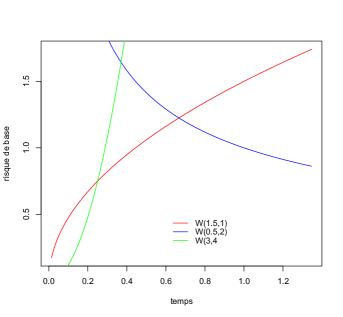
Figure 1: Plots of the baseline hazard function for different parameters of a Weibull distribution $\mathcal{W}(a,\lambda)$

We consider a rate of censoring of $20\%$ and the censoring times $C_{i}$, for $i=1,...,n$, are simulated independently from the survival times via an exponential distribution $\mathcal{E}(1/\gamma\mathbb{E}[T_{1}])$, where $\gamma=4.5$ is adjusted to the rate of censorship. The time $\tau$ of the end of the study is taken as the quantile at $90\%$ of $(T_{i}\wedge C_{i})_{i=1,...,n}$. For $i=1,...,n$, we compute the observed times $X_{i}=\min(T_{i},\tilde{C}_{i})$, where $\tilde{C}_{i}=C_{i}\wedge\tau$ and the censoring indicators $\delta_{i}=\mathds{1}_{T_{i}\leq C_{i}}$. The definition of $\tilde{C}_{i}$ ensures that there exist some $i\in\{1,...,n\}$ for which $X_{i}\geq\tau$, so that all estimators are defined on the interval $[0,\tau]$ and it prevents from certain edge effect.

Each sample $(\boldsymbol{Z_{i}},T_{i},C_{i},X_{i},\delta_{i},i=1,...,n)$ is repeated $N_{e}=100$ times.

5.2 Estimation procedures

We implement $\hat{\alpha}^{\boldsymbol{\hat{\beta}}}_{m}$ in a histogram basis defined, for $j=1,...,2^{m}$, by

$$\varphi^{m}_{j}(t)=\dfrac{1}{\sqrt{\tau}}2^{m/2}\mathds{1}_{[{(j-1)\tau/2^{m}},{j\tau/2^{m}}[}(t),$$

In this case, the cardinal of $S_{m}$ is $D_{m}=2^{m}$ and Assumption 3.5.(ii) is satisfied for $\phi=1/\tau$. We take $m=0,...,\lfloor\log(n/\log(n))/\log(2))\rfloor$, so that Assumption 3.5.(i) is fulfilled. In this basis, the estimator is being written by

$$\hat{\alpha}^{\boldsymbol{\hat{\beta}}}_{m}(t)=\sum_{j\in J_{m}}\hat{a}^{\boldsymbol{\hat{\beta}}}_{j}\varphi^{m}_{j}(t),\quad\forall t\in[0,\tau],$$ (18)

where

$$\hat{a}^{\boldsymbol{\hat{\beta}}}_{j}=\dfrac{\tau}{2^{m}}\dfrac{1}{\frac{1}{n}\displaystyle\sum_{i=1}^{n}{\mathrm{e}}^{\boldsymbol{\hat{\beta}^{T}Z_{i}}}\Big{(}\Big{(}\min\Big{(}X_{i},\frac{j\tau}{2^{m}}\Big{)}-\frac{(j-1)\tau}{2^{m}}\Big{)}\vee 0\Big{)}}\dfrac{1}{n}\displaystyle\sum_{i=1}^{n}\delta_{i}\dfrac{2^{m/2}}{\sqrt{\tau}}\mathds{1}_{\Big{[}\frac{(j-1)\tau}{2^{m}},\frac{j\tau}{2^{m}}\Big{)}}(X_{i}).$$

The final estimator $\hat{\alpha}^{\boldsymbol{\hat{\beta}}}_{\hat{m}^{\boldsymbol{\hat{\beta}}}}$ is obtained from the implementation of the selection model procedure (10), replacing in the penalty term the unknown quantity $||\alpha_{0}||_{\infty,\tau}$ by $||\hat{\alpha}^{\boldsymbol{\hat{\beta}}}_{\max(m)}||_{\infty,\tau}$, an estimator of $\alpha_{0}$ computed on the arbitrary larger space $S_{\max(m)}$.

We want to compare the performances of the estimator $\hat{\alpha}^{\boldsymbol{\hat{\beta}}}_{\hat{m}^{\boldsymbol{\hat{\beta}}}}$ to those of the usual kernel estimator with a bandwidth selected by cross-validation introduced by Ramlau-Hansen (1983b), that we have also implemented. More precisely the usual kernel estimator is defined by

$$\hat{\alpha}^{\boldsymbol{\hat{\beta}}}_{\hat{h}^{\boldsymbol{\hat{\beta}}}_{CV}}(t)=\dfrac{1}{\hat{h}^{\boldsymbol{\hat{\beta}}}_{CV}}\displaystyle\sum_{i=1}^{n}\dfrac{\delta_{i}}{\sum_{j=1}^{n}{\mathrm{e}}^{\boldsymbol{\hat{\beta}^{T}Z_{j}}}\mathds{1}_{\{X_{j}\geq X_{i}\}}}K\left(\dfrac{t-X_{i}}{\hat{h}^{\boldsymbol{\hat{\beta}}}_{CV}}\right),$$ (19)

where $K(u)=0.75(1-u^{2})\mathds{1}_{\{|u|\leq 1\}}$ is the Epanechnikov kernel and the bandwidth $\hat{h}^{\boldsymbol{\hat{\beta}}}_{CV}$ has been selected by cross-validation:

$$\hat{h}^{\boldsymbol{\hat{\beta}}}_{CV}=\underset{h}{\arg\min}\Bigg{\{}\mathbb{E}\displaystyle\int_{0}^{\tau}(\hat{\alpha}^{\boldsymbol{\hat{\beta}}}_{h}(t))^{2}\mathrm{d}t-2\sum_{i\neq j}\dfrac{1}{h}K\Big{(}\dfrac{X_{i}-X_{j}}{h}\Big{)}\dfrac{\Delta N(X_{i})}{\bar{Y}(X_{i})}\dfrac{\Delta N(X_{j})}{\bar{Y}{(X_{j})}}\Bigg{\}},$$

where $\bar{Y}=\sum_{i=1}^{n}\mathds{1}_{\{X_{i}\geq t\}}$.

Both estimators of the baseline hazard function are defined from the Lasso estimator $\boldsymbol{\hat{\beta}}$ of the regression parameter defined by (3).

The performances of these two estimators are evaluated via a random Mean Integrated Squared Error ($\operatorname{MISErand}$) adapted to the Cox model and defined by $\operatorname{MISErand}(\alpha,\boldsymbol{\hat{\beta}})=\mathbb{E}[\operatorname{ISErand}(\alpha,\boldsymbol{\hat{\beta}})]$, where the expectation is taken on $(T_{i},C_{i},\boldsymbol{Z_{i}})$ and

$$\operatorname{ISErand}(\alpha,\boldsymbol{\hat{\beta}})=\dfrac{1}{n}\displaystyle\sum_{i=1}^{n}\int_{0}^{X_{i}}(\alpha(t)-\alpha_{0}(t))^{2}{\mathrm{e}}^{\boldsymbol{\hat{\beta}^{T}Z_{i}}}\mathrm{d}t,$$ (20)

We obtain an estimation of the $\operatorname{MISErand}$ by taking the empirical mean for $N_{e}=100$ replications.

In Table 1, we give the random $\operatorname{MISE}$ of the penalized contrast estimator and of the kernel estimator with a bandwidth selected by cross-validation for different distributions of the survival times.

		$\mathcal{W}(1.5,1)$		$\mathcal{W}(0.5,2)$		$\mathcal{W}(3,4)$
$n=200$	$p=15$	0.072	0.021	0.626	1.09	5.26	8.48
	$p=200$	0.071	0.020	0.613	1.09	5.30	8.33
$n=500$	$p=22$	0.055	0.009	0.401	1.06	5.24	7.48
	$p=500$	0.059	0.008	0.402	1.06	5.25	8.10

Table 1: Random empirical MISE for the penalized contrast estimator in a histogram basis (first column for each distribution) and for the kernel estimator with a bandwidth selected by cross-validation (second column for each distribution), with a Lasso estimator of the regression parameter, for three different Weibull distributions of the survival times.

First, as expected, the random $\operatorname{MISE}$s are smaller for a large $n$ and a small $p$. Then, we observe that the penalized contrast estimator performs better than the kernel estimator for the Weibull distributions $\mathcal{W}(0.5,2)$ and $\mathcal{W}(3,4)$. Note that the random $\operatorname{MISE}$s are very high for this last distribution. This can easily be explained from the fact that the baseline hazard function associated to a $\mathcal{W}(3,4)$ has the most complicated form since it increases steeply (see Figure 1). Lastly, for the distribution $\mathcal{W}(1.5,1)$, the random $\operatorname{MISE}$s are smaller in the case of the kernel estimator with a bandwidth selected by cross-validation than in the case of the penalized contrast estimator.

6 Proofs

6.1 Technical results

In this section, we introduce some propositions and lemmas that are necessary to prove the theorems. Their proofs are postponed to Subsection 6.3.

Let us first introduce the random norm revealed from the contrast (8) and associated to the deterministic norm defined by (9), and its associated scalar product: for $\alpha$, $\alpha_{1}$ and $\alpha_{2}$ functions in $(\mathbb{L}^{2}\cap\mathbb{L}^{\infty})([0,\tau])$ and $\boldsymbol{\beta}\in\mathbb{R}^{p}$ fixed,

$$||\alpha||_{rand(\boldsymbol{\beta})}^{2} = \dfrac{1}{n}\displaystyle\sum_{i=1}^{n}\displaystyle\int_{0}^{\tau}\alpha^{2}(t){\mathrm{e}}^{\boldsymbol{\beta^{T}Z_{i}}}Y_{i}(t)\mathrm{d}t,$$ (21)

$$\langle\alpha_{1},\alpha_{2}\rangle_{rand(\boldsymbol{\beta})} = \dfrac{1}{n}\displaystyle\sum_{i=1}^{n}\displaystyle\int_{0}^{\tau}\alpha_{1}(t)\alpha_{2}(t){\mathrm{e}}^{\boldsymbol{\beta^{T}Z_{i}}}Y_{i}(t)\mathrm{d}t,$$

Subsequently, to relieve the notations, we denote $||.||_{rand}:=||.||_{rand(\boldsymbol{\beta}_{0})}$ and the same holds for the associated scalar product. We state a key relation between $\langle.,.\rangle_{rand(\boldsymbol{\beta})}$ and $C_{n}(.,\boldsymbol{\beta})$. By definition, for all $m\in\mathcal{M}_{n}$ and $\boldsymbol{\beta}\in\mathbb{R}^{p}$,

$$C_{n}(\hat{\alpha}^{\boldsymbol{\beta}}_{\hat{m}^{\boldsymbol{\beta}}},\boldsymbol{\beta})+\operatorname{pen}(\hat{m}^{\boldsymbol{\beta}})\leq C_{n}(\hat{\alpha}^{\boldsymbol{\beta}}_{m},\boldsymbol{\beta})+\operatorname{pen}(m)\leq C_{n}(\alpha^{\boldsymbol{\beta_{0}}}_{m},\boldsymbol{\beta})+\operatorname{pen}(m),$$ (22)

where $\hat{m}^{\boldsymbol{\beta}}=\arg\min_{m\in\mathcal{M}_{n}}\{C_{n}(\hat{\alpha}^{\boldsymbol{\beta}}_{m},\boldsymbol{\beta})+\operatorname{pen}(m)\}$. Now, we write that

$$C_{n}(\hat{\alpha}^{\boldsymbol{\beta}}_{\hat{m}^{\boldsymbol{\beta}}},\boldsymbol{\beta})-C_{n}(\alpha^{\boldsymbol{\beta_{0}}}_{m},\boldsymbol{\beta})$$

$$= -\dfrac{2}{n}\displaystyle\sum_{i=1}^{n}\displaystyle\int_{0}^{\tau}(\hat{\alpha}^{\boldsymbol{\beta}}_{\hat{m}^{\boldsymbol{\beta}}}-\alpha^{\boldsymbol{\beta_{0}}}_{m})(t)\mathrm{d}N_{i}(t)+\dfrac{1}{n}\displaystyle\sum_{i=1}^{n}\displaystyle\int_{0}^{\tau}(\hat{\alpha}^{\boldsymbol{\beta}}_{\hat{m}^{\boldsymbol{\beta}}}(t)^{2}-\alpha^{\boldsymbol{\beta_{0}}}_{m}(t)^{2}){\mathrm{e}}^{\boldsymbol{\beta^{T}Z_{i}}}Y_{i}(t)\mathrm{d}t.$$

Using the Doob-Meyer decomposition, we derive that

$$C_{n}(\hat{\alpha}^{\boldsymbol{\beta}}_{\hat{m}^{\boldsymbol{\beta}}},\boldsymbol{\beta})-C_{n}(\alpha^{\boldsymbol{\beta_{0}}}_{m},\boldsymbol{\beta})$$

$$= -2\langle\hat{\alpha}^{\boldsymbol{\beta}}_{\hat{m}^{\boldsymbol{\beta}}}-\alpha^{\boldsymbol{\beta_{0}}}_{m},\alpha_{0}\rangle_{rand}+||\hat{\alpha}^{\boldsymbol{\beta}}_{\hat{m}^{\boldsymbol{\beta}}}||^{2}_{rand(\boldsymbol{\beta})}-||\alpha^{\boldsymbol{\beta_{0}}}_{m}||^{2}_{rand(\boldsymbol{\beta})}-2\nu_{n}(\hat{\alpha}^{\boldsymbol{\beta}}_{\hat{m}^{\boldsymbol{\beta}}}-\alpha^{\boldsymbol{\beta_{0}}}_{m}),$$

where $\nu_{n}(\alpha)$ is defined by

$$\nu_{n}(\alpha)=\dfrac{1}{n}\displaystyle\sum_{i=1}^{n}\displaystyle\int_{0}^{\tau}\alpha(t)\mathrm{d}M_{i}(t).$$ (23)

It follows that

$$C_{n}(\hat{\alpha}^{\boldsymbol{\beta}}_{\hat{m}^{\boldsymbol{\beta}}},\boldsymbol{\beta})-C_{n}(\alpha^{\boldsymbol{\beta_{0}}}_{m},\boldsymbol{\beta}) =||\hat{\alpha}^{\boldsymbol{\beta}}_{\hat{m}^{\boldsymbol{\beta}}}-\alpha^{\boldsymbol{\beta_{0}}}_{m}||^{2}_{rand(\boldsymbol{\beta})}-2\nu_{n}(\hat{\alpha}^{\boldsymbol{\beta}}_{\hat{m}^{\boldsymbol{\beta}}}-\alpha^{\boldsymbol{\beta_{0}}}_{m})$$

$$+2\langle\hat{\alpha}^{\boldsymbol{\beta}}_{\hat{m}^{\boldsymbol{\beta}}}-\alpha^{\boldsymbol{\beta_{0}}}_{m},\alpha^{\boldsymbol{\beta_{0}}}_{m}\rangle_{rand(\boldsymbol{\beta})}-2\langle\hat{\alpha}^{\boldsymbol{\beta}}_{\hat{m}^{\boldsymbol{\beta}}}-\alpha^{\boldsymbol{\beta_{0}}}_{m},\alpha_{0}\rangle_{rand}.$$ (24)

Let us now introduce the following events :

$$\Delta_{1}=\left\{\alpha\in\mathcal{S}_{n}:\left|\dfrac{||\alpha||^{2}_{rand}}{||\alpha||^{2}_{det}}-1\right|\leq\dfrac{1}{2}\right\},\quad\mbox{and}\quad\Omega=\left\{\left|\dfrac{\hat{f}_{0}}{f_{0}}-1\right|\leq\dfrac{1}{2}\right\}$$ (25)

$$\Delta_{2}=\left\{\alpha\in\mathcal{S}_{n}:\left|\dfrac{||\alpha||^{2}_{rand(\boldsymbol{\hat{\beta}})}}{||\alpha||^{2}_{rand}}-1\right|\leq\dfrac{1}{2}\right\}.$$ (26)

On the sets $\Delta_{1}$ and $\Delta_{2}$ we have a relation between the random $||.||_{rand}$ and the deterministic $||.||_{det}$ norms and between the random norms $||.||_{rand}$ and $||.||_{rand(\boldsymbol{\hat{\beta}})}$ respectively. The following proposition state a relation between the deterministic norm (9) and the standard $\mathbb{L}^{2}$-norm:

Proposition 6.1 (Connections between the norms).

From Assumptions 2.2.(i)-(iii), we deduce the following connection between the deterministic norm and the standard $\mathbb{L}^{2}$-norm:

$$f_{0}{\mathrm{e}}^{-B|\boldsymbol{\beta_{0}}|_{1}}||\alpha||^{2}_{2}\leq||\alpha||^{2}_{det}\leq\mathbb{E}[{\mathrm{e}}^{\boldsymbol{\beta_{0}^{T}Z}}]||\alpha||^{2}_{2}\leq{\mathrm{e}}^{B|\boldsymbol{\beta_{0}}|_{1}}||\alpha||^{2}_{2}.$$

The proof of this proposition is immediate using the fact that from Assumption 2.2.(ii), we can rewrite the deterministic norm as

$$||\alpha||_{det}^{2}=\displaystyle\int_{0}^{\tau}\int_{A}\alpha^{2}(t)e^{\boldsymbol{\beta_{0}^{T}z}}\mathbb{E}[Y(t)|\boldsymbol{Z}=\boldsymbol{z}]f_{\boldsymbol{Z}}(z)\mathrm{d}z\mathrm{d}t.$$

6.1.1 Results used in the proofs of Theorem 4.1

Recall that for all $\boldsymbol{\beta}\in\mathbb{R}^{p}$,

$$\hat{\mathcal{H}}^{\boldsymbol{\beta}}_{m}=\Bigg{\{}\min\operatorname{Sp}(\boldsymbol{G^{\boldsymbol{\beta}}_{m}})\geq\max\Bigg{(}\dfrac{\hat{f}_{0}{\mathrm{e}}^{-B|\boldsymbol{\beta}_{0}|_{1}}{\mathrm{e}}^{-B|\boldsymbol{\beta}_{0}-\boldsymbol{\beta|_{1}}}}{6},\dfrac{1}{\sqrt{n}}\Bigg{)}\Bigg{\}}.$$

The following lemma ensures the existence of the estimators $\hat{\alpha}^{\boldsymbol{\hat{\beta}}}_{\hat{m}^{\boldsymbol{\hat{\beta}}}}$ on $\Delta_{1}\cap\Delta_{2}\cap\Omega$.

Lemma 6.2.

Under Assumptions 2.2.(i)-(iv), Assumptions 3.1 and Assumptions 3.5.(i)-(iii), for $n\geq 16/(f_{0}{\mathrm{e}}^{-3BR})^{2}$, the following embedding holds:

$$\Delta_{1}\cap\Delta_{2}\cap\Omega\subset\hat{\mathcal{H}}^{\boldsymbol{\hat{\beta}}}\cap\Omega,\quad\mbox{ where }\hat{\mathcal{H}}^{\boldsymbol{\hat{\beta}}}:=\underset{m\in\mathcal{M}_{n}}{\cap}\hat{\mathcal{H}}^{\boldsymbol{\hat{\beta}}}_{m}.$$

From this lemma, for all $m\in\mathcal{M}_{n}$, the matrix $\boldsymbol{G^{\hat{\beta}}_{m}}$ is invertible on $\Delta_{1}\cap\Delta_{2}\cap\Omega$, and thus the estimator of $\alpha_{0}$ is well defined. Proof 6.2 are available in Subsection 6.3.1.

The following proposition bounds the quadratic difference between $\hat{\alpha}^{\boldsymbol{\hat{\beta}}}_{\hat{m}^{\boldsymbol{\hat{\beta}}}}$ and $\alpha^{\boldsymbol{\beta_{0}}}_{m}$ for $m\in\mathcal{M}_{n}$, on the complements of

$$\aleph_{k}=\Delta_{1}\cap\Delta_{2}\cap\Omega\cap\Omega^{k}_{H},$$

where $\Omega^{k}_{H}$, (the indice $H$ is for "Huang", since the set has already been defined by Huang et al. (2013)), is defined for $k>0$ by

$$\Omega^{k}_{H}=\left\{|\boldsymbol{\hat{\beta}}-\boldsymbol{\beta_{0}}|_{1}\leq C(s)\sqrt{\dfrac{\log(pn^{k})}{n}}\right\},$$ (27)

for a constant $C(s)$ depending on the sparsity index of $\boldsymbol{\beta_{0}}$. From Proposition 3.2, $\mathbb{P}(\Omega^{k}_{H})\geq 1-cn^{-k}$ for a constant $c>0$. Now, let us state the two following propositions.

Proposition 6.3.

Under Assumptions 2.2.(i)-(iv), Assumptions 3.1 and Assumptions 3.5.(i)-(iii),

$$\mathbb{E}[||\hat{\alpha}^{\boldsymbol{\hat{\beta}}}_{\hat{m}^{\boldsymbol{\hat{\beta}}}}-\alpha^{\boldsymbol{\beta_{0}}}_{m}||^{2}_{det}\mathds{1}_{\aleph_{k}^{c}}]\leq\tilde{c}_{1}/n,$$ (28)

where $\tilde{c}_{1}$ is a constant depending on $\tau$, $\phi$, $||\alpha_{0}||_{\infty,\tau}$, $f_{0}$, $\mathbb{E}[{\mathrm{e}}^{\boldsymbol{\beta_{0}^{T}Z}}]$, $\mathbb{E}[{\mathrm{e}}^{2\boldsymbol{\beta_{0}^{T}Z}}]$, $B$, $|\boldsymbol{\beta_{0}}|_{1}$, the sparsity index $s$ of $\boldsymbol{\beta_{0}}$ and $\kappa_{b}$ a constant that comes from the Bürkholder Inequality (see Theorem 6.9).

We refer to Subsection 6.3.2 for the proof of Proposition 6.3. This propositions are directly used in the proof of Theorems 4.1 in Subsection 6.2.

Usually, in model selection (see for instance Massart (2007)), the penalty is obtained by using the so-called Talagrand’s deviation inequality for the maximum of empirical processes. In the empirical process (23), the martingales $M_{i}$, $i=1,...,n$, are unbounded, Thus, we cannot directly use the Talagrand’s inequality. We consider the following proposition proved in Comte et al. (2011). To obtain an uniform deviation of $\nu_{n}(.)$, Comte et al. (2011) have used tools from van de Geer (1995) to establish Bennett and Bernstein type inequalities and a $\mathbb{L}^{2}(det)-\mathbb{L}^{\infty}$ generic chaining type of technique (see Talagrand (2005) and Baraud (2010)).

Proposition 6.4.

Let $m,m^{\prime}\in\mathcal{M}_{n}$. Define

$$\mathcal{B}^{det}_{m,m^{\prime}}(0,1)=\{\alpha\in S_{m}+S_{m}^{\prime}:||\alpha||_{\det}\leq 1\}.$$ (29)

Under the assumptions of Theorem 4.1, there exists $\kappa>0$ such that for

$$p(m,m^{\prime})=\dfrac{\kappa}{K_{0}}(\operatorname{pen}(m)+\operatorname{pen}(m^{\prime})),$$ (30)

where the constant $K_{0}$ and $\operatorname{pen}(m)$ are defined in (16), then

$$\sum_{m^{\prime}\in\mathcal{M}_{n}}\mathbb{E}\Big{(}\Big{(}\underset{\alpha\in\mathcal{B}^{det}_{m,m^{\prime}}(0,1)}{\sup}\nu^{2}_{n}(\alpha)-p(m,m^{\prime})\Big{)}_{+}\mathds{1}_{\Delta_{1}}\Big{)}\leq\dfrac{C_{3}}{n}$$

for $n$ large enough, where $C_{3}$ is a constant depending on $f_{0}$, $\mathbb{E}[{\mathrm{e}}^{\boldsymbol{\beta_{0}^{T}Z}}]$, $B$, $|\boldsymbol{\beta_{0}}|_{1}$, $||\alpha_{0}||_{\infty,\tau}$ and the choice of the basis.

These propositions are applied to prove Theorem 4.1. We admit the proof of this proposition and refer to Comte et al. (2011) for a detailed proof of this result.

We need Proposition 6.5 to prove Theorem 4.1: the empirical centered process $\eta_{n}(\alpha,\alpha^{\boldsymbol{\beta_{0}}}_{m})$, defined by

$$\eta_{n}(\alpha,\alpha^{\boldsymbol{\beta_{0}}}_{m})=\dfrac{1}{n}\displaystyle\sum_{i=1}^{n}\Big{(}U_{i}(\alpha,\alpha^{\boldsymbol{\beta_{0}}}_{m})-\mathbb{E}[U_{i}(\alpha,\alpha^{\boldsymbol{\beta_{0}}}_{m})]\Big{)},$$

where

$$U_{i}(\alpha,\alpha^{\boldsymbol{\beta_{0}}}_{m})=\left(\displaystyle\int_{0}^{\tau}\alpha(t)\alpha^{\boldsymbol{\beta_{0}}}_{m}(t){\mathrm{e}}^{\boldsymbol{\beta_{0}^{T}Z_{i}}}Y_{i}(t)\mathrm{d}t\right)^{2}.$$

appears in the proof of Theorem 4.1, when we control the difference between the scalar products $\langle.,.\rangle_{rand}-\langle.,.\rangle_{rand(\boldsymbol{\hat{\beta}})}$ (see Subsection 6.2.1). Proposition 6.5 allows to control this process.

Proposition 6.5.

Let introduce the ball $\mathcal{B}^{det}_{n}(0,1)\subset\mathcal{S}_{n}$ defined by

$$\mathcal{B}^{det}_{n}(0,1)=\{\alpha\in\mathcal{S}_{n}:||\alpha||_{det}\leq 1\}.$$ (31)

Under Assumptions 2.2.(i)-(iv) and Assumption 3.1, we have

$$\mathbb{E}\left[\underset{\alpha\in\mathcal{B}^{det}_{n}(0,1)}{\sup}\eta_{n}(\alpha,\alpha^{\boldsymbol{\beta_{0}}}_{m})^{2}\right]\leq\dfrac{1}{n}\dfrac{\mathbb{E}[{\mathrm{e}}^{4\boldsymbol{\beta_{0}^{T}Z}}]||\alpha^{\boldsymbol{\beta_{0}}}_{m}||^{4}_{2}}{({\mathrm{e}}^{-B|\boldsymbol{\beta_{0}}|_{1}}f_{0})^{2}}.$$

Proposition 6.5 is proved in Subsection 6.3.3.

6.1.2 Technical lemmas for the proofs of Proposition LABEL:propcomp1 and 6.3

In order to prove Proposition 6.3, we need three lemmas:

Lemma 6.6.

Under Assumptions 2.2.(i)-(iv), Assumptions 3.1 and Assumptions 3.5.(i)-(iii), we have

$$\mathbb{E}[||\hat{\alpha}^{\boldsymbol{\hat{\beta}}}_{\hat{m}^{\boldsymbol{\hat{\beta}}}}||^{4}_{2}]\leq C_{b}n^{4},$$

where $C_{b}$ is constant depending on $||\alpha_{0}||_{\infty,\tau}$, $\tau$, $\mathbb{E}[{\mathrm{e}}^{\boldsymbol{\beta_{0}^{T}Z}}]$ and $\mathbb{E}[{\mathrm{e}}^{2\boldsymbol{\beta_{0}^{T}Z}}]$, $\kappa_{b}$, the constant of the Bürkholder Inequality (see Theorem 6.9) and on the choice of the basis.

Lemma 6.7.

Under Assumptions 2.2.(i)-(iv) and Assumptions 3.5.(i)-(iii), we have

$$\mathbb{P}(\Delta^{c}_{1})\leq\dfrac{C^{(\Delta_{1})}_{k}}{n^{k}},\quad\forall k\geq 1,$$

where $C^{(\Delta_{1})}_{k}$ is a constant depending on $f_{0}$, $B$ and $|\boldsymbol{\beta_{0}}|_{1}$.

Lemma 6.8.

Under Assumptions 2.2.(i)-(iv), Assumptions 3.1 and Assumption 3.3, we have for $n$ large enough,

$$\mathbb{P}(\Delta^{c}_{2})\leq\dfrac{C^{(\Delta_{2})}_{k}}{n^{k}},\quad\forall k\geq 1,$$

where the constant $C^{(\Delta_{2})}_{k}$ depends on $\tau$, $||\alpha_{0}||_{\infty,\tau}$ and $\mathbb{E}[{\mathrm{e}}^{\boldsymbol{\beta_{0}^{T}Z}}]$.

These three lemmas are required to prove Proposition 6.3. There are proved in Subsection 6.3.

6.1.3 A classical inequality: the Bürkholder Inequality

The last technical result is a Bürkholder Inequality that gives a norm relation between a martingale and its optional process. We refer to Liptser and Shiryayev (1989) p.75, for the proof of this result.

Theorem 6.9 (Bürkholder Inequality).

If $M=(M_{t},\mathcal{F}_{t})_{t\geq 0}$ is a martingale, then there are universal constants $\gamma_{b}$ and $\kappa_{b}$ (independent of $M$) such that for every $t\geq 0$

$$\gamma_{b}||\sqrt{[M]_{t}}||_{2}\leq||M_{t}||_{2}\leq\kappa_{b}||\sqrt{[M]_{t}}||_{2},$$

where $[M]_{t}$ is the quadratic variation of $M_{t}$.

This theorem is used to prove Lemma 6.6 and in the oracle inequalities of Theorem 4.1, the constants depend on $\kappa_{b}$.

6.2 Proofs of the main theorems

6.2.1 Proof of Theorem 4.1

In the following, we consider the sets $\Delta_{1}$, $\Delta_{2}$ and $\Omega$ defined by (25) and (26) and the set $\Omega^{k}_{H}$ defined by (27). For sake of simplicity in the notations, we denote $\aleph_{k}$ the intersection between the four sets: $\aleph_{k}=\Delta_{1}\cap\Delta_{2}\cap\Omega\cap\Omega^{k}_{H}$. We have the following decomposition:

$$\mathbb{E}[||\hat{\alpha}^{\boldsymbol{\hat{\beta}}}_{\hat{m}^{\boldsymbol{\hat{\beta}}}}-\alpha_{0}||^{2}_{det}]\leq 2||\alpha_{0}-\alpha^{\boldsymbol{\beta_{0}}}_{m}||^{2}_{det}+2\mathbb{E}[||\hat{\alpha}^{\boldsymbol{\hat{\beta}}}_{\hat{m}^{\boldsymbol{\hat{\beta}}}}-\alpha^{\boldsymbol{\beta_{0}}}_{m}||^{2}_{det}\mathds{1}_{\aleph_{k}}]+2\mathbb{E}[||\hat{\alpha}^{\boldsymbol{\hat{\beta}}}_{\hat{m}^{\boldsymbol{\hat{\beta}}}}-\alpha^{\boldsymbol{\beta_{0}}}_{m}||^{2}_{det}\mathds{1}_{\aleph_{k}^{c}}].$$

The first term is the usual bias term. From Proposition 6.3, we deduce that the last term is bounded by $\tilde{c}_{1}/n$. We now focus on the term $\mathbb{E}[||\hat{\alpha}^{\boldsymbol{\hat{\beta}}}_{\hat{m}^{\boldsymbol{\hat{\beta}}}}-\alpha^{\boldsymbol{\beta_{0}}}_{m}||^{2}_{det}\mathds{1}_{\aleph_{k}}]$. From Lemma 6.2, for all $m\in\mathcal{M}_{n}$, the matrices $\boldsymbol{G^{\boldsymbol{\hat{\beta}}}_{m}}$ are invertible on $\Delta_{1}\cap\Delta_{2}\cap\Omega\cap\Omega^{k}_{H}$ as soon as $n\geq 16/(f_{0}{\mathrm{e}}^{-3BR})^{2}$ and thus the estimator $\hat{\alpha}^{\boldsymbol{\hat{\beta}}}_{\hat{m}^{\boldsymbol{\hat{\beta}}}}$ of $\alpha_{0}$ is well defined. From (22) and (24), with $\boldsymbol{\beta}=\boldsymbol{\hat{\beta}}$, we have for all $m\in\mathcal{M}_{n}$,

$$||\hat{\alpha}^{\boldsymbol{\hat{\beta}}}_{\hat{m}^{\boldsymbol{\hat{\beta}}}} -\alpha^{\boldsymbol{\beta_{0}}}_{m}||^{2}_{rand(\boldsymbol{\hat{\beta}})}\leq 2\nu_{n}(\hat{\alpha}^{\boldsymbol{\hat{\beta}}}_{\hat{m}^{\boldsymbol{\hat{\beta}}}}-\alpha^{\boldsymbol{\beta_{0}}}_{m})+2\langle\hat{\alpha}^{\boldsymbol{\hat{\beta}}}_{\hat{m}^{\boldsymbol{\hat{\beta}}}}-\alpha^{\boldsymbol{\beta_{0}}}_{m},\alpha_{0}-\alpha^{\boldsymbol{\beta_{0}}}_{m}\rangle_{rand}$$

$$+\operatorname{pen}(m)-\operatorname{pen}(\hat{m}^{\boldsymbol{\hat{\beta}}})+2\langle\hat{\alpha}^{\boldsymbol{\hat{\beta}}}_{\hat{m}^{\boldsymbol{\hat{\beta}}}}-\alpha^{\boldsymbol{\beta_{0}}}_{m},\alpha^{\boldsymbol{\beta_{0}}}_{m}\rangle_{rand}-2\langle\hat{\alpha}^{\boldsymbol{\hat{\beta}}}_{\hat{m}^{\boldsymbol{\hat{\beta}}}}-\alpha^{\boldsymbol{\beta_{0}}}_{m},\alpha^{\boldsymbol{\beta_{0}}}_{m}\rangle_{rand(\boldsymbol{\hat{\beta}})},$$

where the empirical process $\nu_{n}(.)$ is defined by Equation (23) and the random norm by (21). For $\mathcal{B}^{det}_{m,m^{\prime}}(0,1)$ defined by (29), using the classical inequality $2xy\leq\leavevmode\nobreak\ bx^{2}+y^{2}/b$ with $b>0$, we obtain

$$||\hat{\alpha}^{\boldsymbol{\hat{\beta}}}_{\hat{m}^{\boldsymbol{\hat{\beta}}}}-\alpha^{\boldsymbol{\beta_{0}}}_{m}||^{2}_{rand(\boldsymbol{\hat{\beta}})} \leq\dfrac{1}{16}||\hat{\alpha}^{\boldsymbol{\hat{\beta}}}_{\hat{m}^{\boldsymbol{\hat{\beta}}}}-\alpha^{\boldsymbol{\beta_{0}}}_{m}||^{2}_{rand}+16||\alpha_{0}-\alpha^{\boldsymbol{\beta_{0}}}_{m}||^{2}_{rand}+\operatorname{pen}(m)-\operatorname{pen}(\hat{m}^{\boldsymbol{\hat{\beta}}})$$

$$+\dfrac{1}{16}||\hat{\alpha}^{\boldsymbol{\hat{\beta}}}_{\hat{m}^{\boldsymbol{\hat{\beta}}}}-\alpha^{\boldsymbol{\beta_{0}}}_{m}||^{2}_{det}+16\underset{\alpha\in\mathcal{B}^{det}_{m,\hat{m}^{\boldsymbol{\hat{\beta}}}}(0,1)}{\sup}\nu^{2}_{n}(\alpha)$$

$$+2\Big{(}\langle\hat{\alpha}^{\boldsymbol{\hat{\beta}}}_{\hat{m}^{\boldsymbol{\hat{\beta}}}}-\alpha^{\boldsymbol{\beta_{0}}}_{m},\alpha^{\boldsymbol{\beta_{0}}}_{m}\rangle_{rand}-\langle\hat{\alpha}^{\boldsymbol{\hat{\beta}}}_{\hat{m}^{\boldsymbol{\hat{\beta}}}}-\alpha^{\boldsymbol{\beta_{0}}}_{m},\alpha^{\boldsymbol{\beta_{0}}}_{m}\rangle_{rand(\boldsymbol{\hat{\beta}})}\Big{)}.$$

Consequently, using the relations between the random norms $||.||_{rand(\boldsymbol{\boldsymbol{\hat{\beta}}})}$ and $||.||_{rand}$ and between the random norm $||.||_{rand}$ and the deterministic norm $||.||_{det}$ on $\aleph_{k}$, we obtain

$$\dfrac{1}{4}||\hat{\alpha}^{\boldsymbol{\hat{\beta}}}_{\hat{m}^{\boldsymbol{\hat{\beta}}}}-\alpha^{\boldsymbol{\beta_{0}}}_{m}||^{2}_{det} \leq\dfrac{3}{32}||\hat{\alpha}^{\boldsymbol{\hat{\beta}}}_{\hat{m}^{\boldsymbol{\hat{\beta}}}}-\alpha^{\boldsymbol{\beta_{0}}}_{m}||^{2}_{det}+16||\alpha_{0}-\alpha^{\boldsymbol{\beta_{0}}}_{m}||^{2}_{rand}+\operatorname{pen}(m)-\operatorname{pen}(\hat{m}^{\boldsymbol{\hat{\beta}}})$$

$$\hskip 19.91684pt+\dfrac{1}{16}||\hat{\alpha}^{\boldsymbol{\hat{\beta}}}_{\hat{m}^{\boldsymbol{\hat{\beta}}}}-\alpha^{\boldsymbol{\beta_{0}}}_{m}||^{2}_{det}+16\underset{\alpha\in\mathcal{B}^{det}_{m,\hat{m}^{\boldsymbol{\hat{\beta}}}}(0,1)}{\sup}\nu^{2}_{n}(\alpha)$$

$$\hskip 19.91684pt+2\Big{(}\langle\hat{\alpha}^{\boldsymbol{\hat{\beta}}}_{\hat{m}^{\boldsymbol{\hat{\beta}}}}-\alpha^{\boldsymbol{\beta_{0}}}_{m},\alpha^{\boldsymbol{\beta_{0}}}_{m}\rangle_{rand}-\langle\hat{\alpha}^{\boldsymbol{\hat{\beta}}}_{\hat{m}^{\boldsymbol{\hat{\beta}}}}-\alpha^{\boldsymbol{\beta_{0}}}_{m},\alpha^{\boldsymbol{\beta_{0}}}_{m}\rangle_{rand(\boldsymbol{\hat{\beta}})}\Big{)},$$

also be rewritten for $p(m,m^{\prime})$ defined by (30) for all $m^{\prime}\in\mathcal{M}_{n}$, as

$$\dfrac{3}{32}\mathbb{E}\Big{[}||\hat{\alpha}^{\boldsymbol{\hat{\beta}}}_{\hat{m}^{\boldsymbol{\hat{\beta}}}}-\alpha^{\boldsymbol{\beta_{0}}}_{m}||^{2}_{det}\mathds{1}_{\aleph_{k}}\Big{]}\leq 16||\alpha_{0}-\alpha^{\boldsymbol{\beta_{0}}}_{m}||^{2}_{det}+16p(m,\hat{m}^{\boldsymbol{\hat{\beta}}})$$

$$+\operatorname{pen}(m)-\operatorname{pen}(\hat{m}^{\boldsymbol{\hat{\beta}}})+16\displaystyle\sum_{m^{\prime}\in\mathcal{M}_{n}}\mathbb{E}\Bigg{(}\Bigg{(}\underset{\alpha\in\mathcal{B}^{det}_{m,m^{\prime}}(0,1)}{\sup}\nu^{2}_{n}(\alpha)-p(m,m^{\prime})\Bigg{)}_{+}\mathds{1}_{\aleph_{k}}\Bigg{)}$$

$$+2\mathbb{E}\Big{[}\Big{(}\langle\hat{\alpha}^{\boldsymbol{\hat{\beta}}}_{\hat{m}^{\boldsymbol{\hat{\beta}}}}-\alpha^{\boldsymbol{\beta_{0}}}_{m},\alpha^{\boldsymbol{\beta_{0}}}_{m}\rangle_{rand}-\langle\hat{\alpha}^{\boldsymbol{\hat{\beta}}}_{\hat{m}^{\boldsymbol{\hat{\beta}}}}-\alpha^{\boldsymbol{\beta_{0}}}_{m},\alpha^{\boldsymbol{\beta_{0}}}_{m}\rangle_{rand(\boldsymbol{\hat{\beta}})}\Big{)}\mathds{1}_{\aleph_{k}}\Big{]}.$$

We fix $K_{0}\geq 16\kappa$ such that $16p(m,m^{\prime})\leq\operatorname{pen}(m)+\operatorname{pen}(m^{\prime})$, for all $m,m^{\prime}$ in $\mathcal{M}_{n}$, so that

$$\dfrac{3}{32}\mathbb{E}\Big{[}||\hat{\alpha}^{\boldsymbol{\hat{\beta}}}_{\hat{m}^{\boldsymbol{\hat{\beta}}}}-\alpha^{\boldsymbol{\beta_{0}}}_{m}||^{2}_{det} \mathds{1}_{\aleph_{k}}\Big{]}\leq 16||\alpha_{0}-\alpha^{\boldsymbol{\beta_{0}}}_{m}||^{2}_{det}+2\operatorname{pen}(m)$$

$$+16\displaystyle\sum_{m^{\prime}\in\mathcal{M}_{n}}\mathbb{E}\Big{(}\Big{(}\underset{\alpha\in\mathcal{B}^{det}_{m,m^{\prime}}(0,1)}{\sup}\nu^{2}_{n}(\alpha)-p(m,m^{\prime})\Big{)}_{+}\mathds{1}_{\aleph_{k}}\Big{)}$$

$$+2\mathbb{E}\Big{[}\Big{(}\langle\hat{\alpha}^{\boldsymbol{\hat{\beta}}}_{\hat{m}^{\boldsymbol{\hat{\beta}}}}-\alpha^{\boldsymbol{\beta_{0}}}_{m},\alpha^{\boldsymbol{\beta_{0}}}_{m}\rangle_{rand}-\langle\hat{\alpha}^{\boldsymbol{\hat{\beta}}}_{\hat{m}^{\boldsymbol{\hat{\beta}}}}-\alpha^{\boldsymbol{\beta_{0}}}_{m},\alpha^{\boldsymbol{\beta_{0}}}_{m}\rangle_{rand(\boldsymbol{\hat{\beta}})}\Big{)}\mathds{1}_{\aleph_{k}}\Big{]},$$

that is

$$\dfrac{3}{32}\mathbb{E}[||\hat{\alpha}^{\boldsymbol{\hat{\beta}}}_{\hat{m}^{\boldsymbol{\hat{\beta}}}}-\alpha^{\boldsymbol{\beta_{0}}}_{m}||^{2}_{det}\mathds{1}_{\aleph_{k}}]\leq 16||\alpha_{0}-\alpha^{\boldsymbol{\beta_{0}}}_{m}||^{2}_{det}+2\operatorname{pen}(m)+A(m)+\mathbb{E}[B(m,\hat{m}^{\boldsymbol{\hat{\beta}}})\mathds{1}_{\aleph_{k}}]$$ (32)

where

$$A(m) =16\displaystyle\sum_{m^{\prime}\in\mathcal{M}_{n}}\mathbb{E}\Bigg{(}\Bigg{(}\underset{\alpha\in\mathcal{B}^{det}_{m,m^{\prime}}(0,1)}{\sup}\nu^{2}_{n}(\alpha)-p(m,m^{\prime})\Bigg{)}_{+}\mathds{1}_{\aleph_{k}}\Bigg{)},$$ (33)

$$B(m,\hat{m}^{\boldsymbol{\hat{\beta}}}) =2\Big{(}\langle\hat{\alpha}^{\boldsymbol{\hat{\beta}}}_{\hat{m}^{\boldsymbol{\hat{\beta}}}}-\alpha^{\boldsymbol{\beta_{0}}}_{m},\alpha^{\boldsymbol{\beta_{0}}}_{m}\rangle_{rand}-\langle\hat{\alpha}^{\boldsymbol{\hat{\beta}}}_{\hat{m}^{\boldsymbol{\hat{\beta}}}}-\alpha^{\boldsymbol{\beta_{0}}}_{m},\alpha^{\boldsymbol{\beta_{0}}}_{m}\rangle_{rand(\boldsymbol{\hat{\beta}})}\Big{)}.$$ (34)

It remains to study the terms $A(m)$ and $B(m,\hat{m}^{\boldsymbol{\hat{\beta}}})$.

Study of (33).

According to Proposition 6.4, for $n$ large enough

$$\sum_{m^{\prime}\in\mathcal{M}_{n}}\mathbb{E}\Bigg{(}\Bigg{(}\underset{\alpha\in\mathcal{B}^{det}_{m,m^{\prime}}(0,1)}{\sup}\nu^{2}_{n}(\alpha)-p(m,m^{\prime})\Bigg{)}_{+}\mathds{1}_{\aleph_{k}}\Bigg{)}\leq\dfrac{C_{3}}{n},$$

where $p(m,m^{\prime})$ is defined by (30) and $C_{3}$ is a constant depending on $f_{0}$, $|\boldsymbol{\beta_{0}}|_{1}$, $B$, $\mathbb{E}[{\mathrm{e}}^{\boldsymbol{\beta_{0}^{T}Z}}]$, $||\alpha_{0}||_{\infty,\tau}$ and the choice of the basis. Hence, for $C^{\prime}_{3}=16C_{3}$, we conclude that

$$A(m)\leq\dfrac{C^{\prime}_{3}}{n}.$$ (35)

Study of (34).

Using again the classical inequality $2xy\leq bx^{2}+y^{2}/b$ with $b>0$, we obtain

$$\langle \hat{\alpha}^{\boldsymbol{\hat{\beta}}}_{\hat{m}^{\boldsymbol{\hat{\beta}}}}-\alpha^{\boldsymbol{\beta_{0}}}_{m},\alpha^{\boldsymbol{\beta_{0}}}_{m}\rangle_{rand}-\langle\hat{\alpha}^{\boldsymbol{\hat{\beta}}}_{\hat{m}^{\boldsymbol{\hat{\beta}}}}-\alpha^{\boldsymbol{\beta_{0}}}_{m},\alpha^{\boldsymbol{\beta_{0}}}_{m}\rangle_{rand(\boldsymbol{\hat{\beta}})}\leq\dfrac{1}{32}||\hat{\alpha}^{\boldsymbol{\hat{\beta}}}_{\hat{m}^{\boldsymbol{\hat{\beta}}}}-\alpha^{\boldsymbol{\beta_{0}}}_{m}||^{2}_{det}$$

$$+32\underset{\alpha\in\mathcal{B}^{det}_{m,\hat{m}^{\hat{\beta}}}(0,1)}{\sup}\Big{(}\dfrac{1}{n}\displaystyle\sum_{i=1}^{n}\displaystyle\int_{0}^{\tau}\alpha(t)\alpha^{\boldsymbol{\beta_{0}}}_{m}(t)({\mathrm{e}}^{\boldsymbol{\beta_{0}^{T}Z_{i}}}-{\mathrm{e}}^{\boldsymbol{\hat{\beta}^{T}Z_{i}}})Y_{i}(t)\mathrm{d}t\Big{)}^{2}.$$ (36)

Now, from Assumption 3.5.(iii) and by definition (31) of $\mathcal{B}^{det}_{n}(0,1)$, we write that

$$\underset{\alpha\in\mathcal{B}^{det}_{m,\hat{m}^{\hat{\beta}}}(0,1)}{\sup}\Bigg{(}\dfrac{1}{n}\displaystyle\sum_{i=1}^{n}\displaystyle\int_{0}^{\tau}\alpha(t)\alpha^{\boldsymbol{\beta_{0}}}_{m}(t)({\mathrm{e}}^{\boldsymbol{\beta_{0}^{T}Z_{i}}}-{\mathrm{e}}^{\boldsymbol{\hat{\beta}^{T}Z_{i}}})Y_{i}(t)\mathrm{d}t\Bigg{)}^{2}$$

is less than

$$\underset{\alpha\in\mathcal{B}^{det}_{n}(0,1)}{\sup}\Bigg{(}\dfrac{1}{n}\displaystyle\sum_{i=1}^{n}\displaystyle\int_{0}^{\tau}\alpha(t)\alpha^{\boldsymbol{\beta_{0}}}_{m}(t){\mathrm{e}}^{\boldsymbol{\beta_{0}^{T}Z_{i}}}(1-{\mathrm{e}}^{\boldsymbol{\hat{\beta}^{T}Z_{i}}-\boldsymbol{\beta_{0}^{T}Z_{i}}})Y_{i}(t)\mathrm{d}t\Bigg{)}^{2}.$$

We have

$$\Bigg{|}\dfrac{1}{n}\displaystyle\sum_{i=1}^{n} \displaystyle\int_{0}^{\tau}\alpha(t)\alpha^{\boldsymbol{\beta_{0}}}_{m}(t){\mathrm{e}}^{\boldsymbol{\beta_{0}^{T}Z_{i}}}(1-{\mathrm{e}}^{\boldsymbol{\hat{\beta}^{T}Z_{i}}-\boldsymbol{\beta_{0}^{T}Z_{i}}})Y_{i}(t)\mathrm{d}t\Bigg{|}$$

$$\leq\dfrac{1}{n}\displaystyle\sum_{i=1}^{n}\Big{|}1-{\mathrm{e}}^{\boldsymbol{\hat{\beta}^{T}Z_{i}}-\boldsymbol{\beta_{0}^{T}Z_{i}}}\Big{|}\Bigg{|}\displaystyle\int_{0}^{\tau}\alpha(t)\alpha^{\boldsymbol{\beta_{0}}}_{m}(t){\mathrm{e}}^{\boldsymbol{\beta_{0}^{T}Z_{i}}}Y_{i}(t)\mathrm{d}t\Bigg{|}.$$

Using the fact that $|{\mathrm{e}}^{x}-{\mathrm{e}}^{y}|\leq|x-y|{\mathrm{e}}^{x\vee y}$ for all $(x,y)\in\mathbb{R}^{2}$ and applying Assumptions 2.2.(i) and Assumptions 3.1, we obtain that

$$\Bigg{|}\dfrac{1}{n}\displaystyle\sum_{i=1}^{n} \displaystyle\int_{0}^{\tau}\alpha(t)\alpha^{\boldsymbol{\beta_{0}}}_{m}(t){\mathrm{e}}^{\boldsymbol{\beta_{0}^{T}Z_{i}}}(1-{\mathrm{e}}^{\boldsymbol{\hat{\beta}^{T}Z_{i}}-\boldsymbol{\beta_{0}^{T}Z_{i}}})Y_{i}(t)\mathrm{d}t\Bigg{|}$$

$$\leq\dfrac{1}{n}\displaystyle\sum_{i=1}^{n}|\boldsymbol{\hat{\beta}^{T}Z_{i}}-\boldsymbol{\beta_{0}^{T}Z_{i}}|{\mathrm{e}}^{|\boldsymbol{\hat{\beta}^{T}Z_{i}}-\boldsymbol{\beta_{0}^{T}Z_{i}}|}\Bigg{|}\displaystyle\int_{0}^{\tau}\alpha(t)\alpha^{\boldsymbol{\beta_{0}}}_{m}(t){\mathrm{e}}^{\boldsymbol{\beta_{0}^{T}Z_{i}}}Y_{i}(t)\mathrm{d}t\Bigg{|}$$

$$\leq B{\mathrm{e}}^{2BR}|\boldsymbol{\hat{\beta}}-\boldsymbol{\beta_{0}}|_{1}\Bigg{|}\displaystyle\int_{0}^{\tau}\alpha(t)\alpha^{\boldsymbol{\beta_{0}}}_{m}(t){\mathrm{e}}^{\boldsymbol{\beta_{0}^{T}Z_{i}}}Y_{i}(t)\mathrm{d}t\Bigg{|}.$$

Now, write

$$\underset{\alpha\in\mathcal{B}^{det}_{n}(0,1)}{\sup}\Bigg{(}\dfrac{1}{n}\displaystyle\sum_{i=1}^{n}\displaystyle\int_{0}^{\tau}\alpha(t)\alpha^{\boldsymbol{\beta_{0}}}_{m}(t){\mathrm{e}}^{\boldsymbol{\beta_{0}^{T}Z_{i}}}(1-{\mathrm{e}}^{\boldsymbol{\hat{\beta}^{T}Z_{i}}-\boldsymbol{\beta_{0}^{T}Z_{i}}})Y_{i}(t)\mathrm{d}t\Bigg{)}^{2}$$

$$\leq B^{2}{\mathrm{e}}^{4BR}|\boldsymbol{\hat{\beta}}-\boldsymbol{\beta_{0}}|^{2}_{1}\underset{\alpha\in\mathcal{B}^{det}_{n}(0,1)}{\sup}\dfrac{1}{n}\displaystyle\sum_{i=1}^{n}\Bigg{(}\displaystyle\int_{0}^{\tau}\alpha(t)\alpha^{\boldsymbol{\beta_{0}}}_{m}(t){\mathrm{e}}^{\boldsymbol{\beta_{0}^{T}Z_{i}}}Y_{i}(t)\mathrm{d}t\Bigg{)}^{2}$$

$$\leq B^{2}{\mathrm{e}}^{4BR}|\boldsymbol{\hat{\beta}}-\boldsymbol{\beta_{0}}|^{2}_{1}\underset{\alpha\in\mathcal{B}^{det}_{n}(0,1)}{\sup}\{\eta_{n}(\alpha,\alpha^{\boldsymbol{\beta_{0}}}_{m})+D_{n}(\alpha,\alpha^{\boldsymbol{\beta_{0}}}_{m})\}$$ (37)

where $\eta_{n}(\alpha,\alpha^{\boldsymbol{\beta_{0}}}_{m})$ is defined by

$$\eta_{n}(\alpha,\alpha^{\boldsymbol{\beta_{0}}}_{m})=\dfrac{1}{n}\displaystyle\sum_{i=1}^{n}\Bigg{[}\Bigg{(}\displaystyle\int_{0}^{\tau}\alpha(t)\alpha^{\boldsymbol{\beta_{0}}}_{m}(t){\mathrm{e}}^{\boldsymbol{\beta_{0}^{T}Z_{i}}}Y_{i}(t)\mathrm{d}t\Bigg{)}^{2}-\mathbb{E}\Bigg{[}\Bigg{(}\displaystyle\int_{0}^{\tau}\alpha(t)\alpha^{\boldsymbol{\beta_{0}}}_{m}(t){\mathrm{e}}^{\boldsymbol{\beta_{0}^{T}Z_{i}}}Y_{i}(t)\mathrm{d}t\Bigg{)}^{2}\Bigg{]}\Bigg{]},$$

and

$$D_{n}(\alpha,\alpha^{\boldsymbol{\beta_{0}}}_{m})=\mathbb{E}\left[\left(\displaystyle\int_{0}^{\tau}\alpha(t)\alpha^{\boldsymbol{\beta_{0}}}_{m}(t){\mathrm{e}}^{\boldsymbol{\beta_{0}^{T}Z}}Y(t)\mathrm{d}t\right)^{2}\right].$$

We first claim that the term $\sup_{\alpha\in\mathcal{B}^{det}_{n}(0,1)}\{D_{n}(\alpha,\alpha^{\boldsymbol{\beta_{0}}}_{m})\}$ is bounded, by using that from the Cauchy-Schwarz Inequality,

$$\underset{\alpha\in\mathcal{B}^{det}_{n}(0,1)}{\sup}\mathbb{E}\left[\left(\displaystyle\int_{0}^{\tau}\alpha(t)\alpha^{\boldsymbol{\beta_{0}}}_{m}(t){\mathrm{e}}^{\boldsymbol{\beta_{0}^{T}Z}}Y(t)\mathrm{d}t\right)^{2}\right]\leq||\alpha^{\boldsymbol{\beta_{0}}}_{m}||^{2}_{det}.$$

Thus, gathering bounds (36) and (37, we obtain that

$$B(m,\hat{m}^{\boldsymbol{\hat{\beta}}})\leq\dfrac{1}{16}||\hat{\alpha}^{\boldsymbol{\hat{\beta}}}_{\hat{m}^{\boldsymbol{\hat{\beta}}}}-\alpha^{\boldsymbol{\beta_{0}}}_{m}||^{2}_{det}+64\Bigg{[}B^{2}{\mathrm{e}}^{4BR}|\boldsymbol{\hat{\beta}}-\boldsymbol{\beta_{0}}|^{2}_{1}\Big{(}\underset{\alpha\in\mathcal{B}^{det}_{n}(0,1)}{\sup}\{\eta_{n}(\alpha,\alpha^{\boldsymbol{\beta_{0}}}_{m})\}+||\alpha^{\boldsymbol{\beta_{0}}}_{m}||^{2}_{det}\Big{)}\Bigg{]}.$$

So, taking the expectation and applying Proposition 6.5 to control

$$\mathbb{E}[{\sup}_{\alpha\in\mathcal{B}^{det}_{n}(0,1)}(\eta_{n}(\alpha,\alpha^{\boldsymbol{\beta_{0}}}_{m}))^{2}],$$

we get

$$\mathbb{E}[B(m,\hat{m}^{\boldsymbol{\hat{\beta}}})\mathds{1}_{\aleph_{k}}]\leq\dfrac{1}{16}\mathbb{E}[||\hat{\alpha}^{\boldsymbol{\hat{\beta}}}_{\hat{m}^{\boldsymbol{\hat{\beta}}}}-\alpha^{\boldsymbol{\beta_{0}}}_{m}||^{2}_{det}\mathds{1}_{\aleph_{k}}]$$

$$+ 64B^{2}{\mathrm{e}}^{4BR}\Bigg{\{}\mathbb{E}^{1/2}[|\boldsymbol{\hat{\beta}}-\boldsymbol{\beta_{0}}|^{4}_{1}\mathds{1}_{\aleph_{k}}]\mathbb{E}^{1/2}\Bigg{[}\underset{\alpha\in\mathcal{B}^{det}_{n}(0,1)}{\sup}\{\eta^{2}_{n}(\alpha,\alpha^{\boldsymbol{\beta_{0}}}_{m})\}\Bigg{]}+||\alpha^{\boldsymbol{\beta_{0}}}_{m}||^{2}_{det}\mathbb{E}[|\boldsymbol{\hat{\beta}}-\boldsymbol{\beta_{0}}|^{2}_{1}\mathds{1}_{\aleph_{k}}]\Bigg{\}}.$$ (38)

Finally, combining (32), (35) and (38) we conclude that

$$\dfrac{1}{16}\mathbb{E}[||\hat{\alpha}^{\boldsymbol{\hat{\beta}}}_{\hat{m}^{\boldsymbol{\hat{\beta}}}}-\alpha^{\boldsymbol{\beta_{0}}}_{m}||^{2}_{det}\mathds{1}_{\aleph_{k}}] \leq 16||\alpha_{0}-\alpha^{\boldsymbol{\beta_{0}}}_{m}||^{2}_{det}+2\operatorname{pen}(m)+\dfrac{C^{\prime}_{3}}{n}$$

$$+64B^{2}{\mathrm{e}}^{4BR}||\alpha^{\boldsymbol{\beta_{0}}}_{m}||^{2}_{det}\mathbb{E}[|\boldsymbol{\hat{\beta}}-\boldsymbol{\beta_{0}}|^{2}_{1}\mathds{1}_{\aleph_{k}}]$$

$$+64B^{2}{\mathrm{e}}^{4BR}\mathbb{E}^{1/2}[|\boldsymbol{\hat{\beta}}-\boldsymbol{\beta_{0}}|^{4}_{1}\mathds{1}_{\aleph_{k}}]\dfrac{\mathbb{E}^{1/2}[{\mathrm{e}}^{4\boldsymbol{\beta_{0}^{T}Z}}]||\alpha^{\boldsymbol{\beta_{0}}}_{m}||^{2}_{2}}{{\mathrm{e}}^{-B|\boldsymbol{\beta_{0}}|_{1}}f_{0}}\dfrac{1}{\sqrt{n}}.$$

On $\Omega\cap\Omega^{k}_{H}$, using that, from definition (15) and Proposition 6.1, $||\alpha^{\boldsymbol{\beta_{0}}}_{m}||^{2}_{det}\leq 2||\alpha_{0}||_{det}\leq\mathbb{E}[{\mathrm{e}}^{\boldsymbol{\beta_{0}}^{T}Z}]\tau||\alpha_{0}||_{\infty,\tau}$, we have

$$64B^{2}{\mathrm{e}}^{4BR}||\alpha^{\boldsymbol{\beta_{0}}}_{m}||^{2}_{det}\mathbb{E}[|\boldsymbol{\hat{\beta}}-\boldsymbol{\beta_{0}}|^{2}_{1}\mathds{1}_{\aleph_{k}}]\leq C(s,B,R,\mathbb{E}[{\mathrm{e}}^{\boldsymbol{\beta_{0}^{T}Z}}],||\alpha_{0}||_{\infty,\tau},\tau)\dfrac{\log(pn^{k})}{n},$$

and that

$$64B^{2}{\mathrm{e}}^{4BR} \mathbb{E}^{1/2}[|\boldsymbol{\hat{\beta}}-\boldsymbol{\beta_{0}}|^{4}_{1}\mathds{1}_{\aleph_{k}}]\dfrac{\mathbb{E}^{1/2}[{\mathrm{e}}^{4\boldsymbol{\beta_{0}^{T}Z}}]||\alpha^{\boldsymbol{\beta_{0}}}_{m}||^{2}_{2}}{{\mathrm{e}}^{-B|\boldsymbol{\beta_{0}}|_{1}}f_{0}}\dfrac{1}{\sqrt{n}}$$

$$\leq\tilde{C}(s,B,|\boldsymbol{\beta_{0}}|_{1},R,\mathbb{E}[{\mathrm{e}}^{\boldsymbol{\beta_{0}^{T}Z}}],\mathbb{E}[{\mathrm{e}}^{4\boldsymbol{\beta_{0}^{T}Z}}],||\alpha_{0}||_{\infty,\tau},\tau,f_{0})\dfrac{\log(pn^{k})}{n\sqrt{n}},$$

where $s$ is the sparsiy index of $\boldsymbol{\beta_{0}}$ and

$$C(s,B,R,\mathbb{E}[{\mathrm{e}}^{\boldsymbol{\beta_{0}^{T}Z}}],||\alpha_{0}||_{\infty,\tau},\tau)\quad\text{and}\quad\tilde{C}(s,B,|\boldsymbol{\beta_{0}}|_{1},R,\mathbb{E}[{\mathrm{e}}^{\boldsymbol{\beta_{0}^{T}Z}}],\mathbb{E}[{\mathrm{e}}^{4\boldsymbol{\beta_{0}^{T}Z}}],||\alpha_{0}||_{\infty,\tau},\tau,f_{0})$$

are constants depending on the elements in brackets. Combining the previous bounds with Proposition 6.3, we conclude that Theorem 4.1 is proved since

$$\mathbb{E}[||\hat{\alpha}^{\boldsymbol{\hat{\beta}}}_{\hat{m}^{\boldsymbol{\hat{\beta}}}}-\alpha^{\boldsymbol{\beta_{0}}}_{m}||^{2}_{det}]\leq\kappa_{0}\underset{m\in\mathcal{M}_{n}}{\inf}\{||\alpha_{0}-\alpha^{\boldsymbol{\beta_{0}}}_{m}||^{2}_{det}+2\operatorname{pen}(m)\}+\dfrac{C_{1}}{n}+C_{2}\dfrac{\log(pn)}{n},$$

where $C_{1}$ and $C_{2}$ are constants depending on the sparsity index $s$ of $\boldsymbol{\beta_{0}}$, $B$, $|\boldsymbol{\beta_{0}}|_{1}$, $\mathbb{E}[{\mathrm{e}}^{\boldsymbol{\beta_{0}^{T}Z}}]$, $\mathbb{E}[{\mathrm{e}}^{4\boldsymbol{\beta_{0}^{T}Z}}]$,$||\alpha_{0}||_{\infty,\tau}$, $\tau$, ${f}_{0}$.

∎

6.2.2 Proof of Corollary 4.2

From Proposition 6.1 and the proof of Corollary 1 in Comte et al. (2011), we deduce that

$$\mathbb{E}[||\hat{\alpha}^{\boldsymbol{\hat{\beta}}}_{\hat{m}^{\boldsymbol{\hat{\beta}}}}-\alpha_{0}||^{2}_{2}] \leq\dfrac{{\mathrm{e}}^{B|\boldsymbol{\beta_{0}}|_{1}}}{f_{0}}\mathbb{E}[||\hat{\alpha}^{\boldsymbol{\hat{\beta}}}_{\hat{m}^{\boldsymbol{\hat{\beta}}}}-\alpha_{0}||^{2}_{det}]\leq\tilde{C}_{1}\underset{m\in\mathcal{M}_{n}}{\inf}\Bigg{\{}D_{m}^{-2\gamma}+\dfrac{D_{m}}{n}\Bigg{\}}+\tilde{C}_{2}(s)\dfrac{\log(np)}{n},$$

and since

$$\underset{m\in\mathcal{M}_{n}}{\inf}\Bigg{\{}D_{m}^{-2\gamma}+\dfrac{D_{m}}{n}\Bigg{\}}=n^{-\frac{2\gamma}{2\gamma+1}},$$

we finally get the corollary. ∎

6.3 Proofs of the technical propositions and lemmas

6.3.1 Proof of Lemma 6.2

Let $m\in\mathcal{M}_{n}$ be fixed and let $v$ be an eigenvalue of $\boldsymbol{G^{\boldsymbol{\hat{\beta}}}_{m}}$. There exists $\boldsymbol{A_{m}}\neq 0$ with coefficients $(a_{j})_{j}$ such that $\boldsymbol{G^{\boldsymbol{\hat{\beta}}}_{m}}\boldsymbol{A_{m}}=v\boldsymbol{A_{m}}$ and thus $\boldsymbol{A^{T}_{m}}\boldsymbol{G^{\boldsymbol{\hat{\beta}}}_{m}}\boldsymbol{A_{m}}=v\boldsymbol{A^{T}_{m}}\boldsymbol{A_{m}}$. Now, take $h:=\sum_{j}a_{j}\varphi_{j}\in S_{m}$. We have $||h||^{2}_{rand(\boldsymbol{\hat{\beta}})}=\boldsymbol{A^{T}_{m}}\boldsymbol{G^{\boldsymbol{\hat{\beta}}}_{m}}\boldsymbol{A^{T}_{m}}$ and $||h||^{2}_{2}=\boldsymbol{A^{T}_{m}A_{m}}$. Thus, on $\Delta_{1}\cap\Delta_{2}$ defined in (25) and (26) and from Proposition 6.1:

$$\boldsymbol{A^{T}_{m}\boldsymbol{G^{\boldsymbol{\hat{\beta}}}_{m}}A^{T}_{m}}=||h||^{2}_{rand(\boldsymbol{\hat{\beta}})}\geq\dfrac{1}{2}||h||^{2}_{rand}\geq\dfrac{1}{4}||h||^{2}_{det}\geq\dfrac{1}{4}f_{0}{\mathrm{e}}^{-B|\boldsymbol{\beta_{0}}|_{1}}||h||^{2}_{2}.$$

Therefore, on $\Delta_{1}\cap\Delta_{2}$, for all $m\in\mathcal{M}_{n}$, we have $\min\operatorname{Sp}(\boldsymbol{G^{\boldsymbol{\hat{\beta}}}_{m}})\geq f_{0}{\mathrm{e}}^{-3BR}/4$. Moreover, on $\Omega$, we have $f_{0}\geq 2\hat{f}_{0}/3$ and $\max(\hat{f}_{0}{\mathrm{e}}^{-3BR}/6,n^{-1/2})=\hat{f}_{0}{\mathrm{e}}^{-3BR}/6$ for $n\geq 36/(\hat{f}_{0}{\mathrm{e}}^{-3BR})^{2}$, which is equivalent on $\Omega$ to choose $n\geq 16/(f_{0}{\mathrm{e}}^{-3BR})^{2}$. ∎

6.3.2 Proof of Proposition 6.3

We have the following decomposition :

$$\mathbb{E}[||\hat{\alpha}^{\boldsymbol{\hat{\beta}}}_{\hat{m}^{\boldsymbol{\hat{\beta}}}}-\alpha^{\boldsymbol{\beta_{0}}}_{m}||^{2}_{det}\mathds{1}_{\aleph_{k}^{c}}]\leq \mathbb{E}[||\hat{\alpha}^{\boldsymbol{\hat{\beta}}}_{\hat{m}^{\boldsymbol{\hat{\beta}}}}-\alpha^{\boldsymbol{\beta_{0}}}_{m}||^{2}_{det}\mathds{1}_{\Delta^{c}_{1}}]+\mathbb{E}[||\hat{\alpha}^{\boldsymbol{\hat{\beta}}}_{\hat{m}^{\boldsymbol{\hat{\beta}}}}-\alpha^{\boldsymbol{\beta_{0}}}_{m}||^{2}_{det}\mathds{1}_{\Delta^{c}_{2}}]$$

$$+ \mathbb{E}[||\hat{\alpha}^{\boldsymbol{\hat{\beta}}}_{\hat{m}^{\boldsymbol{\hat{\beta}}}}-\alpha^{\boldsymbol{\beta_{0}}}_{m}||^{2}_{det}\mathds{1}_{\Omega^{c}}]+\mathbb{E}[||\hat{\alpha}^{\boldsymbol{\hat{\beta}}}_{\hat{m}^{\boldsymbol{\hat{\beta}}}}-\alpha^{\boldsymbol{\beta_{0}}}_{m}||^{2}_{det}\mathds{1}_{(\Omega^{k}_{H})^{c}}].$$

We deduce that

$$\mathbb{E}[||\hat{\alpha}^{\boldsymbol{\hat{\beta}}}_{\hat{m}^{\boldsymbol{\hat{\beta}}}}-\alpha^{\boldsymbol{\beta_{0}}}_{m}||^{2}_{det}\mathds{1}_{\aleph_{k}^{c}}]\leq 2\Big{(} \mathbb{E}[||\hat{\alpha}^{\boldsymbol{\hat{\beta}}}_{\hat{m}^{\boldsymbol{\hat{\beta}}}}-\alpha_{0}||^{2}_{det}\mathds{1}_{\Delta^{c}_{1}}]+\mathbb{E}[||\alpha^{\boldsymbol{\beta_{0}}}_{m}-\alpha_{0}||^{2}_{det}\mathds{1}_{\Delta^{c}_{1}}]$$

$$+ \mathbb{E}[||\hat{\alpha}^{\boldsymbol{\hat{\beta}}}_{\hat{m}^{\boldsymbol{\hat{\beta}}}}-\alpha_{0}||^{2}_{det}\mathds{1}_{\Delta^{c}_{2}}]+\mathbb{E}[||\alpha^{\boldsymbol{\beta_{0}}}_{m}-\alpha_{0}||^{2}_{det}\mathds{1}_{\Delta^{c}_{2}}]$$

$$+ \mathbb{E}[||\hat{\alpha}^{\boldsymbol{\hat{\beta}}}_{\hat{m}^{\boldsymbol{\hat{\beta}}}}-\alpha_{0}||^{2}_{det}\mathds{1}_{\Omega^{c}}]+\mathbb{E}[||\alpha^{\boldsymbol{\beta_{0}}}_{m}-\alpha_{0}||^{2}_{det}\mathds{1}_{\Omega^{c}}]$$

$$+ \mathbb{E}[||\hat{\alpha}^{\boldsymbol{\hat{\beta}}}_{\hat{m}^{\boldsymbol{\hat{\beta}}}}-\alpha_{0}||^{2}_{det}\mathds{1}_{(\Omega^{k}_{H})^{c}}]+\mathbb{E}[||\alpha^{\boldsymbol{\beta_{0}}}_{m}-\alpha_{0}||^{2}_{det}\mathds{1}_{(\Omega^{k}_{H})^{c}}]\Big{)}.$$

From definition (15) of $\alpha^{\boldsymbol{\beta_{0}}}_{m}$ and Proposition 6.1, we have $||\alpha^{\boldsymbol{\beta_{0}}}_{m}-\alpha_{0}||^{2}_{det}\leq||\alpha_{0}||^{2}_{det}\leq\mathbb{E}[{\mathrm{e}}^{\boldsymbol{\beta_{0}^{T}Z}}]||\alpha_{0}||^{2}_{2}$. From this relation and using Cauchy-Schwarz Inequality, we have

$$\mathbb{E}[||\hat{\alpha}^{\boldsymbol{\hat{\beta}}}_{\hat{m}^{\boldsymbol{\hat{\beta}}}}-\alpha^{\boldsymbol{\beta_{0}}}_{m}||^{2}_{det}\mathds{1}_{\aleph_{k}^{c}}]\leq 4\mathbb{E}[{\mathrm{e}}^{\boldsymbol{\beta_{0}^{T}Z}}]\Big{[}\mathbb{E}^{1/2}(||\hat{\alpha}^{\boldsymbol{\hat{\beta}}}_{\hat{m}^{\boldsymbol{\hat{\beta}}}}||^{4}_{2})\Big{(}\mathbb{P}^{1/2}(\Delta^{c}_{1})+ \mathbb{P}^{1/2}(\Delta^{c}_{2})$$

$$+\mathbb{P}^{1/2}(\Omega^{c})+\mathbb{P}^{1/2}((\Omega^{k}_{H})^{c})\Big{)}+||\alpha_{0}||^{2}_{2}(\mathbb{P}(\Delta^{c}_{1})+\mathbb{P}(\Delta^{c}_{2})+ \mathbb{P}(\Omega^{c})+\mathbb{P}((\Omega^{k}_{H})^{c}))\Big{]}.$$

From Assumption 3.4, Proposition 3.2, Lemmas 6.6, 6.7 and 6.8 with $k=6$, we conclude that

$$\mathbb{E}[||\hat{\alpha}^{\boldsymbol{\hat{\beta}}}_{\hat{m}^{\boldsymbol{\hat{\beta}}}}-\alpha^{\boldsymbol{\beta_{0}}}_{m}||^{2}_{det}\mathds{1}_{\aleph_{k}^{c}}]\leq \hskip 2.84544pt2\mathbb{E}[{\mathrm{e}}^{\boldsymbol{\beta_{0}^{T}Z}}]\Bigg{[}\sqrt{C_{b}n^{4}}\Bigg{(}\sqrt{\dfrac{C^{(\Delta_{1})}_{6}}{n^{6}}}+\sqrt{\dfrac{C^{(\Delta_{2})}_{6}}{n^{6}}}+\sqrt{\dfrac{C_{0}}{n^{6}}}+\sqrt{\dfrac{c}{n^{6}}}\Bigg{)}$$

$$+||\alpha_{0}||^{2}_{2}\Bigg{(}\dfrac{C^{(\Delta_{1})}_{6}}{n^{6}}+\dfrac{C^{(\Delta_{2})}_{6}}{n^{6}}+\dfrac{C_{0}}{n^{6}}+\dfrac{c}{n^{6}}\Bigg{)}\Bigg{]}$$

$$\leq \hskip 2.84544pt\dfrac{\tilde{c}_{1}}{n},$$

which ends the proof of Proposition 6.3. ∎

6.3.3 Proof of Proposition 6.5

The proof is inspired from the paper of Brunel et al. (2010). If we denote $(\varphi_{j})_{j\in\mathcal{K}_{n}}$ the orhonormal basis of the global nesting space $\mathcal{S}_{n}$ (see Assumption 3.5.(iii)), since $\alpha$ belongs to $\mathcal{B}^{det}_{n}(0,1)\subset\mathcal{S}_{n}$, we can write $\alpha(t)=\sum_{j\in\mathcal{K}_{n}}a_{j}\varphi_{j}(t)$, with $\dim\mathcal{S}_{n}=\mathcal{D}_{n}=|\mathcal{K}_{n}|$. With this definition, we obtain

$$\eta_{n}(\alpha,\alpha^{\boldsymbol{\beta_{0}}}_{m})=\displaystyle\sum_{j,j^{\prime}} a_{j}a_{j^{\prime}}\dfrac{1}{n}\displaystyle\sum_{i=1}^{n}\Big{(}\displaystyle\int_{0}^{\tau}\varphi_{j}(t)\alpha^{\boldsymbol{\beta_{0}}}_{m}(t){\mathrm{e}}^{\boldsymbol{\beta_{0}^{T}Z_{i}}}Y_{i}(t)\mathrm{d}t\displaystyle\int_{0}^{\tau}\varphi_{j^{\prime}}\alpha^{\boldsymbol{\beta_{0}}}_{m}(t){\mathrm{e}}^{\boldsymbol{\beta_{0}^{T}Z_{i}}}Y_{i}(t)\mathrm{d}t$$

$$-\mathbb{E}\Big{[}\displaystyle\int_{0}^{\tau}\varphi_{j}(t)\alpha^{\boldsymbol{\beta_{0}}}_{m}(t){\mathrm{e}}^{\boldsymbol{\beta_{0}^{T}Z_{i}}}Y_{i}(t)\mathrm{d}t\displaystyle\int_{0}^{\tau}\varphi_{j^{\prime}}\alpha^{\boldsymbol{\beta_{0}}}_{m}(t){\mathrm{e}}^{\boldsymbol{\beta_{0}^{T}Z_{i}}}Y_{i}(t)\mathrm{d}t\Big{]}\Big{)}\Big{.}$$

For sake of simplicity, we introduce the notation

$$A^{i}_{j,j^{\prime}}=\displaystyle\int_{0}^{\tau}\varphi_{j}(t)\alpha^{\boldsymbol{\beta_{0}}}_{m}(t){\mathrm{e}}^{\boldsymbol{\beta_{0}^{T}Z_{i}}}Y_{i}(t)\mathrm{d}t\displaystyle\int_{0}^{\tau}\varphi_{j^{\prime}}(t)\alpha^{\boldsymbol{\beta_{0}}}_{m}(t){\mathrm{e}}^{\boldsymbol{\beta_{0}^{T}Z_{i}}}Y_{i}(t)\mathrm{d}t.$$

Applying the Cauchy-Schwarz Inequality, we get

$$|\eta_{n}(\alpha,\alpha^{\boldsymbol{\beta_{0}}}_{m})|\leq\sqrt{\displaystyle\sum_{j,j^{\prime}}a^{2}_{j}a^{2}_{j^{\prime}}}\sqrt{\displaystyle\sum_{j,j^{\prime}}\Big{(}\dfrac{1}{n}\displaystyle\sum_{i=1}^{n}(A_{j,j^{\prime}}^{i}-\mathbb{E}[A_{j,j^{\prime}}^{i}])\Big{)}^{2}}.$$

From Proposition 6.1, we have

$$\underset{\alpha\in\mathcal{B}^{det}_{n}(0,1)}{\sup}\eta_{n}(\alpha,\alpha^{\boldsymbol{\beta_{0}}}_{m})^{2} \leq\underset{(a_{j}),\sum_{j}a^{2}_{j}\leq 1}{\sup}\dfrac{1}{({\mathrm{e}}^{-B|\boldsymbol{\beta_{0}}|_{1}}f_{0})^{2}}\sum_{j,j^{\prime}}a^{2}_{j}a^{2}_{j^{\prime}}\sum_{j,j^{\prime}}\Big{(}\dfrac{1}{n}\displaystyle\sum_{i=1}^{n}(A^{i}_{j,j^{\prime}}-\mathbb{E}[A^{i}_{j,j^{\prime}}])\Big{)}^{2}$$

$$\leq\dfrac{1}{({\mathrm{e}}^{-B|\boldsymbol{\beta_{0}}|_{1}}f_{0})^{2}}\sum_{j,j^{\prime}}\Big{(}\dfrac{1}{n}\displaystyle\sum_{i=1}^{n}(A^{i}_{j,j^{\prime}}-\mathbb{E}[A^{i}_{j,j^{\prime}}])\Big{)}^{2}.$$

Taking the expectation, it follows that

$$\mathbb{E}\Bigg{[}\underset{\alpha\in\mathcal{B}^{det}_{n}(0,1)}{\sup}\eta_{n}(\alpha,\alpha^{\boldsymbol{\beta_{0}}}_{m})^{2}\Bigg{]} \leq\dfrac{1}{({\mathrm{e}}^{-B|\boldsymbol{\beta_{0}}|_{1}}f_{0})^{2}}\sum_{j,j^{\prime}}\operatorname{Var}\Bigg{[}\dfrac{1}{n}\displaystyle\sum_{i=1}^{n}A^{i}_{j,j^{\prime}}\Bigg{]}$$

$$\leq\dfrac{1}{({\mathrm{e}}^{-B|\boldsymbol{\beta_{0}}|_{1}}f_{0})^{2}}\sum_{j,j^{\prime}}\dfrac{1}{n}\mathbb{E}\Big{[}(A^{1}_{j,j^{\prime}})^{2}\Big{]}.$$

Thus, from the definition of $A^{1}_{j,j^{\prime}}$, we obtain that $\mathbb{E}[{\sup}_{\alpha\in\mathcal{B}^{det}_{n}(0,1)}\eta_{n}(\alpha,\alpha^{\boldsymbol{\beta_{0}}}_{m})^{2}]$ is less than

$$\dfrac{1}{({\mathrm{e}}^{-B|\boldsymbol{\beta_{0}}|}f_{0})^{2}}\dfrac{1}{n}\sum_{j,j^{\prime}}\mathbb{E}\Bigg{[}\Bigg{(}\displaystyle\int_{0}^{\tau}\varphi_{j}(t)\alpha^{\boldsymbol{\beta_{0}}}_{m}(t){\mathrm{e}}^{\boldsymbol{\beta_{0}^{T}Z}}Y(t)\mathrm{d}t\Bigg{)}^{2}\Bigg{(}\displaystyle\int_{0}^{\tau}\varphi_{j^{\prime}}(t)\alpha^{\boldsymbol{\beta_{0}}}_{m}(t){\mathrm{e}}^{\boldsymbol{\beta_{0}^{T}Z}}Y(t)\mathrm{d}t\Bigg{)}^{2}\Bigg{]}.$$

From Brunel et al. (2010) p.301, Equation (2.7), we have

$$\sum_{j\in\mathcal{K}_{n}}\left(\displaystyle\int_{0}^{\tau}\varphi_{j}(t)\alpha^{\boldsymbol{\beta_{0}}}_{m}(t){\mathrm{e}}^{\boldsymbol{\beta_{0}^{T}Z}}Y(t)\mathrm{d}t\right)^{2}\leq\displaystyle\int_{0}^{\tau}(\alpha^{\boldsymbol{\beta_{0}}}_{m}(t){\mathrm{e}}^{\boldsymbol{\beta_{0}^{T}Z}}Y(t))^{2}\mathrm{d}t\leq{\mathrm{e}}^{2\boldsymbol{\beta_{0}^{T}Z}}||\alpha^{\boldsymbol{\beta_{0}}}_{m}||^{2}_{2}.$$

From this inequality, we obtain

$$\mathbb{E}\left[\underset{\alpha\in\mathcal{B}^{det}_{n}(0,1)}{\sup}\eta_{n}(\alpha,\alpha^{\boldsymbol{\beta_{0}}}_{m})^{2}\right]\leq\dfrac{\mathbb{E}[{\mathrm{e}}^{4\boldsymbol{\beta_{0}^{T}Z}}]||\alpha^{\boldsymbol{\beta_{0}}}_{m}||^{4}_{2}}{({\mathrm{e}}^{-B|\boldsymbol{\beta_{0}}|_{1}}f_{0})^{2}}\dfrac{1}{n}.\qed$$

6.3.4 Proof of Lemma 6.6

From Assumption 3.1, we recall that $|\boldsymbol{\hat{\beta}}-\boldsymbol{\beta_{0}}|_{1}\leq 2R$. On $\mathcal{\hat{H}}^{\boldsymbol{\hat{\beta}}}_{\hat{m}^{\boldsymbol{\hat{\beta}}}}$, we have

$$||\hat{\alpha}^{\boldsymbol{\hat{\beta}}}_{\hat{m}^{\boldsymbol{\hat{\beta}}}}||^{2}_{2} =\displaystyle\sum_{j\in J_{\hat{m}^{\boldsymbol{\hat{\beta}}}}}(\hat{a}^{\hat{m}^{\boldsymbol{\hat{\beta}}}}_{j})^{2}=||\boldsymbol{A_{\hat{m}^{\boldsymbol{\hat{\beta}}}}}||^{2}_{2}=||(\boldsymbol{G^{\boldsymbol{\hat{\beta}}}_{\hat{m}^{\boldsymbol{\hat{\beta}}}}})^{-1}\boldsymbol{\Gamma_{\hat{m}^{\boldsymbol{\hat{\beta}}}}}||^{2}_{2}$$

$$\leq(\min\operatorname{Sp}(\boldsymbol{G^{\hat{\beta}}_{\hat{m}^{\boldsymbol{\hat{\beta}}}}}))^{-2}||\boldsymbol{\Gamma_{\hat{m}^{\boldsymbol{\hat{\beta}}}}}||^{2}_{2}$$

$$\leq\min\left(\dfrac{36}{\hat{f}^{2}_{0}{\mathrm{e}}^{-2B|\boldsymbol{\beta}_{0}|_{1}-2B|\boldsymbol{\beta_{0}}-\boldsymbol{\hat{\beta}}|_{1}}},n\right)\displaystyle\sum_{j\in J_{\hat{m}^{\boldsymbol{\hat{\beta}}}}}\left(\dfrac{1}{n}\displaystyle\sum_{i=1}^{n}\displaystyle\int_{0}^{\tau}\varphi_{j}(t)\mathrm{d}N_{i}(t)\right)^{2}$$

$$\leq\min\left(\dfrac{36}{\hat{f}^{2}_{0}{\mathrm{e}}^{-2B|\boldsymbol{\beta}_{0}|_{1}-4BR}},n\right)\dfrac{1}{n}\displaystyle\sum_{i=1}^{n}\displaystyle\sum_{j\in J_{\hat{m}^{\boldsymbol{\hat{\beta}}}}}\left(\displaystyle\int_{0}^{\tau}\varphi_{j}(t)\mathrm{d}N_{i}(t)\right)^{2}.$$

So we have

$$||\hat{\alpha}^{\boldsymbol{\hat{\beta}}}_{\hat{m}^{\boldsymbol{\hat{\beta}}}}||^{4}_{2}\leq n^{2}\dfrac{1}{n}\displaystyle\sum_{i=1}^{n}\left(\displaystyle\sum_{j\in J_{\hat{m}^{\boldsymbol{\hat{\beta}}}}}\left(\displaystyle\int_{0}^{\tau}\varphi_{j}(t)\mathrm{d}N_{i}(t)\right)^{2}\right)^{2}\leq n^{2}\dfrac{1}{n}\displaystyle\sum_{i=1}^{n}\left(\displaystyle\sum_{j\in\mathcal{K}_{n}}\left(\displaystyle\int_{0}^{\tau}\varphi_{j}(t)\mathrm{d}N_{i}(t)\right)^{2}\right)^{2},$$

where $\mathcal{K}_{n}$ is a set of indices of the global nesting space $\mathcal{S}_{n}$, defined in Assumption 3.5.(iii), and $\dim\mathcal{S}_{n}=\mathcal{D}_{n}=|\mathcal{K}_{n}|$. Thus, we deduce that

$$||\hat{\alpha}^{\boldsymbol{\hat{\beta}}}_{\hat{m}^{\boldsymbol{\hat{\beta}}}}||^{4}_{2}\leq n^{2}\mathcal{D}_{n}\dfrac{1}{n}\displaystyle\sum_{i=1}^{n}\displaystyle\sum_{j\in\mathcal{K}_{n}}\left(\displaystyle\int_{0}^{\tau}\varphi_{j}(t)\mathrm{d}N_{i}(t)\right)^{4}.$$

Now,

$$\mathbb{E}\left[\dfrac{1}{n}\displaystyle\sum_{i=1}^{n}\displaystyle\sum_{j\in\mathcal{K}_{n}}\left(\displaystyle\int_{0}^{\tau}\varphi_{j}(t)\mathrm{d}N_{i}(t)\right)^{4}\right] \leq\dfrac{2^{3}}{n}\displaystyle\sum_{i=1}^{n}\displaystyle\sum_{j\in\mathcal{K}_{n}}\mathbb{E}\left[\left(\displaystyle\int_{0}^{\tau}\varphi_{j}(t)\mathrm{d}M_{i}(t)\right)^{4}\right]$$

$$+\dfrac{2^{3}}{n}\displaystyle\sum_{i=1}^{n}\displaystyle\sum_{j\in\mathcal{K}_{n}}\mathbb{E}\left[\left(\displaystyle\int_{0}^{\tau}\varphi_{j}(t)\alpha_{0}(t){\mathrm{e}}^{\boldsymbol{\beta_{0}^{T}Z_{i}}}Y_{i}(t)\mathrm{d}t\right)^{4}\right].$$

Using the Bürkholder Inequality (see Liptser and Shiryayev (1989)), we get

$$\mathbb{E}\left[\dfrac{1}{n}\displaystyle\sum_{i=1}^{n}\displaystyle\sum_{j\in\mathcal{K}_{n}}\left(\displaystyle\int_{0}^{\tau}\varphi_{j}(t)\mathrm{d}M_{i}(t)\right)^{4}\right] \leq\kappa_{b}\dfrac{1}{n}\displaystyle\sum_{i=1}^{n}\displaystyle\sum_{j\in\mathcal{K}_{n}}\mathbb{E}\left[\left(\displaystyle\int_{0}^{\tau}\varphi^{2}_{j}(t)\mathrm{d}N_{i}(t)\right)^{2}\right]$$

$$\leq\kappa_{b}\dfrac{1}{n}\displaystyle\sum_{i=1}^{n}\displaystyle\sum_{j\in\mathcal{K}_{n}}\mathbb{E}\left[N_{i}(\tau)\displaystyle\sum_{s:\Delta N_{i}\neq 0}\varphi^{4}_{j}(s)\right]$$

$$\leq\kappa_{b}\dfrac{1}{n}\displaystyle\sum_{i=1}^{n}\mathbb{E}\left[N_{i}(\tau)\displaystyle\sum_{s:\Delta N_{i}\neq 0}\displaystyle\sum_{j\in\mathcal{K}_{n}}\varphi^{4}_{j}(s)\right],$$

which is finally bounded from Assumption 3.5.(ii) by

$$\mathbb{E}\left[\dfrac{1}{n}\displaystyle\sum_{i=1}^{n}\displaystyle\sum_{j\in\mathcal{K}_{n}}\left(\displaystyle\int_{0}^{\tau}\varphi_{j}(t)\mathrm{d}M_{i}(t)\right)^{4}\right] \leq\kappa_{b}\phi^{2}\mathcal{D}_{n}^{2}\dfrac{1}{n}\displaystyle\sum_{i=1}^{n}\mathbb{E}\left[N_{i}(\tau)\displaystyle\sum_{s:\Delta N_{i}\neq 0}1\right]$$

$$\leq\kappa_{b}\phi^{2}\mathcal{D}_{n}^{2}\mathbb{E}[N_{1}(\tau)^{2}].$$

Then, we can write that

$$[N_{1}(\tau)]^{2} =\left[M_{1}(\tau)+\displaystyle\int_{0}^{\tau}\alpha_{0}(t){\mathrm{e}}^{\boldsymbol{\beta_{0}^{T}Z}}Y(t)\mathrm{d}t\right]^{2}$$

$$\leq 2(M_{1}(\tau))^{2}+2\left(\displaystyle\int_{0}^{\tau}\alpha_{0}(t){\mathrm{e}}^{\boldsymbol{\beta_{0}^{T}Z}}Y(t)\mathrm{d}t\right)^{2},$$

and

$$\mathbb{E}[(M_{1}(\tau))^{2}]\leq\mathbb{E}\left[\displaystyle\int_{0}^{\tau}\alpha_{0}(t){\mathrm{e}}^{\boldsymbol{\beta_{0}^{T}Z}}Y(t)\mathrm{d}t\right]\leq\tau||\alpha_{0}||_{\infty,\tau}\mathbb{E}[{\mathrm{e}}^{\boldsymbol{\beta_{0}^{T}Z}}],$$

so that

$$\mathbb{E}[(N_{1}(\tau))^{2}]\leq 2||\alpha_{0}||_{\infty,\tau}\tau\mathbb{E}[{\mathrm{e}}^{\boldsymbol{\beta_{0}^{T}Z}}]+2||\alpha_{0}||^{2}_{\infty,\tau}(\mathbb{E}[{\mathrm{e}}^{\boldsymbol{\beta_{0}^{T}Z}}])^{2}\tau^{2}.$$

So, by using Cauchy-Schwarz Inequality, we obtain

$$\mathbb{E}\Bigg{[}\dfrac{1}{n}\displaystyle\sum_{i=1}^{n}\displaystyle\sum_{j\in\mathcal{K}_{n}}\Bigg{(}\displaystyle\int_{0}^{\tau}\phi_{j}(t)\mathrm{d}N_{i}(t)\Bigg{)}^{4}\Bigg{]}\\ \leq 8\kappa_{b}\phi^{2}\mathcal{D}_{n}^{2}\mathbb{E}[(N_{1}(\tau))^{2}]+8\displaystyle\sum_{j\in\mathcal{K}_{n}}\mathbb{E}\Bigg{[}\Bigg{(}\displaystyle\int_{0}^{\tau}\varphi_{j}(t)\alpha_{0}(t){\mathrm{e}}^{\boldsymbol{\beta_{0}^{T}Z}}Y(t)\mathrm{d}t\Bigg{)}^{4}\Bigg{]}\\ \leq 8\kappa_{b}\phi^{2}\mathcal{D}_{n}^{2}\mathbb{E}[(N_{1}(\tau))^{2}]+8||\alpha_{0}||^{4}_{\infty,\tau}\mathbb{E}[{\mathrm{e}}^{4\boldsymbol{\beta_{0}^{T}Z}}]\tau^{2}\mathcal{D}_{n}.$$

Eventually, under Assumption 3.5.(i), we get

$$\mathbb{E}[||\hat{\alpha}^{\boldsymbol{\hat{\beta}}}_{\hat{m}^{\boldsymbol{\hat{\beta}}}}||^{4}_{2}] \leq n^{2}\mathcal{D}_{n}\Big{[}8\kappa_{b}\phi^{2}\mathcal{D}_{n}^{2}\Big{(}2||\alpha_{0}||_{\infty\tau}\tau\mathbb{E}[{\mathrm{e}}^{\boldsymbol{\beta_{0}^{T}Z}}]+2||\alpha_{0}||^{2}_{\infty,\tau}(\mathbb{E}[{\mathrm{e}}^{\boldsymbol{\beta_{0}^{T}Z}}])^{2}\tau^{2}\Big{)}$$

$$\hskip 34.14322pt+8||\alpha_{0}||^{4}_{\infty,\tau}\mathbb{E}[{\mathrm{e}}^{4\boldsymbol{\beta_{0}^{T}Z}}]\tau^{2}\mathcal{D}_{n}\Big{]}$$

$$\leq C_{b}n^{2}\mathcal{D}_{n}^{3}$$

$$\leq C_{b}n^{4},$$

where $C_{b}$ is a constant that depends on $\kappa_{b}$, $||\alpha_{0}||_{\infty,\tau}$, $\tau$, $\mathbb{E}[{\mathrm{e}}^{\boldsymbol{\beta_{0}^{T}Z}}]$ and $\mathbb{E}[{\mathrm{e}}^{4\boldsymbol{\beta_{0}^{T}Z}}]$ and on the choice of the basis. ∎

6.3.5 Proof of Lemma 6.7

The event $\Delta_{1}$ defined by (25) can be rewritten as

$$\Delta_{1}=\left\{\omega\in\Omega,\forall\alpha\in\mathcal{S}_{n}\backslash\{0\}:\left|\dfrac{||\alpha||^{2}_{rand(\omega)}}{||\alpha||^{2}_{det}}-1\right|\leq\dfrac{1}{2}\right\},$$

and consider

$$\vartheta_{n}(\alpha)=\dfrac{1}{n}\displaystyle\sum_{i=1}^{n}\displaystyle\int_{0}^{\tau}\Big{(}\alpha(t){\mathrm{e}}^{\boldsymbol{\beta_{0}^{T}Z_{i}}}Y_{i}(t)-\mathbb{E}[\alpha(t){\mathrm{e}}^{\boldsymbol{\beta_{0}^{T}Z_{i}}}Y_{i}(t)]\Big{)}\mathrm{d}t=||\sqrt{\alpha}||^{2}_{rand}-||\sqrt{\alpha}||^{2}_{det}.$$ (39)

If $\omega\in(\Delta_{1})^{c}$, then there exists $\alpha$ (which can depend on $\omega$) such that

$$\Bigg{|}\dfrac{||\alpha||^{2}_{rand(\omega)}}{||\alpha||^{2}_{det}}-1\Bigg{|}>\dfrac{1}{2}.$$

Taking $\gamma=\alpha/||\alpha||^{2}_{det}$, we have that

$$\gamma\in\mathcal{S}_{n}\backslash\{0\},\quad||\gamma||^{2}_{det}=1,\quad\text{ and }\quad|||\gamma||^{2}_{rand(\omega)}-1|>\dfrac{1}{2}.$$

So, if $\omega\in(\Delta_{1})^{c}$, then

$$\omega\in\Bigg{\{}\omega\in\Omega:\underset{\gamma\in\mathcal{S}_{n}\backslash\{0\},||\gamma||^{2}_{det}=1}{\sup}|||\gamma||^{2}_{rand(\omega)}-1|>\dfrac{1}{2}\Bigg{\}}$$

From this, we deduce that,

$$\mathbb{P}((\Delta_{1})^{c})\leq\mathbb{P}\left(\underset{\alpha\in\mathcal{B}^{det}_{n}(0,1)}{\sup}|\vartheta_{n}(\alpha^{2})|>1-\dfrac{1}{\rho_{1}}\right),$$

where $\mathcal{B}^{det}_{n}(0,1)$ is defined by (31). Since $\alpha\in\mathcal{B}^{det}_{n}(0,1)\subset\mathcal{S}_{n}$, then we can write $\alpha(t)=\sum_{j\in\mathcal{K}_{n}}a^{m}_{j}\varphi_{j}(t)$, where $\mathcal{K}_{n}$ is a set of indices of $\mathcal{S}_{n}$ and $\dim\mathcal{S}_{n}=\mathcal{D}_{n}=|\mathcal{K}_{n}|$. With this notation, we have

$$\vartheta_{n}(\alpha^{2})=\displaystyle\sum_{j,k}a_{j}a_{k}\vartheta_{n}(\varphi_{j}\varphi_{k}).$$

From Proposition 6.1, we have

$$\underset{\alpha\in\mathbb{B}^{det}_{n}(0,1)}{\sup}|\vartheta_{n}(\alpha^{2})|\leq\dfrac{1}{f_{0}{\mathrm{e}}^{-B|\boldsymbol{\beta_{0}}|_{1}}}\underset{(a_{j}),\sum_{j\in\mathcal{K}_{n}}a^{2}_{j}\leq 1}{\sup}\Big{|}\displaystyle\sum_{j,k}a_{j}a_{k}\vartheta_{n}(\varphi_{j}\varphi_{k})\Big{|}.$$

Let consider the process $(U^{(j,k)}_{i})$ defined by

$$U^{(j,k)}_{i}=\displaystyle\int_{0}^{\tau}\varphi_{j}(t)\varphi_{k}(t){\mathrm{e}}^{\boldsymbol{\beta_{0}^{T}Z_{i}}}Y_{i}(t)\mathrm{d}t,$$

We have $|U^{(j,k)}_{i}|\leq{\mathrm{e}}^{B|\boldsymbol{\beta}_{0}|_{1}}$ and from Cauchy-Schwarz Inequality, we have

$$(U^{(j,k)}_{i})^{2}\leq{\mathrm{e}}^{2B|\boldsymbol{\beta_{0}}|_{1}}\displaystyle\int_{0}^{\tau}\varphi^{2}_{j}(t)\mathrm{d}t\displaystyle\int_{0}^{\tau}\varphi^{2}_{k}(t)\mathrm{d}t\leq{\mathrm{e}}^{2B|\boldsymbol{\beta_{0}}|_{1}}.$$

We can apply the standard Bernstein Inequality (see Massart (2007)) to the process $(U^{(j,k)}_{i})$, and we obtain

$$\mathbb{P}\Big{(}|\vartheta_{n}(\varphi_{j}\varphi_{k})|\geq{\mathrm{e}}^{B|\boldsymbol{\beta}_{0}|_{1}}x+\sqrt{2{\mathrm{e}}^{2B|\boldsymbol{\beta_{0}}|_{1}}x}\Big{)}\leq 2{\mathrm{e}}^{-nx}.$$ (40)

Let introduce

$$\Theta:=\{\forall j,k,|\vartheta_{n}(\varphi_{j}\varphi_{k})|\leq{\mathrm{e}}^{B|\boldsymbol{\beta_{0}}|_{1}}x+{\mathrm{e}}^{B|\boldsymbol{\beta_{0}}|_{1}}\sqrt{2x}\}\quad\mbox{and}\quad x:=\dfrac{f^{2}_{0}{\mathrm{e}}^{-2B|\boldsymbol{\beta}_{0}|_{1}}}{16\mathcal{D}_{n}^{2}{\mathrm{e}}^{2B|\boldsymbol{\beta_{0}}|_{1}}}.$$

On $\Theta$, we can write that ${\sup}_{\alpha\in\mathcal{B}^{det}_{n}(0,1)}|\vartheta_{n}(\alpha^{2})|$ is less than

$$\dfrac{1}{f_{0}{\mathrm{e}}^{-B|\boldsymbol{\beta}_{0}|_{1}}}\underset{(a_{j}),\sum_{j\in\mathcal{K}_{n}}a^{2}_{j}\leq 1}{\sup}\displaystyle\sum_{j,k}|a_{j}a_{k}|({\mathrm{e}}^{B|\boldsymbol{\beta}_{0}|_{1}}x+{\mathrm{e}}^{B|\boldsymbol{\beta}_{0}|_{1}}\sqrt{2x})$$

$$\leq \dfrac{1}{f_{0}{\mathrm{e}}^{-B|\boldsymbol{\beta}_{0}|_{1}}}\underset{(a_{j}),\sum_{j\in\mathcal{K}_{n}}a^{2}_{j}\leq 1}{\sup}\Big{(}\displaystyle\sum_{j}|a_{j}|\Big{)}^{2}({\mathrm{e}}^{B|\boldsymbol{\beta}_{0}|_{1}}x+{\mathrm{e}}^{B|\boldsymbol{\beta}_{0}|_{1}}\sqrt{2x}),$$

which is less than

$$\leq \dfrac{1}{f_{0}{\mathrm{e}}^{-B|\boldsymbol{\beta}_{0}|_{1}}}D_{m}\left(\dfrac{{\mathrm{e}}^{B|\boldsymbol{\beta}_{0}|_{1}}f^{2}_{0}{\mathrm{e}}^{-2B|\boldsymbol{\beta}_{0}|_{1}}}{16\mathcal{D}_{n}^{2}{\mathrm{e}}^{2B|\boldsymbol{\beta}_{0}|_{1}}}+\dfrac{{\mathrm{e}}^{B|\boldsymbol{\beta}_{0}|_{1}}\sqrt{2}f_{0}{\mathrm{e}}^{-B|\boldsymbol{\beta}_{0}|_{1}}}{4\mathcal{D}_{n}{\mathrm{e}}^{B|\boldsymbol{\beta}_{0}|_{1}}}\right)$$

$$\leq \dfrac{1}{2}\left(\dfrac{1}{8}\dfrac{f_{0}}{{\mathrm{e}}^{2B|\boldsymbol{\beta_{0}}|_{1}}\mathcal{D}_{n}}+\dfrac{1}{\sqrt{2}}\right)$$

$$\leq \dfrac{1}{2}\left(\dfrac{1}{4}+\dfrac{1}{\sqrt{2}}\right)$$

$$\leq \dfrac{1}{2}.$$ (41)

From Inequality (41), we deduce that $\mathbb{P}((\Delta_{1})^{c})\leq\mathbb{P}(\Theta^{c})$. So using Inequality (40), we can conclude that

$$\mathbb{P}((\Delta_{1})^{c}) \leq\displaystyle\sum_{j,k}\mathbb{P}\Big{(}|\vartheta_{n}(\varphi_{j}\varphi_{k})|>{\mathrm{e}}^{B|\boldsymbol{\beta}_{0}|_{1}}x+{\mathrm{e}}^{B|\boldsymbol{\beta}_{0}|_{1}}\sqrt{2x}\Big{)}$$

$$\leq 2\mathcal{D}_{n}^{2}\exp\left(-\dfrac{nf^{2}_{0}{\mathrm{e}}^{-2B|\boldsymbol{\beta}_{0}|_{1}}}{16\mathcal{D}_{n}^{2}{\mathrm{e}}^{2B|\boldsymbol{\beta_{0}}|_{1}}}\right)$$

$$\leq 2n\exp\left(-\dfrac{f^{2}_{0}}{16{\mathrm{e}}^{4B|\boldsymbol{\beta}_{0}|_{1}}}\dfrac{n}{\mathcal{D}_{n}^{2}}\right)$$

$$\leq 2n\exp\left(-\dfrac{f^{2}_{0}}{16{\mathrm{e}}^{4B|\boldsymbol{\beta}_{0}|_{1}}}\log n\right)$$

$$\leq\dfrac{C^{\Delta_{1}}_{k}}{n^{k}},\quad\forall k\geq 1,$$

as $\mathcal{D}_{n}\leq\sqrt{n}/\log n$ from Assumption 3.5.(iii), which ends the proof of Lemma 6.7 with $C^{\Delta_{1}}_{k}$ a constant depending on $\rho_{1}$, $f_{0}$, $B$ and $|\boldsymbol{\beta}_{0}|_{1}$. ∎

6.3.6 Proof of Lemma 6.8

For $\rho_{2}\geq 1$, let define

$$\Delta^{\rho_{2}}_{2}=\left\{\forall\alpha\in\mathcal{S}_{n}:\left|\dfrac{||\alpha||^{2}_{rand(\boldsymbol{\hat{\beta}})}}{||\alpha||^{2}_{rand}}-1\right|\leq 1-\dfrac{1}{\rho_{2}}\right\}.$$

Let consider

$$\tilde{\vartheta}_{n}(\alpha)=\dfrac{1}{n}\displaystyle\sum_{i=1}^{n}\displaystyle\int_{0}^{\tau}(\alpha(t){\mathrm{e}}^{\boldsymbol{\hat{\beta}^{T}Z_{i}}}Y_{i}(t)-\alpha(t){\mathrm{e}}^{\boldsymbol{\beta_{0}^{T}Z_{i}}}Y_{i}(t))\mathrm{d}t=||\sqrt{\alpha}||^{2}_{rand(\boldsymbol{\hat{\beta}})}-||\sqrt{\alpha}||^{2}_{rand}.$$

Following the same approach as in the proof of Lemma 6.7, we have

$$\mathbb{P}((\Delta^{\rho_{2}}_{2})^{c})\leq\mathbb{P}\left(\underset{\alpha\in\mathcal{B}^{det}_{n}(0,1)}{\sup}|\tilde{\vartheta}_{n}(\alpha^{2})|>1-\dfrac{1}{\rho_{2}}\right),$$ (42)

where $\mathcal{B}^{det}_{n}(0,1)=\{\alpha\in\mathcal{S}_{n}:||\alpha||_{det}\leq 1\}$. The process $\tilde{\vartheta}_{n}(\alpha^{2})$ is bounded by

$$|\tilde{\vartheta}_{n}(\alpha^{2})|\leq B{\mathrm{e}}^{B|\boldsymbol{\beta}_{0}|_{1}}{\mathrm{e}}^{2BR}|\boldsymbol{\hat{\beta}}-\boldsymbol{\beta_{0}}|_{1}||\alpha||^{2}_{2}\leq|\boldsymbol{\hat{\beta}}-\boldsymbol{\beta_{0}}|_{1}\dfrac{B{\mathrm{e}}^{B|\boldsymbol{\beta}_{0}|_{1}}{\mathrm{e}}^{2BR}}{f_{0}{\mathrm{e}}^{-B|\boldsymbol{\beta_{0}}|_{1}}}||\alpha||^{2}_{det}.$$

So we get

$$\underset{\alpha\in\mathcal{B}_{\mathcal{S}_{n}}^{det}(0,1)}{\sup}|\tilde{\vartheta}_{n}(\alpha^{2})|\leq|\boldsymbol{\hat{\beta}}-\boldsymbol{\beta_{0}}|_{1}\dfrac{B{\mathrm{e}}^{2B|\boldsymbol{\beta}_{0}|_{1}}{\mathrm{e}}^{2BR}}{f_{0}}.$$

From Proposition 3.2, we have with probability larger than $1-cn^{-k}$

$$|\boldsymbol{\hat{\beta}}-\boldsymbol{\beta_{0}}|_{1}\leq C(s)\sqrt{\dfrac{\log(pn^{k})}{n}}.$$

Then we have with probability larger than $1-cn^{-k}$

$$\underset{\alpha\in\mathcal{B}_{\mathcal{S}_{n}}^{det}(0,1)}{\sup}|\tilde{\vartheta}_{n}(\alpha^{2})|\leq C(s)\sqrt{\dfrac{\log(pn^{k})}{n}}\dfrac{B{\mathrm{e}}^{2B|\boldsymbol{\beta}_{0}|_{1}}{\mathrm{e}}^{2BR}}{f_{0}}.$$

Thus, by taking $1-1/\rho_{2}=C(s)\sqrt{\dfrac{\log(pn^{k})}{n}}\dfrac{B{\mathrm{e}}^{2B|\boldsymbol{\beta}_{0}|_{1}}{\mathrm{e}}^{2BR}}{f_{0}}$ in (42), we obtain

$$\mathbb{P}((\Delta^{\rho_{2}}_{2})^{c})\leq cn^{-k}.$$

From Assumption 3.3, we deduce that for $n$ large enough,

$$1-\dfrac{1}{\rho_{2}}<\dfrac{1}{2},$$

so that $\Delta_{2}$ defined by (26) verifies $\mathbb{P}((\Delta_{2})^{c})\leq\mathbb{P}((\Delta^{\rho_{2}}_{2})^{c})\leq C^{(\Delta_{2})}_{k}n^{-k}$, with $C^{(\Delta_{2})}_{k}=c>0$. ∎

Appendix A Prediction result on the Lasso estimator ${\hat{\beta}}$ of ${\beta_{0}}$ for unbounded counting processes

To obtain a non-asymptotic prediction bound on the Lasso estimator $\boldsymbol{\hat{\beta}}$ of the regression parameter in the Cox model, we rely on Theorem 3.1 of Huang et al. (2013), that we recall here.

Let consider the classical Lasso estimator $\boldsymbol{\hat{\beta}}$ defined by (3) when $p\gg n$.

We define $\boldsymbol{\dot{l}^{*}_{n}(\boldsymbol{\beta})}=(\dot{l}^{*}_{n,1}(\boldsymbol{\beta}),...,\dot{l}^{*}_{n,p}(\boldsymbol{\beta}))^{T}=\partial l^{*}_{n}(\boldsymbol{\beta})/\partial\boldsymbol{\beta}$ the gradient of the Cox partial log-likelihood $l^{*}_{n}(\boldsymbol{\beta})$ defined by (4) and $\boldsymbol{\ddot{l}^{*}_{n}(\boldsymbol{\beta})}=\partial^{2}l^{*}_{n}(\boldsymbol{\beta})/\partial\boldsymbol{\beta}\partial\boldsymbol{\beta}^{T}$ the Hessian matrix.

Let us now describe the result of Huang et al. (2013), on which we rely for our study, starting with the notations. Let $\mathcal{O}=\{j:{\beta_{0}}_{j}\neq 0\}$, $\mathcal{O}^{c}=\{j:{\beta_{0}}_{j}=0\}$ and $s=|\mathcal{O}|$ the cardinality of $\mathcal{O}$. For any $\xi>1$, we define the cone

$$\mathcal{C}(\xi,\mathcal{O})=\{\boldsymbol{b}\in\mathbb{R}^{p}:|\boldsymbol{b}_{\mathcal{O}^{c}}|_{1}\leq\xi|\boldsymbol{b}_{\mathcal{O}}|_{1}\}.$$

For this cone, let us define the following condition:

$$0<\kappa(\xi,\mathcal{O})=\underset{0\neq\boldsymbol{b}\in\mathcal{C}(\xi,\mathcal{O})}{\inf}\dfrac{s^{1/2}(\boldsymbol{b\ddot{l}^{*}_{n}(\boldsymbol{\beta_{0}})b})^{1/2}}{|\boldsymbol{b}_{\mathcal{O}}|_{1}}.$$

This term corresponds to the compatibility factor introduced by van de Geer (2007). It is one of the classical condition used to obtain non-asymptotic oracle inequalities. See also Bühlmann and van de Geer (2009) for more details about this compatibility factor and the comparison of this criterion with other assumptions such as the Restricted Eigenvalue condition among other.

With these notations, we can state the following theorem established by Huang et al. (2013).

Theorem A.1 (Huang et al. (2013)).

Let $k>0$ and $\nu=B(\xi+1)s\Gamma_{n,k}/\{2\kappa^{2}(\xi,\mathcal{O})\}$. Suppose Assumption 2.2.(i) holds and $\nu\leq 1/{\mathrm{e}}$. Then, on the event

$$\widetilde{\Omega}^{k}_{H}=\left\{|\boldsymbol{\dot{l}^{*}_{n}(\boldsymbol{\beta_{0}})}|_{\infty}\leq\dfrac{\xi-1}{\xi+1}\Gamma_{n,k}\right\},\quad\mbox{ with }\quad\Gamma_{n,k}=C_{0}B\dfrac{\xi+1}{\xi-1}\sqrt{2\dfrac{\log(pn^{k})}{n}},$$ (43)

we have

$$|\boldsymbol{\hat{\beta}}-\boldsymbol{\beta_{0}}|_{1}\leq\dfrac{{\mathrm{e}}^{\eta}(\xi+1)s}{2\kappa^{2}(\xi,\mathcal{O})}\Gamma_{n,k},$$

where $\eta\leq 1$ is the smaller solution of $\eta{\mathrm{e}}^{-\eta}=\nu$ and $C_{0}>\sqrt{\tau||\alpha_{0}||_{\infty,\tau}\mathbb{E}[{\mathrm{e}}^{\boldsymbol{\beta_{0}^{T}Z}}]}$.

We refer to Huang et al. (2013) for the proof of Theorem A.1. Huang et al. (2013) have calculated the probability of $\widetilde{\Omega}^{k}_{H}$ only in the case where $\max_{1\leq i\leq n}|N_{i}(\tau)|<+\infty$. We extend the result to the unbounded case in the following lemma.

Lemma A.2.

Let consider, for $k>0$, the event $\widetilde{\Omega}^{k}_{H}$ defined by (43). Then, under Assumptions 2.2.(i) and (iv), there exists a constant $c>0$ depending on $\tau$, $||\alpha_{0}||_{\infty,\tau}$ and $\mathbb{E}[{\mathrm{e}}^{\boldsymbol{\beta_{0}^{T}Z}}]$ such that

$$\mathbb{P}((\widetilde{\Omega}^{k}_{H})^{c})\leq cn^{-k}.$$

The proof of this lemma follows. From this lemma, we can rewrite Theorem A.1 as:

Corollary A.3.

Let $\nu=B(\xi+1)s\Gamma_{n,k}/\{2\kappa^{2}(\xi,\mathcal{O})\}$, $k>0$ and $c>0$. Suppose Assumptions 2.2.(i) and (iv) hold and $\nu\leq 1/{\mathrm{e}}$. Then, with probability larger than $1-cn^{-k}$

$$|\boldsymbol{\hat{\beta}}-\boldsymbol{\beta_{0}}|_{1}\leq\dfrac{{\mathrm{e}}^{\eta}(\xi+1)s}{2\kappa^{2}(\xi,\mathcal{O})}\Gamma_{n,k}\quad\mbox{with}\quad\Gamma_{n,k}=C_{0}B\dfrac{\xi+1}{\xi-1}\sqrt{2\dfrac{\log(pn^{k})}{n}},$$

where $\eta\leq 1$ is the smaller solution of $\eta{\mathrm{e}}^{-\eta}=\nu$ and $C_{0}>\sqrt{\tau||\alpha_{0}||_{\infty,\tau}\mathbb{E}[{\mathrm{e}}^{\boldsymbol{\beta_{0}^{T}Z}}]}$.

From Corollary A.3 and Assumption 2.2.(i), we deduce a prediction inequality given by the following proposition.

Proposition A.4.

Let $k>0$ and $c>0$. Under Assumptions 2.2.(i) and 2.2.(iv), with probability larger than $1-cn^{-k}$, we have

$$|\boldsymbol{\hat{\beta}}-\boldsymbol{\beta_{0}}|_{1}\leq C(s)\sqrt{\dfrac{\log(pn^{k})}{n}},$$ (44)

where $C(s)>0$ is a constant depending on the sparsity index $s$.

Remark A.5.

From Proposition A.4 and Definition (27) of $\Omega^{k}_{H}$, we deduce that $\widetilde{\Omega}^{k}_{H}\subset\Omega^{k}_{H}$.

Proof of Lemma A.2 To prove Lemma A.2, we start from Lemma 3.3. p.10 in the paper of Huang et al. (2013), that we enounce below.

Lemma A.6 (Lemma 3.3 from Huang et al. (2013)).

Suppose that Assumption 2.2.(i) is verified. Let $\boldsymbol{\dot{l}^{*}_{n}(\boldsymbol{\beta})}$ be the gradient of the $l^{*}_{n}(\boldsymbol{\beta})$ defined by (4). Then, for all $C_{0}>0$,

$$\mathbb{P}\left(|\boldsymbol{\dot{l}^{*}_{n}(\boldsymbol{\beta_{0}})}|_{\infty}>C_{0}Bx,\displaystyle\sum_{i=1}^{n}\displaystyle\int_{0}^{\tau}Y_{i}(t)\mathrm{d}N_{i}(t)\leq C^{2}_{0}n\right)\leq 2p{\mathrm{e}}^{-nx^{2}/2}.$$ (45)

In particular, if $\max_{i\leq n}N_{i}(\tau)\leq 1$, then $\mathbb{P}(|\boldsymbol{\dot{l}^{*}_{n}(\boldsymbol{\beta_{0}})}|_{\infty}>Bx)\leq 2p{\mathrm{e}}^{-nx^{2}/2}$.

Before proving the lemma that is in interest, we recall the Bernstein Inequality for martingales (see van de Geer (1995)).

Lemma A.7 (Lemma 2.1 from van de Geer (1995)).

Let $\{M_{t}\}_{t\geq 0}$ be a locally square integrable martingale w.r.t. the filtration $\{\mathcal{F}_{t}\}_{t\geq 0}$. Denote the predictable variation of $\{M_{t}\}$ by $V_{t}=\langle M,M\rangle_{t}$, $t\geq 0$, and its jumps by $\Delta M_{t}=M_{t}-M_{t^{-}}$. Suppose that $|\Delta M(t)|\leq K$ for all $t>0$ and some $0\leq K<\infty$. Then for each $a>0$, $b>0$,

$$\mathbb{P}(M_{t}\geq a\mbox{ and }V_{t}\leq b^{2}\mbox{ for some t })\leq\exp\left[-\dfrac{a^{2}}{2(aK+b^{2})}\right].$$

From Lemma A.6, to prove Lemma A.2, it remains to control

$$\mathbb{P}\left(\displaystyle\sum_{i=1}^{n}\displaystyle\int_{0}^{\tau}Y_{i}(t)\mathrm{d}N_{i}(t)>C^{2}_{0}n\right),$$

Using the Doob-Meyer decomposition and since,

$$\sum_{i=1}^{n}\int_{0}^{\tau}Y_{i}(t)\alpha_{0}(t){\mathrm{e}}^{\boldsymbol{\beta_{0}^{T}Z_{i}}}Y_{i}(t)\mathrm{d}t\leq n\tau||\alpha_{0}||_{\infty,\tau}{\mathrm{e}}^{B|\boldsymbol{\beta_{0}}|_{1}},$$

we obtain for $C_{0}>\sqrt{\tau||\alpha_{0}||_{\infty,\tau}\mathbb{E}[{\mathrm{e}}^{\boldsymbol{\beta_{0}^{T}Z}}]}$,

$$\mathbb{P}\Bigg{(}\displaystyle\sum_{i=1}^{n}\displaystyle\int_{0}^{\tau}Y_{i}(t)\mathrm{d}N_{i}(t)>C_{0}^{2}n\Bigg{)}\leq\mathbb{P}\Bigg{(}\displaystyle\sum_{i=1}^{n}\displaystyle\int_{0}^{\tau}Y_{i}(t)\mathrm{d}M_{i}(t)>C^{2}_{0}n-n\tau||\alpha_{0}||_{\infty,\tau}{\mathrm{e}}^{B|\boldsymbol{\beta_{0}}|_{1}}\Bigg{)}.$$

Then, we apply Lemma A.7 to the martingale $\sum_{i=1}^{n}\int_{0}^{\tau}Y_{i}(t)\mathrm{d}M_{i}(t)$, with $K=1$ and

$$V_{t}=\mathbb{E}\Big{[}\displaystyle\sum_{i=1}^{n}\displaystyle\int_{0}^{\tau}Y^{2}_{i}(t)\alpha_{0}(t){\mathrm{e}}^{\boldsymbol{\beta_{0}^{T}Z_{i}}}Y_{i}(t)\mathrm{d}t\Big{]}\leq||\alpha_{0}||_{\infty,\tau}\tau\mathbb{E}[{\mathrm{e}}^{\boldsymbol{\beta_{0}^{T}Z}}]n.$$

We obtain

$$\mathbb{P}\Bigg{(}\displaystyle\sum_{i=1}^{n}\displaystyle\int_{0}^{\tau}Y_{i}(t)\mathrm{d}M_{i}(t) >C^{2}_{0}n-n\tau||\alpha_{0}||_{\infty,\tau}\mathbb{E}[{\mathrm{e}}^{\boldsymbol{\beta_{0}^{T}Z}}]\Bigg{)}$$

$$\leq\exp\Bigg{(}-\dfrac{n(C^{2}_{0}-\tau||\alpha_{0}||_{\infty,\tau}\mathbb{E}[{\mathrm{e}}^{\boldsymbol{\beta_{0}^{T}Z}}])^{2}}{2C^{2}_{0}}\Bigg{)}.$$

Finally, we get

$$\mathbb{P}\Big{(}|\boldsymbol{\dot{l}^{*}_{n}(\boldsymbol{\beta_{0}})}|_{\infty}>C_{0}Bx\Big{)}\leq 2p{\mathrm{e}}^{-nx^{2}/2}+\exp\Bigg{(}-\dfrac{n}{2C^{2}_{0}}(C^{2}_{0}-\tau||\alpha_{0}||_{\infty,\tau}\mathbb{E}[{\mathrm{e}}^{\boldsymbol{\beta_{0}^{T}Z}}])\Bigg{)}.$$

Taking $x=\sqrt{2\log(n^{k}p)/n}$, there exists a constant $c>0$ depending on $\tau$, $||\alpha_{0}||_{\infty,\tau}$ and $\mathbb{E}[{\mathrm{e}}^{\boldsymbol{\beta_{0}^{T}Z}}]$ such that

$$\mathbb{P}((\widetilde{\Omega}^{k}_{H})^{c})\leq cn^{-k},$$

which leads to the expected result of Lemma A.2. ∎

References

- Aalen (1980) O. Aalen. A model for nonparametric regression analysis of counting processes. In Mathematical statistics and probability theory (Proc. Sixth Internat. Conf., Wisła, 1978), volume 2 of Lecture Notes in Statist., pages 1–25. Springer, New York, 1980.
- Akaike (1973) H. Akaike. Information theory and an extension of the maximum likelihood principle. In In Second International Symposium on Information Theory (Tsahkadsor, 1971), pages 267–281. Akadémiai Kiadó, Budapest, 1973.
- Andersen et al. (1993) P. K. Andersen, Ø. Borgan, R. D. Gill, and Niels Keiding. Statistical models based on counting processes. Springer Series in Statistics. Springer-Verlag, New York, 1993. ISBN 0-387-97872-0. URL http://dx.doi.org/10.1007/978-1-4612-4348-9.
- Baraud (2010) Y. Baraud. A Bernstein-type inequality for suprema of random processes with applications to model selection in non-Gaussian regression. Bernoulli, 16(4):1064–1085, 2010.
- Barron et al. (1999) A. Barron, L. Birgé, and P. Massart. Risk bounds for model selection via penalization. Probability theory and related fields, 113(3):301–413, 1999.
- Bertin et al. (2011) K. Bertin, E. Le Pennec, and V. Rivoirard. Adaptive Dantzig density estimation. Annales de l’IHP, Probabilités et Statistiques, 47(1):pp. 43–74, 2011.
- Bickel et al. (2009) P. J. Bickel, Y. Ritov, and A. B. Tsybakov. Simultaneous analysis of Lasso and Dantzig selector. The Annals of Statistics, 37(4):pp. 1705–1732, 2009. ISSN 0090-5364. URL http://dx.doi.org/10.1214/08-AOS620.
- Birgé and Massart (1997) L. Birgé and P. Massart. From model selection to adaptive estimation. Springer, 1997.
- Bradic et al. (2012) J. Bradic, Fan, J., and J. Jiang. Regularization for Cox’s proportional hazards model with NP-dimensionality. The Annals of Statistics, 39(6):pp. 3092–3120, 2012.
- Bradic and Song (2012) J. Bradic and R. Song. Gaussian Oracle Inequalities for Structured Selection in Non-Parametric Cox Model. arXiv preprint arXiv:1207.4510, 2012.
- Brunel and Comte (2005) E. Brunel and F. Comte. Penalized contrast estimation of density and hazard rate with censored data. Sankhyā: The Indian Journal of Statistics, pages 441–475, 2005.
- Brunel et al. (2009) E Brunel, F Comte, and A. Guilloux. Nonparametric density estimation in presence of bias and censoring. test, 18(1):166–194, 2009.
- Brunel et al. (2010) E. Brunel, F. Comte, and C. Lacour. Minimax estimation of the conditional cumulative distribution function. Sankhya A, 72(2):293–330, 2010.
- Bühlmann and van de Geer (2009) P. Bühlmann and S. van de Geer. On the conditions used to prove oracle results for the Lasso. Electronic Journal of Statistics, 3:pp. 1360–1392, 2009. ISSN 1935-7524. URL http://dx.doi.org/10.1214/09-EJS506.
- Bunea et al. (2007a) F. Bunea, A. B. Tsybakov, and M. Wegkamp. Sparsity oracle inequalities for the Lasso. Electronic Journal of Statistics, 1:pp. 169–194, 2007a. ISSN 1935-7524. URL http://dx.doi.org/10.1214/07-EJS008.
- Bunea et al. (2006) F. Bunea, A. B. Tsybakov, and M. H. Wegkamp. Aggregation and sparsity via l1 penalized least squares. In Proceedings of the 19th annual conference on Learning Theory, COLT’06, pages 379–391, Berlin, Heidelberg, 2006. Springer-Verlag. ISBN 3-540-35294-5, 978-3-540-35294-5. URL http://dx.doi.org/10.1007/11776420_29.
- Bunea et al. (2007b) F. Bunea, A.B. Tsybakov, and M.H. Wegkamp. Aggregation for gaussian regression. The Annals of Statistics, 35(4):1674–1697, 2007b.
- Bunea et al. (2007c) F. Bunea, A.B. Tsybakov, and M.H. Wegkamp. Sparse density estimation with l1 penalties. In Learning theory, pages 530–543. Springer, 2007c.
- Comte et al. (2011) F. Comte, S. Gaïffas, and A. Guilloux. Adaptive estimation of the conditional intensity of marker-dependent counting processes. Annales de l’Institut Henri Poincaré, Probabilités et Statistiques, 47(4):1171–1196, 2011.
- Cox (1972) D. R. Cox. Regression models and life-tables. Journal of the Royal Statistical Society. Series B. (Methodological), 34:pp. 187–220, 1972. ISSN 0035-9246.
- Donoho et al. (2006) D.L. Donoho, M. Elad, and V.N. Temlyakov. Stable recovery of sparse overcomplete representations in the presence of noise. Information Theory, IEEE Transactions on, 52(1):6–18, 2006.
- Efron et al. (2004) B. Efron, T. Hastie, I. Johnstone, and R. Tibshirani. Least angle regression. The Annals of statistics, 32(2):407–499, 2004.
- Fleming and Harrington (2011) T.R. Fleming and D.P. Harrington. Counting processes and survival analysis, volume 169. John Wiley & Sons, 2011.
- Greenshtein and Ritov (2004) E. Greenshtein and Y. Ritov. Persistence in high-dimensional linear predictor selection and the virtue of overparametrization. Bernoulli, 10(6):971–988, 2004.
- Grégoire (1993) G. Grégoire. Least squares cross-validation for counting process intensities. Scandinavian journal of statistics, pages 343–360, 1993.
- Huang et al. (2013) J. Huang, T. Sun, Z. Ying, Y. Yu, and C.H. Zhang. Oracle inequalities for the lasso in the Cox model. The Annals of Statistics, 41(3):1142–1165, 2013.
- Juditsky and Nemirovski (2000) A. Juditsky and A. Nemirovski. Functional aggregation for nonparametric regression. Annals of Statistics, pages 681–712, 2000.
- Knight and Fu (2000) K. Knight and W. Fu. Asymptotics for lasso-type estimators. Annals of statistics, 28(5):1356–1378, 2000. URL http://dx.doi.org/10.1214/aos/1015957397.
- Kong and Nan (2012) S. Kong and B. Nan. Non-asymptotic oracle inequalities for the high-dimensional Cox regression via Lasso. Arxiv preprint arXiv:1204.1992, 2012.
- Letué (2000) F. Letué. Modèle de Cox : estimation par sélection de modèle et modèle de chocs bivarié. PhD thesis, Université de Paris Sud, UFR scientifique d’Orsay, 2000.
- Liptser and Shiryayev (1989) R. Sh. Liptser and A. N. Shiryayev. Theory of martingales, volume 49 of Mathematics and its Applications (Soviet Series). Kluwer Academic Publishers Group, Dordrecht, 1989. ISBN 0-7923-0395-4. URL http://dx.doi.org/10.1007/978-94-009-2438-3. Translated from the Russian by K. Dzjaparidze [Kacha Dzhaparidze].
- Mallows (1973) C.L. Mallows. Some comments on c p. Technometrics, 15(4):661–675, 1973.
- Massart (2007) P. Massart. Concentration inequalities and model selection, volume 1896 of Lecture Notes in Mathematics. Springer, Berlin, 2007. ISBN 978-3-540-48497-4; 3-540-48497-3. Lectures from the 33rd Summer School on Probability Theory held in Saint-Flour, July 6–23, 2003, With a foreword by Jean Picard.
- Meinshausen and Bühlmann (2006) N. Meinshausen and P. Bühlmann. High-dimensional graphs and variable selection with the Lasso. The Annals of Statistics, 34(3):pp. 1436–1462, 2006.
- Meinshausen and Yu (2009) N. Meinshausen and B. Yu. Lasso-type recovery of sparse representations for high-dimensional data. The Annals of Statistics, pages 246–270, 2009.
- Nemirovski (2000) A. Nemirovski. Topics in nonparametric statistics. Ecole d’Ete de Probabilites de Saint-Flour XXVIII, 1998, 28:85, 2000.
- Ramlau-Hansen (1983a) H. Ramlau-Hansen. The choice of a kernel function in the graduation of counting process intensities. Scandinavian Actuarial Journal, 1983(3):165–182, 1983a.
- Ramlau-Hansen (1983b) H. Ramlau-Hansen. Smoothing counting process intensities by means of kernel functions. The Annals of Statistics, pages 453–466, 1983b.
- Reynaud-Bouret (2006) P. Reynaud-Bouret. Penalized projection estimators of the aalen multiplicative intensity. Bernoulli, 12(4):633–661, 2006.
- Talagrand (1996) M. Talagrand. New concentration inequalities in product spaces. Invent. Math., 126(3):505–563, 1996. ISSN 0020-9910. URL http://dx.doi.org/10.1007/s002220050108.
- Talagrand (2005) M. Talagrand. The generic chaining. Springer Monographs in Mathematics. Springer-Verlag, Berlin, 2005. ISBN 3-540-24518-9. Upper and lower bounds of stochastic processes.
- Tibshirani (1996) R. Tibshirani. Regression shrinkage and selection via the Lasso. Journal of the Royal Statistical Society. Series B (Methodological), 58(1):pp. 267–288, 1996. ISSN 0035-9246. URL http://links.jstor.org/sici?sici=0035-9246(1996)58:1<267:RSASVT>2.0.CO;2-G&origin=MSN.
- Tibshirani (1997) R. Tibshirani. The Lasso method for variable selection in the Cox model. Statistics in Medicine, 16(4):pp. 385–395, 1997. ISSN 1097-0258. URL http://dx.doi.org/10.1002/(SICI)1097-0258(19970228)16:4<385::AID-SIM380>3.0.CO;2-3.
- van de Geer (1995) S. van de Geer. Exponential inequalities for martingales, with application to maximum likelihood estimation for counting processes. The Annals of Statistics, 23(5):pp. 1779–1801, 1995. ISSN 00905364. URL http://www.jstor.org/stable/2242545.
- van de Geer (2007) S. van de Geer. The deterministic lasso. Rapport technique, ETH Zürich, Switzerland, Available at http://stat.ethz.ch/research/publ archive/2007/140., 2007.
- van de Geer (2008) S. van de Geer. High-dimensional generalized linear models and the lasso. The Annals of Statistics, 36(2):pp. 614–645, 2008.
- Verzelen (2012) N. Verzelen. Minimax risks for sparse regressions: Ultra-high dimensional phenomenons. Electronic Journal of Statistics, 6:38–90, 2012.
- Zhang and Huang (2008) C.H. Zhang and J. Huang. The sparsity and bias of the Lasso selection in high-dimensional linear regression. The Annals of Statistics, 36(4):pp. 1567–1594, 2008.
- Zhao and Yu (2006) P. Zhao and B. Yu. On model selection consistency of lasso. The Journal of Machine Learning Research, 7:2541–2563, 2006.