Matrix Completion with Noisy Entries and Outliers

Abstract

This paper considers the problem of matrix completion when the observed entries are noisy and contain outliers. It begins with introducing a new optimization criterion for which the recovered matrix is defined as its solution. This criterion uses the celebrated Huber function from the robust statistics literature to downweigh the effects of outliers. A practical algorithm is developed to solve the optimization involved. This algorithm is fast, straightforward to implement, and monotonic convergent. Furthermore, the proposed methodology is theoretically shown to be stable in a well defined sense. Its promising empirical performance is demonstrated via a sequence of simulation experiments, including image inpainting.

Keywords: ES-Algorithm, Huber function, robust methods, Soft-Impute, stable recovery

Running title: Matrix Completion with Noises and Outliers

1 Introduction

The goal of matrix completion is to impute those missing entries of a large matrix based on the knowledge of its relatively few observed entries. It has many practical applications, ranging from collaborative filtering (Rennie and Srebro, 2005) to computer visions (Weinberger and Saul, 2006) to positioning (Montanari and Oh, 2010). In addition, its application to recommender systems is perhaps the most well known example, widely made popularized by the so-called Netflix prize problem (Bennett and Lanning, 2007). In this problem a large matrix of movie ratings is partially observed. Each row of this matrix consists of ratings from a particular customer while each column records the ratings on a particular movie. In the Netflix dataset, there are around $5\times 10^{5}$ customers and $2\times 10^{4}$ movies, with less than $1\%$ of the ratings are observed. Without any prior knowledge, a reasonable full recovery of the matrix is virtually impossible. To overcome this issue, it is common to assume that the matrix is of low rank, reflecting the belief that the users’ ratings are based on a relatively small number of factors. This low rank assumption is very sensible in many applications, although the resulting optimizations are combinatorially hard (Srebro and Jaakkola, 2003). To this end, various convex relaxations and related optimization algorithms have been proposed to provide computationally feasible solutions; see, e.g., Candès and Recht (2009); Candès and Plan (2010); Keshavan et al. (2010a, b); Mazumder et al. (2010); Marjanovic and Solo (2012) and Hastie et al. (2014).

In addition to computational advances, the theoretical properties of matrix completion using nuclear norm minimization have also been well studied. For example, when the observed entries are noiseless, Candès and Recht (2009) show that perfect recovery of a low rank matrix is possible; see also Keshavan et al. (2010a), Gross (2011) and Recht (2011). This result of Candès and Recht (2009) has been extended to noisy measurements by Candès and Plan (2010): with high probability, the recovery is subject to an error bound proportional to the noise level. Techniques that achieve this desirable property are often referred as stable. See also Keshavan et al. (2010b) and Koltchinskii et al. (2011) for other theoretical developments of matrix completion from noisy measurements.

The original formulation of matrix completion assumes those observed entries are noiseless, and is later extended to the more realistic situation where the entries are observed with noise. This paper further extend the formulation to simultaneously allow for both noisy entries and outliers. To the authors knowledge, such an extension has not been considered before, although similar work exists. In Candès et al. (2011) a method called principal component pursuit (PCP) is developed to recover a matrix observed with mostly noiseless entries and otherwise a small amount of outliers. This is done by modeling the observed matrix as a sum of a low rank matrix and a sparse matrix. Zhou et al. (2010) extend this PCP method to noisy entries but assumes the matrix is fully observed, thus it does not fall into the class of matrix completion problems. Lastly Chen et al. (2011) extend PCP to safeguard against special outlying structures, namely outlying columns. However, it works only on outliers and otherwise noiseless entries. Due to the similarity between the matrix completion and principal component analysis, it is worthmentioning that there are some related work (Karhunen, 2011; Luttinen et al., 2012) on robust principal component analysis with missing values.

The primary contribution of this paper is the development of a new robust matrix completion method that can be applied to recover a matrix with missing, noisy and/or outlying entries. This method is shown to be stable in the sense of Candès and Plan (2010), as discussed above. As opposed to the above referenced PCP approach that decomposes the matrix into a sum of a low rank and a sparse matrix, the new approach is motivated by the statistical literature of robust estimation which modifies the least squares criterion to downweigh the effects of outliers. Particularly, we make use of the Huber function for this modification. We provide a theoretical result that establishes an intrinsic link between the two different approaches. To cope with the nonlinearity introduced by the Huber function, we propose a fast, simple, and easy-to-implement algorithm to perform the resulting nonlinear optimization problem. This algorithm is motivated by the ES-Algorithm for robust nonparametric smoothing (Oh et al., 2007). As to be shown below, it can transform a rich class of (non-robust) matrix completion algorithms into algorithms for robust matrix completion.

The rest of this paper is organized as follows. Section 2 provides further background of matrix completion and proposes a new optimization criterion for robust matrix recovery. Fast algorithms are developed in Section 3 for practically computing the robust matrix estimate. Theoretical and empirical properties of the proposed methodology are studied in Section 4 and Section 5 respectively. Concluding remarks are given in Section 6, while technical details are relegated to the appendix.

2 Matrix Completion with Noisy Observations and Outliers

Suppose ${X}$ is an $n_{1}\times n_{2}$ matrix which is observed for only a subset of entries ${\Omega_{{\rm obs}}}\subseteq[n_{1}]\times[n_{2}]$, where $[n]$ denotes $\{1,\dots,n\}$. Let $\Omega_{{\rm obs}}^{\perp}$ be the complement of $\Omega_{{\rm obs}}$. Define the projection operator $\mathcal{P}_{\Omega_{{\rm obs}}}$ as $\mathcal{P}_{\Omega_{{\rm obs}}}{B}={C}$, where ${C}_{ij}={B}_{ij}$ if $(i,j)\in\Omega_{{\rm obs}}$ and ${C}_{ij}=0$ if $(i,j)\not\in\Omega_{{\rm obs}}$, for any $n_{1}\times n_{2}$ matrix $B=(B_{ij})_{i\in[n_{1}],j\in[n_{2}]}$. The following is a standard formulation for matrix completion using a low rank assumption:

$$\underset{{Y}}{\mbox{minimize}}\quad \mathrm{rank}({Y})$$

subject to $$\frac{1}{2}\|\mathcal{P}_{\Omega_{{\rm obs}}}{X}-\mathcal{P}_{\Omega_{{\rm obs}}}{Y}\|^{2}_{F}\leq e,$$

where $e>0$ and $\|\cdot\|_{F}$ is the Frobenius norm. Carrying out this rank minimization enables a good recovery of any low rank matrix with missing entries. Note that for the reason of accommodating noisy measurements, the constraint above allows for a slight discrepancy between the recovered and the observed matrices.

However, this minimization is combinatorially hard (e.g., Srebro and Jaakkola, 2003). To achieve fast computation, the following convex relaxation is often used:

$$\underset{{Y}}{\mbox{minimize}}\quad \|{Y}\|_{*}$$

subject to $$\frac{1}{2}\|\mathcal{P}_{\Omega_{{\rm obs}}}{X}-\mathcal{P}_{\Omega_{{\rm obs}}}{Y}\|^{2}_{F}\leq e,$$

where $\|{Y}\|_{*}$ represents the nuclear norm of ${Y}$ (i.e., the sum of singular values of ${Y}$). The Lagrangian form of this optimization is

$$\underset{{Y}}{\mbox{minimize}}\quad f({Y}|{X})\equiv\frac{1}{2}\|\mathcal{P}_{\Omega_{{\rm obs}}}{X}-\mathcal{P}_{\Omega_{{\rm obs}}}{Y}\|^{2}_{F}+\gamma\|{Y}\|_{*},$$ (1)

where $\gamma>0$ has a one-to-one correspondence to $e$. The squared loss in the first term is used to measure the fitness of the recovered matrix to the observed matrix. It is widely known that such a squared loss is very sensitive to outliers and often leads to unsatisfactory recovery results if such outliers exist. Motivated by the literature of robust statistics (e.g., Huber and Ronchetti, 2011), we propose replacing this squared loss by the Huber loss function

$$\rho_{c}(x)=\begin{cases}x^{2},&|x|\leq c\\ c(2|x|-c),&|x|>c\end{cases},$$

with tuning parameter $c$. When comparing with the squared loss, the Huber loss downweighs the effects of extreme measurements. Our proposed solution for robust matrix completion is given by the following minimization:

$$\underset{{Y}}{\mbox{minimize}}\quad g({Y})\equiv\frac{1}{2}\sum_{(i,j)\in\Omega_{{\rm obs}}}\rho_{c}(X_{ij}-Y_{ij})+\gamma\|{Y}\|_{*}.$$ (2)

Note that the convexity of $\rho_{c}$ guarantees the convexity of the objective criterion (2).

For many robust statistical estimation problems the tuning parameter $c$ is pre-set as $c=1.345\hat{\sigma}$ to achieve a 95% statistical efficiency, where $\hat{\sigma}$ is an estimate of the standard deviation of the noise. For the current problem, however, the choice of $c$ is suggested by Theorem 2 below: $c=\gamma/\sqrt{n_{(1)}p}$, where $n_{(1)}=\max\{n_{1},n_{2}\}$ and $p$ is the percentage of missing entries. This choice of $c$ was used throughout all our numerical work.

3 Fast Algorithms for Minimization of (2)

Since the gradient of the Huber function is non-linear, (2) is a harder optimization problem when comparing to many typical matrix completion formulations such as (1). As an example, consider (1) when ${X}$ is fully observed; i.e., $\Omega_{{\rm obs}}=[n_{1}]\times[n_{2}]$. Through sub-gradient analysis (e.g., Cai et al., 2010; Ma et al., 2011), one can derive a closed-form solution to (1), denoted as $S_{\gamma}(X)$, where $S_{\gamma}$ is the soft-thresholding operator defined in Mazumder et al. (2010), also given in (6) below. However, even if $X$ was fully observed, (2) does not have a closed-form solution. The goal of this section is to develop fast methods for minimizing (2).

3.1 A General Algorithm

In Oh et al. (2007) a method based on the so-called theoretical construct pseudo data is proposed for robust wavelet regression. The idea is to transform a Huber-type minimization problem into a sequence of fast and well understood squared loss minimization problems. This subsection modifies this idea and proposes an algorithm to minimizing (2).

As similar to Oh et al. (2007), we define a pseudo data matrix as

$${Z}=\mathcal{P}_{\Omega_{{\rm obs}}}\tilde{Y}+\frac{1}{2}\psi_{c}({E}),$$ (3)

where $\tilde{Y}$ is the current estimate of the target matrix, ${E}=\mathcal{P}_{\Omega_{{\rm obs}}}{X}-\mathcal{P}_{\Omega_{{\rm obs}}}\tilde{Y}$ is the “residual matrix”, and $\psi_{c}=\rho_{c}^{\prime}$ is the derivative of $\rho_{c}$. With a slight notation abuse, when $\psi_{c}$ is applied to a matrix, it means $\psi_{c}$ is evaluated in an element-wise fashion. Straightforward algebra shows that the sub-gradient of $f(Y|Z)$ (with respect to $Y$) evaluated at $\tilde{Y}$,

$$-(\mathcal{P}_{\Omega_{{\rm obs}}}Z-\mathcal{P}_{\Omega_{{\rm obs}}}\tilde{Y})+\gamma\partial\|\tilde{Y}\|_{*},$$ (4)

is equivalent to the sub-gradient of $g(Y)$ (with respect to $Y$) evaluated at $\tilde{Y}$,

$$-\frac{1}{2}\psi_{c}(\mathcal{P}_{\Omega_{{\rm obs}}}X-\mathcal{P}_{\Omega_{{\rm obs}}}\tilde{Y})+\gamma\partial\|\tilde{Y}\|_{*}.$$ (5)

The proposed algorithm iteratively updates $\tilde{Y}=\operatornamewithlimits{arg\ min}_{Y}f(Y|Z)$ and $Z$ using (3). Upon convergence (implied by Proposition 1 below), the sub-gradient (4) contains 0 at the converged $\tilde{Y}$ and thus the sub-gradient (5) also contains 0 at this converged $\tilde{Y}$. Therefore this $\tilde{Y}$ is the solution to (2). Details of this algorithm based on pseudo data matrix are given in Algorithm 1.

Algorithm 1 The General Robust Algorithm

1:Perform (non-robust) matrix completion on $X$ and assign $Y^{{\rm old}}\leftarrow\operatornamewithlimits{arg\ min}_{Y}f(Y|X)$. This $Y^{{\rm old}}$ is the initial estimate (starting point of the algorithm).

2:Repeat:

1. Compute ${E}\leftarrow\mathcal{P}_{\Omega_{{\rm obs}}}{X}-\mathcal{P}_{\Omega_{{\rm obs}}}{Y}^{{\rm old}}$.

2. Compute ${Z}\leftarrow\mathcal{P}_{\Omega_{{\rm obs}}}{Y}^{{\rm old}}+\frac{1}{2}\psi_{c}({E})$.

3. Perform (non-robust) matrix completion on $Z$ and assign ${Y^{{\rm new}}}\leftarrow\operatornamewithlimits{arg\ min}_{Y}f(Y|Z)$.

4. If

   $$\frac{\|{Y}^{{\rm new}}-{Y}^{{\rm old}}\|_{F}^{2}}{\|{Y}^{{\rm old}}\|_{F}^{2}}<\varepsilon,$$

   exit.

5. Assign ${Y}^{{\rm old}}\leftarrow{Y}^{{\rm new}}$.

3:Output $Y^{{\rm new}}$.

Algorithm 1 has several attractive properties. First, it can be paired with any existing (non-robust) matrix completion algorithm (or software), as can be easily seen in Step 2(c). This is a huge advantage, as a rich body of existing (non-robust) methods can be made robust against outliers. Second, once such an (non-robust) algorithm is available, the rest of the implementation is straightforward and simple, and no expensive matrix operations are required. Lastly, it has strong theoretical backup, as to be reported in Section 4.

3.2 Further Integration with Existing Matrix Completion Algorithms

Many existing matrix completion algorithms are iterative. A direct application of Algorithm 1 would lead to an algorithm that is iterations-within-iterations. Although our extensive numerical experience suggests that these direct implementations would typically converge within a few iterations to give a reasonably fast execution time, it would still be advantageous to speed up the overall procedure. Here we show that it is possible to further improve the speed of the overall robust algorithm by embedding the pseudo data matrix idea directly into a non-robust algorithm.

We shall illustrate this with the Soft-Impute algorithm proposed by Mazumder et al. (2010). To proceed we first recall the definition of their thresholding operator $S_{\gamma}$: for any matrix ${Z}$ of rank $r$,

$$S_{\gamma}({Z})={U}{D}_{\gamma}{V}^{\intercal},$$ (6)

where ${Z}={U}{D}{V}^{\intercal}$ is the singular value decomposition of ${Z}$, ${D}=\mathrm{diag}[d_{1},\dots,d_{r}]$ and ${D}_{\gamma}=\mathrm{diag}[(d_{1}-\gamma)_{+},\dots,(d_{r}-\gamma)_{+}]$. Now the main idea is to suitably replace an iterative matrix estimate with the pseudo data matrix estimate given by (3). With Soft-Impute, the resulting robust algorithm is given in Algorithm 2. We shall call this algorithm Robust-Impute. As to be shown by the numerical studies below, Robust-Impute is very fast and produces very promising empirical results. Our algorithm also has the sparse-plus-low-rank structure in the singular value thresholding step (Step 2a(iii)). This linear algebra structure has positive impact on the computational complexity. See Section 5 of Mazumder et al. (2010) for details. Moreover, the monotonicity and convergence of our algorithm is guaranteed by Proposition 1 and Theorem 1.

Algorithm 2 Robust-Impute

1:Initialize ${{Y}}^{{\rm old}}=S_{\gamma_{1}}(\mathcal{P}_{\Omega_{{\rm obs}}}{X})$ and ${Z}={X}$.

2:Do for $\gamma_{1}>\gamma_{2}>\dots>\gamma_{K}$:

1. Repeat:

   1. Compute ${E}\leftarrow\mathcal{P}_{\Omega_{{\rm obs}}}{X}-\mathcal{P}_{\Omega_{{\rm obs}}}{Y}^{{\rm old}}$.

   2. Compute ${Z}\leftarrow\mathcal{P}_{\Omega_{{\rm obs}}}{Y}^{{\rm old}}+\frac{1}{2}\psi_{c}({E})$

   3. Compute ${Y}^{{\rm new}}\leftarrow S_{\gamma_{k}}(\mathcal{P}_{\Omega_{{\rm obs}}}{Z}+\mathcal{P}_{\Omega_{{\rm obs}}^{\perp}}{Y}^{{\rm old}})$.

   4. If

      $$\frac{\|{Y}^{{\rm new}}-{Y}^{{\rm old}}\|_{F}^{2}}{\|{Y}^{{\rm old}}\|_{F}^{2}}<\varepsilon,$$

      exit.

   5. Assign ${Y}^{{\rm old}}\leftarrow{Y}^{{\rm new}}$.

2. Assign $\hat{{Y}}_{\gamma_{k}}\leftarrow{Y}^{{\rm new}}$.

3:Output the sequence of solutions $\hat{{Y}}_{\gamma_{1}},\dots,\hat{{Y}}_{\gamma_{K}}$.

4 Theoretical Properties

This section presents some theoretical backups for the proposed methodology.

4.1 Monotonicity and global convergence

We first present the following proposition concerning the monotonicity of the algorithms. The proof can be found in Appendix A.1. We also provide an alternative proof suggested by a referee, based on the idea of alternating minimization, in Appendix A.1

Proposition 1 (Monotonicity).

Let ${{Y}}^{(k)}$ and ${Z}^{(k)}=\mathcal{P}_{\Omega_{{\rm obs}}}Y^{(k-1)}+\psi_{c}(\mathcal{P}_{\Omega_{{\rm obs}}}X-\mathcal{P}_{\Omega_{{\rm obs}}}Y^{(k-1)})/2$ be, respectively, the estimate and the pseudo data matrix in the $k$-th iteration. If $Y^{(k+1)}$ is the next estimate such that $f({Y}^{(k+1)}|{Z}^{(k+1)})\leq f({Y}^{(k)}|{Z}^{(k+1)})$, then $g({Y}^{(k+1)})\leq g({Y}^{(k)})$.

For the general version (Algorithm 1), it is obvious that the condition $f({Y}^{(k+1)}|{Z}^{(k+1)})\leq f({Y}^{(k)}|{Z}^{(k+1)})$ is satisfied as the result of the minimization $Y^{{\rm old}}\leftarrow\operatornamewithlimits{arg\ min}_{Y}f(Y|Z)$. For the specialized version Robust-Impute (Algorithm 2), this condition is implied by Lemma 2 of Mazumder et al. (2010). Therefore both versions are monotonic.

As pointed out by a referee, the proposed algorithms can also be viewed as an instance of the majorization-minimization (MM) algorithm (Lange et al., 2000; Hunter and Lange, 2004). It can be shown that, for $(i,j)\in\Omega_{{\rm obs}}$,

$$\rho_{c}(X_{ij}-Y_{ij}) \leq\rho_{c}(X_{ij}-Y_{ij}^{\rm old})-(Y_{ij}-Y_{ij}^{\rm old})\psi_{c}(X_{ij}-Y_{ij}^{\rm old})+2\cdot\frac{1}{2}(Y_{ij}-Y_{ij}^{\rm old})^{2}$$

$$=\left[Y_{ij}-Y_{ij}^{\rm old}-\frac{1}{2}\psi_{c}(X_{ij}-Y_{ij}^{\rm old})\right]^{2}+constant$$

$$=(Y_{ij}-Z_{ij})^{2}+constant.$$

Therefore, subject to an additive constant that does not depend on $Y$, $h(Y|Y^{\rm old})=f(Y|Z)=(1/2)\sum_{(i,j)\in\Omega_{{\rm obs}}}(Z_{ij}-Y_{ij})^{2}+\gamma\|Y\|_{*}$ is a majorization of the objective function $g$. With this majorization, Algorithm 1 can be viewed as an MM algorithm. Additionally, one can majorize the unobserved entries by $(Y_{ij}-Z_{ij})^{2}=(Y_{ij}-Y_{ij}^{\rm old})^{2}\geq 0$ and, together with the above majorization of the observed entries, Algorithm 2 can also be shown as an MM algorithm. Therefore the monotonicity of the proposed algorithms can also be obtained by the general theory of MM algorithm (e.g., Lange, 2010). Moreover, the explicit connection to the MM algorithm allows possible extensions of the current algorithm to other robust loss functions such as Tukey’s biweight loss. However, due to non-differentiability of the objective function, the typical convergence analysis of MM algorithm (e.g., Lange, 2010, Ch. 15) does not apply to our case.

We summarize the global convergence rates of both Algorithm 1 and Algorithm 2 in the following theorem.

Theorem 1.

Let ${Y}^{(k)}$ and ${Y}^{(0)}$ be, respectively, the estimate in the $k$-th iteration and the starting point of Algorithm 1 or Algorithm 2 Then for any $k\geq 1$,

$$\mbox{Algorithm \ref{alg:general}:}\qquad g({Y}^{(k)})-g({Y}^{*}) \leq\frac{\|\mathcal{P}_{\Omega_{{\rm obs}}}{Y}^{(0)}-\mathcal{P}_{\Omega_{{\rm obs}}}{Y}^{*}\|^{2}_{F}}{2k},\qquad\forall Y^{*}\in\mathcal{Y},$$

$$\mbox{Algorithm \ref{alg:essoft}:}\qquad g({Y}^{(k)})-g({Y}^{*}) \leq\frac{\|{Y}^{(0)}-{Y}^{*}\|^{2}_{F}}{2k},\qquad\forall Y^{*}\in\mathcal{Y},$$

where $\mathcal{Y}$ be the set of all global minimizers of $g$ (i.e. $\mathcal{Y}=\arg\min_{{Y}\in\mathbb{R}^{n_{1}\times n_{2}}}g({Y})$).

The global convergence analysis of Algorithm 1 can be carried out similarly as in Beck and Teboulle (2009) for proximal gradient method, despite that Algorithm 1 is not a proximal gradient method. For completeness, we give the proof of Theorem 1 for Algorithm 1 in Appendix A.2.

As for Robust-Impute (Algorithm 2), we can rewrite it as an instance of the proximal gradient method applied to $g({Y})=g_{1}({Y}_{1})+g_{2}({Y}_{2})$, where $g_{1}({Y})=(1/2)\sum_{(i,j)\in\Omega_{{\rm obs}}}\rho_{c}(X_{ij}-Y_{ij})$ and $g_{2}({Y})=\gamma\|Y\|_{*}$. In our case, the proximal gradient method with step size $L$ iterates over ${Y}^{(k+1)}=\xi_{L}({Y}^{(k)})$ with

$$\xi_{L}(\tilde{{Y}})=\arg\min_{{Y}}\left\{g_{2}({Y})+\frac{L}{2}\left\|{Y}-\left(\tilde{{Y}}-\frac{1}{L}\nabla g_{1}(\tilde{{Y}})\right)\right\|_{F}^{2}\right\},$$

where $L$ is constant greater than or equal to the Lipstchiz constant of $g_{1}$. Note that $g_{1}$ has a Lipschitz contant 1. If we take $L=1$, we have the following simplification.

$$g_{2}({Y})+\frac{L}{2}\left\|{Y}-\left(\tilde{{Y}}-\frac{1}{L}\nabla g_{1}(\tilde{{Y}})\right)\right\|_{F}^{2} =g_{2}({Y})+\frac{1}{2}\left\|{Y}-\left\{\tilde{Y}+\frac{1}{2}\psi_{c}(\mathcal{P}_{\Omega_{{\rm obs}}}{X}-\mathcal{P}_{\Omega_{{\rm obs}}}\tilde{{Y}})\right\}\right\|_{F}^{2}$$

$$=g_{2}({Y})+\frac{1}{2}\left\|{Y}-\left\{\mathcal{P}_{\Omega_{{\rm obs}}^{\perp}}\tilde{Y}+\mathcal{P}_{\Omega_{{\rm obs}}}{Z}\right\}\right\|_{F}^{2}.$$

The minimization of ${\xi}_{1}$ is equivalent to Step 2a(iii) of Algorithm 2. Therefore, the proximal gradient method is the same as Robust-Impute. This connection allows us to apply the convergence results of proximal gradient method to Robust-Impute directly. Theorem 1 for Algorithm 2 follows from Theorem 3.1 of Beck and Teboulle (2009). Lastly, the Nesterov’s method (Nesterov, 2007) can be applied directly to accelerate Algorithm 2. The resulted accelerated version is expected to be faster in terms of convergence. However, the acceleration in the Nesterov’s method ruins the computationally beneficial sparse-plus-low-rank structure (Mazumder et al., 2010) in the singular vaue thresholding step (Step 2a(iii)). Hence, for large matrices, the non-accelerated version is still preferred in terms of overall computations. The detailed discussion can be found in Section 5 of Mazumder et al. (2010).

4.2 Stable Recovery

Recall the stable property of Candès and Plan (2010) implies that, with high probability, the recovered matrix is subject to an error bound proportional to the noise level. This subsection shows that the robust matrix completion defined by (2) is also stable.

Although the formulation of (2) has its root from classical robust statistics, it is also related to the more recent principal component pursuit (PCP) proposed by Candès et al. (2011). PCP assumes that the entries of the observed matrix are noiseless, and that this matrix can be decomposed as the sum of a low rank matrix and a sparse matrix, where the sparse matrix is treated as the gross error. In Candès et al. (2011) it is shown that using PCP perfect recovery is possible with or without missing entries in the observed matrix. Another notable work by Chandrasekaran et al. (2011) provide completely deterministic conditions for the PCP to succeed under no missing data. See Section 1.5 of Candès et al. (2011) for a detailed comparison between these two pieces of work. For the case of noisy measurements without missing entries, Zhou et al. (2010) extend PCP to stable PCP (SPCP), which is shown to be stable. However, to the best of our knowledge, there is no existing theoretical results for the case of noisy (and/or outlying) measurements with missing entries.

Inspired by She and Owen (2011), we first establish an useful link between robust matrix completion (2) and PCP in the following proposition. The proof can be found in Appendix A.3.

Proposition 2 (Equivalence).

The minimization (2) is equivalent to

$$\underset{L,S}{\mathrm{minimize}}\quad\frac{1}{2}\|\mathcal{P}_{\Omega_{{\rm obs}}}{X}-\mathcal{P}_{\Omega_{{\rm obs}}}(L+S)\|_{F}^{2}+\gamma\|L\|_{*}+c\|S\|_{1}.$$ (7)

That is, the minimizing ${Y}$ of (2) and the minimizing $L$ of (7) coincide.

Minimization (7) has a high degree of similarity to both PCP and SPCP. It is equivalent to

$$\underset{{L,S}}{\mbox{minimize}}\quad \|L\|_{*}+\lambda\|S\|_{1}$$ (8)

subject to $$\|\mathcal{P}_{\Omega_{{\rm obs}}}{X}-\mathcal{P}_{\Omega_{{\rm obs}}}(L+S)\|^{2}_{F}\leq\delta^{2},$$

where $\lambda=c/\gamma$ and $\delta>0$ has a one-to-one correspondence to $\gamma$. When comparing with PCP, (7) permits the observed matrix to be different from the recovered matrix ($L+S$) to allow for noisy measurements. When comparing with SPCP, (7) permits missing entries, which is necessary for matrix completion problems.

Proposition 2 has two immediate implications. First, the proposed Algorithm 1 provides a general methodology to turn a large and well-developed class of matrix completion algorithms into algorithms for solving SPCP with missing entries. Second, many useful results from PCP can be borrowed to study the theoretical properties of robust matrix completion (2). In particular, we show that (2) leads to stable recovery. With Proposition 2, it suffices to show that (7) achieves stable recovery of $(L_{0},S^{\prime}_{0})$ from the data $\mathcal{P}_{\Omega_{{\rm obs}}}(X)$ generated by $\mathcal{P}_{\Omega_{{\rm obs}}}(L_{0}+S_{0})$ obeying $\|\mathcal{P}_{\Omega_{{\rm obs}}}X-\mathcal{P}_{\Omega_{{\rm obs}}}(L_{0}+S_{0})\|_{F}\leq\delta$ and $S_{0}^{\prime}=\mathcal{P}_{\Omega_{{\rm obs}}}S_{0}$. Note that $L_{0}=X_{0}$.

We need some notations to proceed. For simplicity, we assume $n=n_{1}=n_{2}$ but our results can be easily extended to rectangular matrices ($n_{1}\neq n_{2}$). The Euclidean inner product $\langle Q,R\rangle$ is defined as $\mathrm{trace}(Q^{\intercal}R)$. Let $p_{0}$ be the proportion of observed entries. Write $\Gamma\subset\Omega_{{\rm obs}}$ as the set of locations where the measurements are noisy (but not outliters), and $\Omega=\Omega_{{\rm obs}}\backslash\Gamma$ as the support of $S_{0}^{\prime}=\mathcal{P}_{\Omega_{{\rm obs}}}S_{0}$; i.e., locations of outliers. Denote their complements as, respectively, $\Gamma^{\perp}$ and $\Omega^{\perp}$. We define $\mathcal{P}_{\Gamma}$, $\mathcal{P}_{\Omega}$, $\mathcal{P}_{\Gamma^{\perp}}$ and $\mathcal{P}_{\Omega^{\perp}}$ similarly to the definition of $\mathcal{P}_{\Omega_{{\rm obs}}}$. Let $r$ be the rank of $L_{0}$ and $UDV^{\intercal}$ be the corresponding singular value decomposition of $L_{0}$, where $U,V\in\mathbb{R}^{n\times r}$ and $D\in\mathbb{R}^{r\times r}$. Similar to Candès et al. (2011), we consider the linear space of matrices

$$T:=\{UQ^{\intercal}+RV^{\intercal}:Q,R\in\mathbb{R}^{n\times r}\}.$$

Write $\mathcal{P}_{T}$ and $\mathcal{P}_{T^{\perp}}$ as the projection operator to $T$ and $T^{\perp}$ respectively. As in Zhou et al. (2010), we define a set of notations for any pair of matrices $M=(L,S)$. Here, let $\|M\|_{F}:=\sqrt{\|L\|^{2}_{F}+\|S\|_{F}^{2}}$ and $\|M\|_{\Diamond}:=\|L\|_{*}+\lambda\|S\|_{1}$. We also define the projection operators $\mathcal{P}_{T}\times\mathcal{P}_{\Gamma^{\perp}}:(L,S)\mapsto(\mathcal{P}_{T}L,\mathcal{P}_{\Gamma^{\perp}}S)$ and $\mathcal{P}_{T^{\perp}}\times\mathcal{P}_{\Gamma}:(L,S)\mapsto(\mathcal{P}_{T^{\perp}}L,\mathcal{P}_{\Gamma}S)$. In our theoretical development, we consider the following special subspaces

$$\Psi :=\{(L,S):L,S\in\mathbb{R}^{n\times n},\mathcal{P}_{\Omega_{{\rm obs}}}L=\mathcal{P}_{\Omega_{{\rm obs}}}S,\mathcal{P}_{\Omega_{{\rm obs}}^{\perp}}L=\mathcal{P}_{\Omega_{{\rm obs}}^{\perp}}S=0\},$$

$$\Psi^{\perp} :=\{(L,S):L,S\in\mathbb{R}^{n\times n},\mathcal{P}_{\Omega_{{\rm obs}}}L+\mathcal{P}_{\Omega_{{\rm obs}}}S=0\}.$$

And we write the corresponding projection operators as $\mathcal{P}_{\Psi}$ and $\mathcal{P}_{\Psi^{\perp}}$ respectively. Let $M_{0}=(L_{0},S_{0}^{\prime})$. Lastly, for any linear operator $\mathcal{A}$, the operator norm, denoted by $\|\mathcal{A}\|$, is $\sup_{\{\|Q\|_{F}=1\}}\|\mathcal{A}Q\|_{F}$. In below, we write that an event occurs with high probability if it holds with probability at least $1-\mathop{}\mathopen{}\mathcal{O}\mathopen{}(n^{-10})$.

To avoid certain pathological cases (see, e.g., Candès and Recht, 2009), an incoherence condition on $U$ and $V$ is usually assumed. To be specific, this condition with the parameter $\mu$ is:

$$\max_{i}\|U^{\intercal}e_{i}\|^{2}\leq\frac{\mu r}{n_{1}},\quad\max_{i}\|V^{\intercal}e_{i}\|^{2}\leq\frac{\mu r}{n_{2}},\quad\mbox{and}\quad\|UV^{\intercal}\|_{\infty}\leq\sqrt{\frac{\mu r}{n_{1}n_{2}}},$$ (9)

where $\|Q\|$ is the operator norm or 2-norm of matrix $Q$ (i.e., the largest singular value of $Q$) and $\|Q\|_{\infty}=\max_{i,j}|Q_{i.j}|$. This condition guarantees that, for small $\mu$, the singular vectors are reasonably spread out.

Theorem 2 (Stable Recovery).

Suppose that $L_{0}$ obeys (9) and $\Omega_{{\rm obs}}$ is uniformly distributed among all sets of cardinality $m=p_{0}n^{2}$ with $p_{0}>0$ being the proportion of observed entries. Further suppose that each observed entry is grossly corrupted to be an outlier with probability $\tau$ independently of the others. Suppose $L_{0}$ and $S_{0}$ satisfy $r\leq\rho_{r}n\mu^{-1}(\log n)^{-2}$ and $\tau\leq\tau_{s}$ with $\rho_{r},\tau_{s}$ being positive numerical constants. Choose $\lambda=1/\sqrt{np_{0}}$. Then, with high probability (over the choices of $\Omega$ and $\Omega_{{\rm obs}}$), for any $X$ obeying $\|\mathcal{P}_{\Omega_{{\rm obs}}}X-\mathcal{P}_{\Omega_{{\rm obs}}}(L_{0}+S_{0})\|_{F}\leq\delta$, the solution $(\hat{L},\hat{S})$ to (8) satisfies

$$\|\hat{L}-L_{0}\|_{F}\leq\left\{2+8\sqrt{n}\left(1+\sqrt{\frac{8}{{p_{0}}}}\right)\right\}\delta\qquad\mbox{and}\qquad\|\hat{S}-S_{0}^{\prime}\|_{F}\leq\left\{2+8\sqrt{n}\left(1+\sqrt{\frac{8}{{p_{0}}}}\right)\right\}\sqrt{np_{0}}\delta,$$

where $S_{0}^{\prime}=\mathcal{P}_{\Omega_{{\rm obs}}}(S_{0})$.

The proof of this theorem can be found in Appendix A.4.

5 Empirical Performances

Two sets of numerical experiments and a real data application were conducted to evaluate the practical performances of the proposed methodology. In particular the performance of the proposed procedure Robust-Impute is compared to the performance of Soft-Impute developed by Mazumder et al. (2010). The reasons Soft-Impute is selected for comparison are that it is one of the most popular matrix completion methods due to its simplicity and scalability, and that it is shown by Mazumder et al. (2010) that it generally produces superior results to other common matrix completion methods such as MMMF of Rennie and Srebro (2005), SVT of Cai et al. (2010) and OptSpace of Keshavan et al. (2010a)

5.1 Experiment 1: Gaussian Entries

This experiment covers those settings used in Mazumder et al. (2010, Section 9) and additional settings with different proportions of missing entries and outliers. For each simulated data set, the target matrix was generated as $X_{0}=UV^{\intercal}$, where $U$ and $V$ are random matrices of size $100\times r$ with independent standard normal Gaussian entries. Then each entry of $X_{0}$ is contaminated by additional independent Gaussian noise with standard deviation $\sigma$, which is set to a value such that the signal-to-noise ratio (SNR) is 1. Here SNR is defined as

$$\mbox{SNR}=s=\sqrt{\frac{\mathrm{Var}(X_{0})}{\sigma^{2}}},$$

where $\mathrm{Var}(X_{0})$ is the variance over all the entries of $X_{0}$ conditional on $U$ and $V$. Next, for each entry, with probability $p$ yet another independent Gaussian noise with $\sigma/4$ is added; these entries are treated as outliers. We call this contaminated version of $X_{0}$ as $X$. Lastly, $\Omega_{{\rm obs}}$ is uniformly random over the indices of the matrix with missing proportion as $q$. In this study, we used two values for $r$ (5, 10), three values for $p$ (0, 0.05, 0.1) and three values for $q$ (0.25, 0.5, 0.75). Thus in total we have 18 simulation settings. For each setting 200 simulated data sets were generated, and both the non-robust method Soft-Impute and the proposed Robust-Impute were applied to recover $X_{0}$. We also provide two oracle fittings as references. They are produced by applying Soft-Impute to the simulated data set with outlying observed entries removed (i.e., treated as missing entries), and with outlying observed entries replaced by non-outlying contaminated entries (i.e., contaminated by independent Gaussian noise with standard deivation $\sigma$) respectively. The first oracle fitting is referred to as oracle1 while the second one is called oracle2 in the following.

For the two simulation settings with $r=10$ and $q=0.5$, and one with $p=0$ while the other with $p=0.1$, Figure 1 summarizes the average number of singular value decompositions (SVDs) used and the average test error. Here test error is defined as

$$\mbox{Test error}=\frac{\|\mathcal{P}_{\Omega_{{\rm obs}}^{\perp}}(X_{0}-\hat{X})\|_{F}^{2}}{\|\mathcal{P}_{\Omega_{{\rm obs}}^{\perp}}X_{0}\|_{F}^{2}},$$

where $\mathcal{P}_{\Gamma}$ is the projection operator to the set of locations of the observed noisy entries (but not outliers) $\Gamma$, and $\hat{X}$ is an estimate of $X_{0}$. From Figure 1 (Top), one can see that the performance of Robust-Impute is slightly inferior to Soft-Impute in the case of no outliers ($p=0$), while Robust-Impute gave significantly better results when outliers were present ($p=0.1$). The inferior performance of Robust-Impute under the absence of outliers is not surprising, as it is widely known in the statistical literature that a small fraction of statistical efficiency would be lost when a robust method is applied to a data set without outliers. However, it is also known that the gain could be substantial if outliers did present.

As for computational requirements, one can see from Figure 1 (Bottom) that Robust-Impute only used slightly more SVDs on average. For ranks greater than 5, the number of SVDs used by Robust-Impute only differs from Soft-Impute on average by less than 1. This suggests that Robust-Impute is slightly more computationally demanding than Soft-Impute.

Similar experimental results were obtained for the remaining 16 simulation settings. For brevity, the corresponding results are omitted here but can be found in the supplementary document.

From this experiment some empirical conclusions can be drawn. When there is no outlier, Soft-Impute gives slightly better results, while with outliers, results from Robust-Impute are substantially better. Since that in practice one often does not know if outliers are present or not, and that Robust-Impute is not much more computationally demanding than Soft-Impute, it seems that Robust-Impute is the choice of method if one wants to be more conservative.

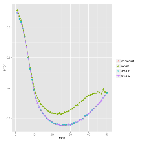
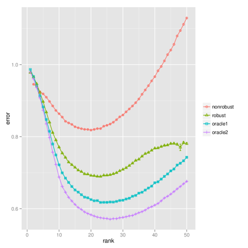
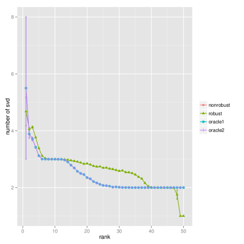
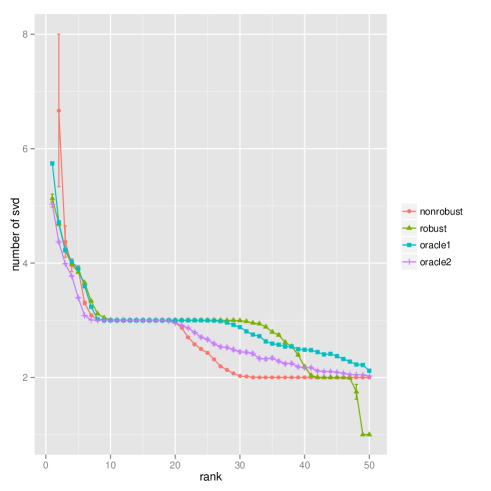
Figure 1: Top: The average test errors with their standard error bands (plus or minus one standard error). Bottom: The average number of singular value decompositions used with standard error bands (plus or minus one standard error). Left: results for the simulation setting: $r=10$, $p=0$ and $q=0.5$. Right: results for the simulation setting: $r=10$, $p=0.1$ and $q=0.5$.

5.2 Experiment 2: Image Inpainting

In this experiment the target matrix is the so-called Lena image that has been used by many authors in the image processing literature. It consists of $256\times 256$ pixels and is shown in Figure 2 (Left). The simulated data sets were generated via contaminating this Lena image by adding Gaussian noises and/or outliers in the following manner. First independent Gaussian noise was added to each pixel, where the standard deviation of the noise was set such that the SNR is 3. Next, 10% of the pixels were selected as outliers, and to them additional independent Gaussian noises with SNR 3/4 were added. In terms of selecting missing pixels, two mechanisms were considered. In the first one 40% of the pixels were randomly chosen as missing pixels, while in the second mechanism only 10% were missing but they were clustered together to form patches. Two typical simulated data sets are shown in Figure 2 (Middle). Note that Theorem 2 does not cover the second missing mechanism. For each missing mechanism, 200 data sets were generated and both Soft-Impute and Robust-Impute were applied to reconstruct Lena.

The average training and testing errors of the recovered images of matrix ranks 50, 75, 100 and 125 are reported in Table 1. For both missing mechanisms, Soft-Impute tends to have lower training errors, but larger testing errors when compared to Robust-Impute. In other words, Soft-Impute tends to over-fit the data, and Robust-Impute seems to provide better results. Lastly, for visual evaluation, the recovered image of rank 100 using Robust-Impute is displayed in Figure 1 (Right). From this one can see that the proposed Robust-Impute provided good recoveries under both missing mechanisms.

Table 1: The average training and testing errors for the Lena experiment.

		training error				testing error
	rank	50	75	100	125	50	75	100	125
independent	Soft-Impute	0.0499	0.0351	0.0221	0.0113	0.0578	0.0565	0.0581	0.0620
missing	Robust-Impute	0.0486	0.0371	0.0282	0.0252	0.0546	0.0540	0.0557	0.0571
clustered	Soft-Impute	0.0487	0.0386	0.0296	0.0214	0.0756	0.0751	0.0760	0.0781
missing	Robust-Impute	0.0468	0.0390	0.0321	0.0268	0.0716	0.0714	0.0723	0.0742

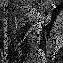
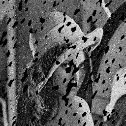
Figure 2: Left: the Lena image. Middle: degraded Lena images by the independent missing mechanism (Top) and the clustered missing mechanism (Down). Right: corresponding recovered images of rank 100 via Robust-Impute.

5.3 Real data application: Landsat Thematic Mapper

In this application the target matrix is an image from a Landsat Thematic Mapper data set publicly available at http://ternauscover.science.uq.edu.au/. This data set contains 149 multiband images of $100\times 100$ pixels, with each image consists of six bands (blue, green and red with three infrared bands). The scene is centered on the Tumbarumba flux tower on the western slopes of the Snowy Mountains in Australia. Due to wild fires or related reasons, some pixels are of value zero which can be treated as missing. Also, due to detector malfunctioning, some isolated pixels have values much higher than the remaining pixels, which can be treated as outliers. We selected an image band with a high missing rate (27.6%) to test our procedure.

To evaluate the recovered matrix, the observed pixels were split into training, validation and testing sets consisting 80%, 10% and 10% of the observed (nonzero) entries respectively. We used the validation set to tune $\gamma$. The validation errors are computed in two ways: mean squared error (MSE) $\sqrt{\sum_{(i,j)\in\mathcal{V}}(X_{ij}-\hat{X}_{ij})^{2}/|\mathcal{V}|}$ and mean absolute deviation (MAD) $\mathrm{median}\{|X_{ij}-\hat{X}_{ij}|:(i,j)\in\mathcal{V}\}$, where $\mathcal{V}$ represents the validation set. Similarly, we compute the testing errors in terms of MSE and MAD. Note that the validation and testing sets may contain outliers and therefore MAD serves as a robust and reliable performance measure. The corresponding results are shown in Table 2. From this table it can be seen that with the presence of outliers, Robust-Imputeprovided better results.

Table 2: Rank and testing errors of the real data application.

	tuning by MSE			tuning by MAD
	rank	MSE	MAD	rank	MSE	MAD
Soft-Impute	24	45.20	31.15	21	45.23	31.15
Robust-Impute	24	44.63	29.00	29	44.57	28.76

6 Concluding remarks

In this paper a classical idea from robust statistics has been brought to the matrix completion problem. The result is a new matrix completion method that can handle noisy and outlying entries. This method uses the Huber function to downweigh the effects of outliers. A new algorithm is developed to solve the corresponding optimization problem. This algorithm is relatively fast, easy to implement and monotonic convergent. It can be paired with any existing (non-robust) matrix completion methods to make such methods robust against outliers. We also developed a specialized version of this algorithm, called Robust-Impute. Its promising empirical performance has been illustrated via numerical experiments. Lastly, we have shown that the proposed method is stable; that is, with high probability, the error of recovered matrix is bounded by a constant proportional to the noise level.

Appendix A Technical Details

A.1 Proofs of Proposition 1

Proof.

By rewriting

$$\begin{split}\|\mathcal{P}_{\Omega_{{\rm obs}}}{Z}^{(k+1)}-\mathcal{P}_{\Omega_{{\rm obs}}}{Y}^{(k+1)}\|_{F}^{2}&=\|\mathcal{P}_{\Omega_{{\rm obs}}}{Z}^{(k+1)}-\mathcal{P}_{\Omega_{{\rm obs}}}{Y}^{(k)}\|_{F}^{2}+\|\mathcal{P}_{\Omega_{{\rm obs}}}{Y}^{(k)}-\mathcal{P}_{\Omega_{{\rm obs}}}{Y}^{(k+1)}\|_{F}^{2}\\ &\quad 2\times\mathrm{trace}\left[\{\mathcal{P}_{\Omega_{{\rm obs}}}{Z}^{(k+1)}-\mathcal{P}_{\Omega_{{\rm obs}}}{Y}^{(k)}\}\{\mathcal{P}_{\Omega_{{\rm obs}}}{Y}^{(k)}-\mathcal{P}_{\Omega_{{\rm obs}}}{Y}^{(k+1)}\}^{\intercal}\right],\end{split}$$

and using $f(Y^{(k+1)}|Z^{(k+1)})\leq f(Y^{(k)}|Z^{(k+1)})$, we have

$$\begin{split}&\frac{1}{2}\|\mathcal{P}_{\Omega_{{\rm obs}}}{Y}^{(k)}-\mathcal{P}_{\Omega_{{\rm obs}}}{Y}^{(k+1)}\|_{F}^{2}+\mathrm{trace}\left[\{\mathcal{P}_{\Omega_{{\rm obs}}}{Z}^{(k+1)}-\mathcal{P}_{\Omega_{{\rm obs}}}{Y}^{(k)}\}\{\mathcal{P}_{\Omega_{{\rm obs}}}{Y}^{(k)}-\mathcal{P}_{\Omega_{{\rm obs}}}{Y}^{(k+1)}\}^{\intercal}\right]\\ &\quad+\gamma\|{Y}^{(k+1)}\|_{*}\leq\gamma\|{Y}^{(k)}\|_{*}.\end{split}$$

Thus, by substituting $Z^{(k+1)}=\mathcal{P}_{\Omega_{{\rm obs}}}{Y}^{(k)}+\frac{1}{2}\rho_{c}^{\prime}(\mathcal{P}_{\Omega_{{\rm obs}}}{X}-\mathcal{P}_{\Omega_{{\rm obs}}}{Y}^{(k)})$,

$$\begin{split}&\frac{1}{2}\|\mathcal{P}_{\Omega_{{\rm obs}}}{Y}^{(k)}-\mathcal{P}_{\Omega_{{\rm obs}}}{Y}^{(k+1)}\|_{F}^{2}+\frac{1}{2}\mathrm{trace}\left[\rho^{\prime}_{c}(\mathcal{P}_{\Omega_{{\rm obs}}}{X}-\mathcal{P}_{\Omega_{{\rm obs}}}{Y}^{(k)})\{\mathcal{P}_{\Omega_{{\rm obs}}}{Y}^{(k)}-\mathcal{P}_{\Omega_{{\rm obs}}}{Y}^{(k+1)}\}^{\intercal}\right]\\ &\quad+\gamma\|{Y}^{(k+1)}\|_{*}\leq\gamma\|{Y}^{(k)}\|_{*}.\end{split}$$ (10)

Here we abuse the notation slightly so that $\rho^{\prime}_{c}$ of a matrix simply means the matrix formed by applying $\rho^{\prime}_{c}$ to its entries. Note that for each $(i,j)\in\Omega_{{\rm obs}}$, by Taylor’s expansion,

$$\rho_{c}(X_{ij}-Y_{ij}^{(k+1)}) =\rho(X_{ij}-Y_{ij}^{(k)})+(Y_{ij}^{(k)}-Y_{ij}^{(k)})\rho^{\prime}_{c}(X_{ij}-Y_{ij}^{(k)})+\int^{X_{ij}-Y_{ij}^{(k+1)}}_{X_{ij}-Y_{ij}^{(k)}}(X_{ij}-Y_{ij}^{(k+1)}-t)\rho_{c}^{\prime\prime}(t)dt,$$

and the last integral term is less than or equal to $(Y_{ij}^{(k)}-Y_{ij}^{(k+1)})^{2}$ due to $\rho_{c}^{\prime\prime}\leq 2$ almost everywhere. Thus,

$$\begin{split}\sum_{(i,j)\in\Omega_{{\rm obs}}}\rho_{c}(X_{ij}-Y_{ij}^{(k+1)})&\leq\sum_{(i,j)\in\Omega_{{\rm obs}}}\rho_{c}(X_{ij}-Y_{ij}^{(k)})\\ &\quad+\mathrm{trace}\left[\rho_{c}^{\prime}(\mathcal{P}_{\Omega_{{\rm obs}}}{X}-\mathcal{P}_{\Omega_{{\rm obs}}}{Y}^{(k)})\{\mathcal{P}_{\Omega_{{\rm obs}}}{Y}^{(k)}-\mathcal{P}_{\Omega_{{\rm obs}}}{Y}^{(k+1)}\}^{\intercal}\right]\\ &\quad+\|\mathcal{P}_{\Omega_{{\rm obs}}}{Y}^{(k)}-\mathcal{P}_{\Omega_{{\rm obs}}}{Y}^{(k+1)}\|_{F}^{2}.\end{split}$$

Now, plugging it into (10), we have $g({Y}^{(k+1)})\leq g({Y}^{(k)})$. ∎

Alternative proof of Proposition 1.

Similar to the proof of Proposition 2 in Section A.3, one can show that

$$g(Y)=\min_{S}\frac{1}{2}\|\mathcal{P}_{\Omega_{{\rm obs}}}X-\mathcal{P}_{\Omega_{{\rm obs}}}Y-\mathcal{P}_{\Omega_{{\rm obs}}}S\|_{F}^{2}+\gamma\|Y\|_{*}+c\|S\|_{1},$$ (11)

where the minimizer is $S(Y)=(1/2)\psi_{c}(\mathcal{P}_{\Omega_{{\rm obs}}}X-\mathcal{P}_{\Omega_{{\rm obs}}}Y)$. Now, one can show that

$$Z^{(k+1)} =\mathcal{P}_{\Omega_{{\rm obs}}}Y^{(k)}+(1/2)\psi_{c}(\mathcal{P}_{\Omega_{{\rm obs}}}X-\mathcal{P}_{\Omega_{{\rm obs}}}Y^{(k)})$$

$$=\mathcal{P}_{\Omega_{{\rm obs}}}X+(1/2)\psi_{c}(\mathcal{P}_{\Omega_{{\rm obs}}}Y^{(k)}-\mathcal{P}_{\Omega_{{\rm obs}}}X)$$

$$=\mathcal{P}_{\Omega_{{\rm obs}}}X-(1/2)\psi_{c}(\mathcal{P}_{\Omega_{{\rm obs}}}X-\mathcal{P}_{\Omega_{{\rm obs}}}Y^{(k)})$$

$$=\mathcal{P}_{\Omega_{{\rm obs}}}X-S(Y^{(k)}).$$

Now, due to (11),

$$g(Y^{(k+1)}) =\min_{S}\frac{1}{2}\|\mathcal{P}_{\Omega_{{\rm obs}}}X-\mathcal{P}_{\Omega_{{\rm obs}}}Y^{(k+1)}-\mathcal{P}_{\Omega_{{\rm obs}}}S\|_{F}^{2}+\gamma\|Y^{(k+1)}\|_{*}+c\|S\|_{1}$$

$$\leq\frac{1}{2}\|\mathcal{P}_{\Omega_{{\rm obs}}}X-\mathcal{P}_{\Omega_{{\rm obs}}}Y^{(k+1)}-\mathcal{P}_{\Omega_{{\rm obs}}}S(Y^{(k)})\|_{F}^{2}+\gamma\|Y^{(k+1)}\|_{*}+c\|S(Y^{(k)})\|_{1}$$

$$=f(Y^{(k+1)}|X-S(Y^{(k)}))+c\|S(Y^{(k)})\|_{1}$$

$$=f(Y^{(k+1)}|\mathcal{P}_{\Omega_{{\rm obs}}}X-S(Y^{(k)}))+c\|S(Y^{(k)})\|_{1}$$

$$=f(Y^{(k+1)}|Z^{(k+1)})+c\|S(Y^{(k)})\|_{1}$$

$$\leq f(Y^{(k)}|Z^{(k+1)})+c\|S(Y^{(k)})\|_{1}$$

$$=\frac{1}{2}\|\mathcal{P}_{\Omega_{{\rm obs}}}X-\mathcal{P}_{\Omega_{{\rm obs}}}Y^{(k)}-\mathcal{P}_{\Omega_{{\rm obs}}}S(Y^{(k)})\|_{F}^{2}+\gamma\|Y^{(k)}\|_{*}+c\|S(Y^{(k)})\|_{1}$$

$$=g(Y^{(k)}).$$

∎

A.2 Proof of Theorem 1 for Algorithm 1

Proof.

This proof closely follows the proofs of Lemma 2.3 and Theorem 3.1 in Beck and Teboulle (2009) by modifying their approximation model to

$$\zeta({Y},\tilde{{Y}}) =g_{1}(\tilde{Y})+\langle{Y}-\tilde{Y},\nabla g_{1}(\tilde{Y})\rangle+\frac{1}{2}\|\mathcal{P}_{\Omega_{{\rm obs}}}{Y}-\mathcal{P}_{\Omega_{{\rm obs}}}\tilde{Y}\|_{F}^{2}+g_{2}({Y})$$

$$=g_{1}(\tilde{Y})-\frac{1}{2}\langle{Y}-\tilde{Y},\psi_{c}(\mathcal{P}_{\Omega_{{\rm obs}}}{X}-\mathcal{P}_{\Omega_{{\rm obs}}}\tilde{Y})\rangle+\frac{1}{2}\|\mathcal{P}_{\Omega_{{\rm obs}}}{Y}-\mathcal{P}_{\Omega_{{\rm obs}}}\tilde{Y}\|_{F}^{2}+g_{2}({Y})$$

$$=g_{1}(\tilde{Y})-\frac{1}{2}\langle\mathcal{P}_{\Omega_{{\rm obs}}}{Y}-\mathcal{P}_{\Omega_{{\rm obs}}}\tilde{Y},\psi_{c}(\mathcal{P}_{\Omega_{{\rm obs}}}{X}-\mathcal{P}_{\Omega_{{\rm obs}}}\tilde{Y})\rangle+\frac{1}{2}\|\mathcal{P}_{\Omega_{{\rm obs}}}{Y}-\mathcal{P}_{\Omega_{{\rm obs}}}\tilde{Y}\|_{F}^{2}+g_{2}({Y}),$$

where $\langle{X},{Y}\rangle=\sum_{i,j}{X}_{ij}{Y}_{ij}$. It can be shown that $\arg\min_{Y}\zeta(Y,\tilde{Y})$ is the same as $\arg\min_{Y}f(Y|Z)$, where $Z=\mathcal{P}_{\Omega_{{\rm obs}}}\tilde{Y}+(1/2)\psi_{c}(\mathcal{P}_{\Omega_{{\rm obs}}}X-\mathcal{P}_{\Omega_{{\rm obs}}}\tilde{Y})$, in Steps 2(a)-(c) of Algorithm 1. Let $\Pi(\tilde{Y})=\arg\min_{Y}\zeta({Y},\tilde{Y})$. Therefore ${Y}^{(k+1)}=\Pi({Y}^{(k)})$. Moreover,

$$g_{1}({Y})\leq g_{1}(\tilde{Y})+\langle{Y}-\tilde{Y},\nabla g_{1}(\tilde{Y})\rangle+\frac{1}{2}\|\mathcal{P}_{\Omega_{{\rm obs}}}{Y}-\mathcal{P}_{\Omega_{{\rm obs}}}\tilde{Y}\|_{F}^{2},$$

for any ${Y}$ and $\tilde{Y}$. Therefore, $g(\Pi(\tilde{Y}))\leq\zeta(\Pi(\tilde{Y}),\tilde{Y})$ for any $\tilde{Y}\in\mathbb{R}^{n_{1}\times n_{2}}$.

To proceed, we need a modified version of Lemma 2.3 in Beck and Teboulle (2009).

Lemma 1.

For any $\tilde{Y},{Y}\in\mathbb{R}^{n_{1}\times n_{2}}$,

$$g({Y})-g(\Pi(\tilde{Y}))\geq\frac{1}{2}\|\mathcal{P}_{\Omega_{{\rm obs}}}\Pi(\tilde{Y})-\mathcal{P}_{\Omega_{{\rm obs}}}\tilde{Y}\|_{F}^{2}+\langle\mathcal{P}_{\Omega_{{\rm obs}}}\tilde{Y}-\mathcal{P}_{\Omega_{{\rm obs}}}{Y},\mathcal{P}_{\Omega_{{\rm obs}}}\Pi(\tilde{Y})-\mathcal{P}_{\Omega_{{\rm obs}}}{Y}\rangle.$$

This lemma is proved as follows. Since $\Pi(\tilde{Y})$ is the minimizer of the convex function $\zeta(\cdot,\tilde{Y})$, there exists a $b(\tilde{Y})\in\partial g_{2}(\Pi(\tilde{Y}))$, the subdifferential of $g_{2}$ at $\Pi(\tilde{Y})$, such that $\nabla g_{1}(\tilde{Y})+\mathcal{P}_{\Omega_{{\rm obs}}}\Pi(\tilde{Y})-\mathcal{P}_{\Omega_{{\rm obs}}}\tilde{Y}+b(\tilde{Y})=0$. By the convexity of $g_{1}$ and $g_{2}$,

$$g_{1}({Y}) \geq g_{1}(\tilde{Y})-\frac{1}{2}\langle{Y}-\tilde{Y},\psi_{c}(\mathcal{P}_{\Omega_{{\rm obs}}}X-\mathcal{P}_{\Omega_{{\rm obs}}}\tilde{Y})\rangle$$

$$g_{2}({Y}) \geq g_{2}(\Pi(\tilde{Y}))-\langle{Y}-\Pi(\tilde{Y}),b(\tilde{Y})\rangle.$$

Therefore,

$$g({Y})\geq g_{1}(\tilde{Y})-\frac{1}{2}\langle{Y}-\tilde{Y},\psi_{c}(\mathcal{P}_{\Omega_{{\rm obs}}}X-\mathcal{P}_{\Omega_{{\rm obs}}}\tilde{Y})\rangle+g_{2}(\Pi(\tilde{Y}))-\langle{Y}-\Pi(\tilde{Y}),b(\tilde{Y})\rangle.$$ (12)

Since $g(\Pi(\tilde{Y}))\leq\zeta(\Pi(\tilde{Y}),\tilde{Y})$, we have $g({Y})-g(\Pi(\tilde{Y}))\geq g(Y)-\zeta(\Pi(\tilde{Y}),\tilde{Y})$. Plugging in (12), the definition of $\zeta$ and the condition for $b$, the conclusion of the lemma follows.

Using Lemma 1 with ${Y}={Y}^{*}$ and $\tilde{Y}={Y}^{(k)}$, we have

$$2\{g({Y}^{*})-g({Y}^{(k)})\}\geq\|\mathcal{P}_{\Omega_{{\rm obs}}}{Y}^{*}-\mathcal{P}_{\Omega_{{\rm obs}}}{Y}^{(k+1)}\|_{F}^{2}-\|\mathcal{P}_{\Omega_{{\rm obs}}}{Y}^{*}-\mathcal{P}_{\Omega_{{\rm obs}}}{Y}^{(k)}\|_{F}^{2}.$$

Summing it over $k=0,\dots,m-1$,

$$2\left\{mg({Y}^{*})-\sum^{m-1}_{k=0}g({Y}^{(k)})\right\}\geq\|\mathcal{P}_{\Omega_{{\rm obs}}}{Y}^{*}-\mathcal{P}_{\Omega_{{\rm obs}}}{Y}^{(m)}\|_{F}^{2}-\|\mathcal{P}_{\Omega_{{\rm obs}}}{Y}^{*}-\mathcal{P}_{\Omega_{{\rm obs}}}{Y}^{(0)}\|_{F}^{2}.$$ (13)

Applying Lemma 1 with ${Y}=\tilde{Y}={Y}^{(k)}$,

$$2\left\{g({Y}^{(k)})-g({Y}^{(k+1)})\right\}\geq\|\mathcal{P}_{\Omega_{{\rm obs}}}{Y}^{(k+1)}-\mathcal{P}_{\Omega_{{\rm obs}}}{Y}^{(k)}\|_{F}^{2}.$$

Multiplying it by $k$ and summing over $k=0,\dots,m-1$,

$$2\left\{-mg({Y}^{(m)})+\sum^{m-1}_{k=0}g({Y}^{(k+1)})\right\}\geq\sum^{m-1}_{k=0}k\|\mathcal{P}_{\Omega_{{\rm obs}}}{Y}^{(k+1)}-\mathcal{P}_{\Omega_{{\rm obs}}}{Y}^{(k)}\|_{F}^{2}.$$ (14)

Adding (13) and (14),

$$\begin{split}2\left\{g({Y}^{*})-g({Y}^{(m)})\right\}&\geq\|\mathcal{P}_{\Omega_{{\rm obs}}}{Y}^{*}-\mathcal{P}_{\Omega_{{\rm obs}}}{Y}^{(m)}\|_{F}^{2}-\|\mathcal{P}_{\Omega_{{\rm obs}}}{Y}^{*}-\mathcal{P}_{\Omega_{{\rm obs}}}{Y}^{(0)}\|_{F}^{2}\\ &\quad+\sum^{m-1}_{k=0}k\|\mathcal{P}_{\Omega_{{\rm obs}}}{Y}^{(k+1)}-\mathcal{P}_{\Omega_{{\rm obs}}}{Y}^{(k)}\|_{F}^{2}.\end{split}$$

Therefore,

$$g({Y}^{(m)})-g({Y}^{*})\leq\frac{\|\mathcal{P}_{\Omega_{{\rm obs}}}{Y}^{*}-\mathcal{P}_{\Omega_{{\rm obs}}}Y^{(0)}\|_{F}^{2}}{2m}.$$

∎

A.3 Proof of Proposition 2

Proof.

Since both (2) and (7) are convex, we only need to consider the sub-gradients. The sub-gradient conditions for minimizier of (2) are given as follows:

$$0 \in-\frac{1}{2}\rho^{\prime}_{c}(\mathcal{P}_{\Omega_{{\rm obs}}}{X}-\mathcal{P}_{\Omega_{{\rm obs}}}{Y})+\gamma\partial\|{Y}\|_{*},$$ (15)

where $\partial\|\cdot\|_{*}$ represents the set of subgradients of the nuclear norm. The sub-gradient conditions for minimizier of (7) are given as follows:

$${0} \in-\mathcal{P}_{\Omega_{{\rm obs}}}({X}-L-S)+\gamma\partial\|L\|_{*}$$ (16)

$${0} \in-\mathcal{P}_{\Omega_{{\rm obs}}}({X}-L-S)+c\partial\|S\|_{1},$$ (17)

where $\partial\|\cdot\|_{1}$ represents the set of subgradients of $\|\cdot\|_{1}$. Here (17) implies, for $(i,j)\in\Omega_{{\rm obs}}$,

$$S_{ij}=\begin{cases}X_{ij}-L_{ij}-c,&X_{ij}-L_{ij}>c\\ 0,&|X_{ij}-L_{ij}|\leq c\\ X_{ij}-L_{ij}+c,&X_{ij}-L_{ij}<-c\end{cases}$$ (18)

and $S_{ij}=0$ for $(i,j)\in\Omega_{{\rm obs}}^{\perp}$. Note, for $(i,j)\in\Omega_{{\rm obs}}$, $X_{ij}-L_{ij}-S_{ij}=\rho_{c}^{\prime}(X_{ij}-L_{ij})/2$. Plugging it into (16), we have (15) and thus this proves the proposition. ∎

A.4 Proof of Theorem 2

To prove Theorem 2, we first show three lemmas and one proposition.

Lemma 2 (Modified Lemma A.2 in (Candès et al., 2011)).

Assume that for any matrix $Q$, $\|\mathcal{P}_{T}\mathcal{P}_{\Gamma^{\perp}}Q\|_{F}\leq n\|\mathcal{P}_{T^{\perp}}\mathcal{P}_{\Gamma^{\perp}}Q\|_{F}$. Suppose there is a pair $(W,F)$ obeying

$$\begin{cases}\mathcal{P}_{T}W=0,\quad\|W\|<1/2,\\ \mathcal{P}_{\Gamma^{\perp}}F=0,\quad\|F\|_{\infty}<1/2,\\ UV^{\intercal}+W+\mathcal{P}_{T}D=\lambda(\mathrm{sgn}(S_{0}^{\prime})+F)\quad\mathrm{with}\quad\|\mathcal{P}_{T}D\|_{F}\leq n^{-2}.\end{cases}$$ (19)

Then for any perturbation $H=(H_{L},H_{S})$ satisfying $\mathcal{P}_{\Omega_{{\rm obs}}}H_{L}+\mathcal{P}_{\Omega_{{\rm obs}}}H_{S}=0$,

$$\|M_{0}-H\|_{\Diamond}\geq\|M_{0}\|_{\Diamond}+\left(\frac{1}{2}-\frac{1}{n}\right)\|\mathcal{P}_{T^{\perp}}H_{L}\|_{*}+\left(\frac{\lambda}{2}-\frac{n+1}{n^{2}}\right)\|\mathcal{P}_{\Gamma}H_{L}\|_{1}.$$

The proof of this lemma can be found in Candès et al. (2011). To procced, we write $\|M\|_{F,\lambda}^{2}=\|L\|_{F}^{2}+\lambda^{2}\|S\|_{F}^{2}$ for any pair of matrices $M=(L,S)$.

Lemma 3.

Let $M=(M_{L},M_{S})$ be any pair of matrices. Suppose $\|\mathcal{P}_{\Omega_{{\rm obs}}}\mathcal{P}_{T}M_{L}\|_{F}^{2}\geq p_{0}\|\mathcal{P}_{T}M_{L}\|_{F}^{2}/2$ and $\|\mathcal{P}_{T}\mathcal{P}_{\Omega}\|^{2}\leq p_{0}/8$. Then

$$\|\mathcal{P}_{\Psi}(\mathcal{P}_{T}\times\mathcal{P}_{\Omega})M\|_{F,\lambda}^{2}\geq\frac{(1+\lambda^{2})p_{0}}{16}\|(\mathcal{P}_{T}\times\mathcal{P}_{\Omega})M\|_{F}^{2}.$$

Proof of Lemma 3.

Note that for any $M^{\prime}=(M^{\prime}_{L},M_{S}^{\prime})$,

$$\mathcal{P}_{\Psi}M^{\prime}=\left(\frac{\mathcal{P}_{\Omega_{{\rm obs}}}(M_{L}^{\prime}+M_{S}^{\prime})}{2},\frac{\mathcal{P}_{\Omega_{{\rm obs}}}(M_{L}^{\prime}+M_{S}^{\prime})}{2}\right).$$

Thus

$$\|\mathcal{P}_{\Psi}(\mathcal{P}_{T}\times\mathcal{P}_{\Omega})M\|_{F,\lambda}^{2} =\frac{1+\lambda^{2}}{4}\|\mathcal{P}_{\Omega_{{\rm obs}}}(\mathcal{P}_{T}M_{L}+\mathcal{P}_{\Omega}M_{S})\|_{F}^{2}$$

$$=\frac{1+\lambda^{2}}{4}\left(\|\mathcal{P}_{\Omega_{{\rm obs}}}\mathcal{P}_{T}M_{L}\|_{F}^{2}+\|\mathcal{P}_{\Omega}M_{S}\|_{F}^{2}+2\langle\mathcal{P}_{\Omega_{{\rm obs}}}\mathcal{P}_{T}M_{L},\mathcal{P}_{\Omega}M_{S}\rangle\right),$$

where the last equality is due to $\Omega\subset\Omega_{{\rm obs}}$. By $\|\mathcal{P}_{T}\mathcal{P}_{\Omega}\|^{2}\leq p_{0}/8$,

$$\langle\mathcal{P}_{\Omega_{{\rm obs}}}\mathcal{P}_{T}M_{L},\mathcal{P}_{\Omega}M_{S}\rangle =\langle\mathcal{P}_{T}M_{L},\mathcal{P}_{\Omega}M_{S}\rangle$$

$$=\langle\mathcal{P}_{T}M_{L},(\mathcal{P}_{T}\mathcal{P}_{\Omega})\mathcal{P}_{\Omega}M_{S}\rangle$$

$$\geq-\|\mathcal{P}_{T}\mathcal{P}_{\Omega}\|\|\mathcal{P}_{T}M_{L}\|_{F}\|\mathcal{P}_{\Omega}M_{S}\|_{F}$$

$$\geq-\frac{\sqrt{p_{0}}}{2\sqrt{2}}\|\mathcal{P}_{T}M_{L}\|_{F}\|\mathcal{P}_{\Omega}M_{S}\|_{F}.$$

Combining with $\|\mathcal{P}_{\Omega_{{\rm obs}}}\mathcal{P}_{T}M_{L}\|_{F}^{2}\geq p_{0}\|\mathcal{P}_{T}M_{L}\|_{F}^{2}/2$, we have

$$\|\mathcal{P}_{\Psi}(\mathcal{P}_{T}\times\mathcal{P}_{\Omega})M\|_{F,\lambda}^{2}\geq\frac{1+\lambda^{2}}{4}\left(\frac{p_{0}}{2}\|\mathcal{P}_{T}M_{L}\|_{F}^{2}+\|\mathcal{P}_{\Omega}M_{S}\|_{F}^{2}-\sqrt{\frac{{p_{0}}}{{2}}}\|\mathcal{P}_{T}M_{L}\|_{F}\|\mathcal{P}_{\Omega}M_{S}\|_{F}\right).$$

As $2(x^{2}+y^{2}-xy)\geq x^{2}+y^{2}$ for $x,y\geq 0$,

$$\|\mathcal{P}_{\Psi}(\mathcal{P}_{T}\times\mathcal{P}_{\Omega})M\|_{F,\lambda}^{2}\geq\frac{1+\lambda^{2}}{8}\left(\frac{p_{0}}{2}\|\mathcal{P}_{T}M_{L}\|_{F}^{2}+\|\mathcal{P}_{\Omega}M_{S}\|_{F}^{2}\right)\geq\frac{(1+\lambda^{2})p_{0}}{16}\|(\mathcal{P}_{T}\times\mathcal{P}_{\Omega})M\|_{F}^{2}.$$

∎

Lemma 4.

Let $M=(M_{L},M_{S})$ be any pair of matrices. Then $\|\mathcal{P}_{\Psi}M\|_{F,\lambda}^{2}\leq\|M\|_{F,\lambda}^{2}/2$.

Proof of Lemma 4.

Write $M^{\Psi}=(M^{\Psi}_{L},M^{\Psi}_{S})=\mathcal{P}_{\Psi}M$. Since $\|M^{\Psi}_{L}\|_{F}^{2}=\|M^{\Psi}_{S}\|_{F}^{2}$,

$$\|\mathcal{P}_{\Psi}M\|_{F,\lambda}^{2} =\|M^{\Psi}_{L}\|_{F}^{2}+\lambda^{2}\|M^{\Psi}_{S}\|_{F}^{2}$$

$$=\frac{1}{2}(\|M^{\Psi}_{L}\|_{F}^{2}+\|M^{\Psi}_{S}\|_{F}^{2})+\frac{\lambda^{2}}{2}(\|M^{\Psi}_{L}\|_{F}^{2}+\|M^{\Psi}_{S}\|_{F}^{2})$$

$$=\frac{1}{2}\|M^{\Psi}\|_{F}^{2}+\frac{\lambda^{2}}{2}\|M^{\Psi}\|_{F}^{2}$$

$$\leq\frac{1}{2}\|M\|_{F}^{2}+\frac{\lambda^{2}}{2}\|M\|_{F}^{2}=\frac{1}{2}\|M\|_{F,\lambda}^{2}.$$

∎

Proposition 3.

Assume that for any matrix $Q$, $\|\mathcal{P}_{T}\mathcal{P}_{\Gamma^{\perp}}Q\|_{F}\leq n\|\mathcal{P}_{T^{\perp}}\mathcal{P}_{\Gamma^{\perp}}Q\|_{F}$ and $\|\mathcal{P}_{\Omega_{{\rm obs}}}\mathcal{P}_{T}Q\|_{F}\geq p_{0}\|\mathcal{P}_{T}Q\|_{F}/2$. Further suppose $4/n<\lambda\leq 1$, $n\geq 3$, $p_{0}>0$, $\|\mathcal{P}_{T}\mathcal{P}_{\Omega}\|^{2}\leq p_{0}/8$ and that there exists a pair $(W,F)$ obeying (19). Then the solution $\hat{M}=(\hat{L},\hat{S})$ to (7) satisfies

$$\|\hat{M}-M_{0}\|_{F,\lambda}\leq\left[\sqrt{1+\lambda^{2}}+4\left(1+\sqrt{\frac{8}{{p_{0}}}}\right)(\sqrt{n}+n\lambda\sqrt{p_{0}})\right]\delta.$$

where $M_{0}=(L_{0},S_{0}^{\prime})$ such that $\|\mathcal{P}_{\Omega_{{\rm obs}}}X-\mathcal{P}_{\Omega_{{\rm obs}}}(L_{0}+S_{0}))\|_{F}^{2}\leq\delta$ and $S_{0}^{\prime}=\mathcal{P}_{\Omega_{{\rm obs}}}S_{0}$. Further, if $\lambda=1/\sqrt{np_{0}}$ (which implies $1/n<p_{0}<n/16$), we obtain

$$\|\hat{L}-L\|_{F}\leq\left\{2+8\sqrt{n}\left(1+\sqrt{\frac{8}{{p_{0}}}}\right)\right\}\delta\qquad\mbox{and}\qquad\|\hat{S}-S_{0}^{\prime}\|_{F}\leq\left\{2+8\sqrt{n}\left(1+\sqrt{\frac{8}{{p_{0}}}}\right)\right\}\sqrt{np_{0}}\delta.$$

Proof of Proposition 3.

Write $\hat{M}=M_{0}+H$, where $H=(H_{L},H_{S})$, and $H^{\Psi}=(H^{\Psi}_{L},H^{\Psi}_{S})=\mathcal{P}_{\Psi}H$ and $H^{\Psi^{\perp}}=(H^{\Psi^{\perp}}_{L},H^{\Psi^{\perp}}_{S})=\mathcal{P}_{\Psi^{\perp}}H$. We want to bound

$$\|H\|_{F,\lambda} =\|H^{\Psi}+H^{\Psi^{\perp}}\|_{F,\lambda}$$

$$\leq\|H^{\Psi}\|_{F,\lambda}+\|H^{\Psi^{\perp}}\|_{F,\lambda}$$

$$\leq\|H^{\Psi}\|_{F,\lambda}+\|(\mathcal{P}_{T^{\perp}}\times\mathcal{P}_{\Gamma})H^{\Psi^{\perp}}\|_{F,\lambda}+\|(\mathcal{P}_{T}\times\mathcal{P}_{\Gamma^{\perp}})H^{\Psi^{\perp}}\|_{F,\lambda}.$$ (20)

We start with the first term of (20). Since $H^{\Psi}_{L}=H^{\Psi}_{S}=(1/2)\mathcal{P}_{\Omega_{{\rm obs}}}(H_{L}+H_{S})$,

$$\|H^{\Psi}\|_{F,\lambda} =\frac{\sqrt{1+\lambda^{2}}}{2}\|\mathcal{P}_{\Omega_{{\rm obs}}}(H_{L}+H_{S})\|_{F}$$

$$=\frac{\sqrt{1+\lambda^{2}}}{2}\|\mathcal{P}_{\Omega_{{\rm obs}}}(\hat{L}+\hat{S}-L_{0}-S_{0}^{\prime})\|_{F}$$

$$\leq\frac{\sqrt{1+\lambda^{2}}}{2}\left(\|\mathcal{P}_{\Omega_{{\rm obs}}}(\hat{L}+\hat{S}-X)\|_{F}+\|\mathcal{P}_{\Omega_{{\rm obs}}}(L_{0}+S_{0}^{\prime}-X)\|_{F}\right)$$

$$\leq\delta\sqrt{1+\lambda^{2}},$$

where the last inequality is due to the fact that both $M_{0}$ and $\hat{M}$ are feasible.

Then we focus on the second term of (20). First, we have

$$\|M_{0}\|_{\Diamond}\geq\|\hat{M}\|_{\Diamond}=\|M_{0}+H\|_{\Diamond}\geq\|M_{0}+H^{\Psi^{\perp}}\|_{\Diamond}-\|H^{\Psi}\|_{\Diamond}.$$

By Lemma 2,

$$\|M_{0}+H^{\Psi^{\perp}}\|_{\Diamond}\geq\|M_{0}\|_{\Diamond}+a(n)\|\mathcal{P}_{T^{\perp}}H^{\Psi^{\perp}}_{L}\|_{*}+b(n,\lambda)\|\mathcal{P}_{\Gamma}H^{\Psi^{\perp}}_{L}\|_{1},$$

where

$$a(n)=\frac{1}{2}-\frac{1}{n}\quad\mbox{and}\quad b(n,\lambda)=\frac{\lambda}{2}-\frac{n+1}{n^{2}}.$$

Now, combining the above inequalities,

$$\|H^{\Psi}\|_{\Diamond}\geq a(n)\|\mathcal{P}_{T^{\perp}}H^{\Psi^{\perp}}_{L}\|_{*}+b(n,\lambda)\|\mathcal{P}_{\Gamma}H^{\Psi^{\perp}}_{L}\|_{1}.$$ (21)

By the assumption that $\lambda>4/n$ and $n\geq 3$,

$$a(n)=\frac{1}{2}-\frac{1}{n}>0\quad\mbox{and}\quad b(n,\lambda)=\frac{\lambda}{2}-\frac{n+1}{n^{2}}>\frac{2}{n}-\frac{1}{n}-\frac{1}{n^{2}}=\frac{1}{n}-\frac{1}{n^{2}}>0.$$

Therefore (21) implies $\|H^{\Psi}\|_{\Diamond}\geq a(n)\|\mathcal{P}_{T^{\perp}}H^{\Psi^{\perp}}_{L}\|_{*}$ and $\|H^{\Psi}\|_{\Diamond}\geq b(n,\lambda)\|\mathcal{P}_{\Gamma}H^{\Psi^{\perp}}_{L}\|_{1}$.

Now, we are ready to establish a bound for the second term of (20).

$$\|(\mathcal{P}_{T^{\perp}}\times\mathcal{P}_{\Gamma})H^{\Psi^{\perp}}\|_{F,\lambda} \leq\|\mathcal{P}_{T^{\perp}}H^{\Psi^{\perp}}_{L}\|_{F}+\lambda\|\mathcal{P}_{\Gamma}H^{\Psi^{\perp}}_{S}\|_{F}$$

$$\leq\|\mathcal{P}_{T^{\perp}}H^{\Psi^{\perp}}_{L}\|_{*}+\lambda\|\mathcal{P}_{\Gamma}H^{\Psi^{\perp}}_{S}\|_{1}$$

$$\leq\left\{\frac{1}{a(n)}+\frac{\lambda}{b(n,\lambda)}\right\}\|H^{\Psi}\|_{\Diamond}$$

$$\leq 4(\|H^{\Psi}_{L}\|_{*}+\lambda\|H^{\Psi}_{S}\|_{1}).$$

As for the third term of (20), we apply Lemma 3 and the bound of the second term in (20). As $\mathcal{P}_{\Psi}H^{\Psi^{\perp}}=0$, $\mathcal{P}_{\Psi}(\mathcal{P}_{T}\times\mathcal{P}_{\Gamma^{\perp}})H^{\Psi^{\perp}}+\mathcal{P}_{\Psi}(\mathcal{P}_{T^{\perp}}\times\mathcal{P}_{\Gamma})H^{\Psi^{\perp}}=0$. Therefore, due to Lemma 4,

$$\|\mathcal{P}_{\Psi}(\mathcal{P}_{T}\times\mathcal{P}_{\Gamma^{\perp}})H^{\Psi^{\perp}}\|_{F,\lambda}=\|\mathcal{P}_{\Psi}(\mathcal{P}_{T^{\perp}}\times\mathcal{P}_{\Gamma})H^{\Psi^{\perp}}\|_{F,\lambda}\leq\frac{1}{\sqrt{2}}\|(\mathcal{P}_{T^{\perp}}\times\mathcal{P}_{\Gamma})H^{\Psi^{\perp}}\|_{F,\lambda}.$$

As $\mathcal{P}_{\Omega_{{\rm obs}}^{\perp}}H_{S}$ does not affect the feasibility of $M+H$ and $H$ is chosen such that $\|M+H\|_{\Diamond}$ is minimized, thus $\mathcal{P}_{\Omega_{{\rm obs}}^{\perp}}H^{\Psi^{\perp}}_{S}=\mathcal{P}_{\Omega_{{\rm obs}}^{\perp}}H_{S}=0$ which implies $(\mathcal{P}_{T}\times\mathcal{P}_{\Gamma^{\perp}})H^{\Psi^{\perp}}=(\mathcal{P}_{T}\times\mathcal{P}_{\Omega})H^{\Psi^{\perp}}$. Thus, by Lemma 3,

$$\|(\mathcal{P}_{T}\times\mathcal{P}_{\Gamma^{\perp}})H^{\Psi^{\perp}}\|_{F} \leq\sqrt{\frac{8}{{(1+\lambda^{2})p_{0}}}}\|(\mathcal{P}_{T^{\perp}}\times\mathcal{P}_{\Gamma})H^{\Psi^{\perp}}\|_{F,\lambda}\leq\sqrt{\frac{8}{{p_{0}}}}\|(\mathcal{P}_{T^{\perp}}\times\mathcal{P}_{\Gamma})H^{\Psi^{\perp}}\|_{F,\lambda}.$$

And $\|(\mathcal{P}_{T}\times\mathcal{P}_{\Gamma^{\perp}})H^{\Psi^{\perp}}\|_{F,\lambda}\leq\|(\mathcal{P}_{T}\times\mathcal{P}_{\Gamma^{\perp}})H^{\Psi^{\perp}}\|_{F}$ as $\lambda\leq 1$.

Collecting all the above bounds for the three terms, we derive the bound for $\|H\|_{F,\lambda}$:

$$\|H\|_{F,\lambda}\leq\delta\sqrt{1+\lambda^{2}}+4\left(1+\sqrt{\frac{8}{{p_{0}}}}\right)(\|H^{\Psi}_{L}\|_{*}+\lambda\|H^{\Psi}_{S}\|_{1}).$$

Finally, $\|H^{\Psi}_{L}\|_{*}\leq\sqrt{n}\|H^{\Psi}_{L}\|_{F}$, $\|H^{\Psi}_{S}\|_{1}=\sqrt{p_{0}n^{2}}\|H^{\Psi}_{S}\|_{F}$ (since $H^{\Psi}_{S}$ is supported on $\Omega_{{\rm obs}}$) and $\|H^{\Psi}_{L}\|_{F}=\|H^{\Psi}_{S}\|=\|\mathcal{P}_{\Omega_{{\rm obs}}}(H_{L}+H_{S})\|_{F}/2\leq\delta$. Therefore,

$$\|H\|_{F,\lambda}\leq\delta\left[\sqrt{1+\lambda^{2}}+4\left(1+\sqrt{\frac{8}{{p_{0}}}}\right)(\sqrt{n}+n\lambda\sqrt{p_{0}})\right].$$

Assume that $\lambda=1/\sqrt{np_{0}}$. First we note that, due to $\lambda>4/n$, this condition imposes a reasonable coverage of $p_{0}$: $1/n<p_{0}<n/16$. Now we focus on simplifying the bound for $\|H\|_{F,\lambda}$.

$$\sqrt{1+\lambda^{2}}+4\left(1+\sqrt{\frac{8}{{p_{0}}}}\right)(\sqrt{n}+n\lambda\sqrt{p_{0}})\leq 2+8\sqrt{n}\left(1+\sqrt{\frac{8}{{p_{0}}}}\right).$$

This implies

$$\|H_{L}\|_{F}\leq\left\{2+8\sqrt{n}\left(1+\sqrt{\frac{8}{{p_{0}}}}\right)\right\}\delta\qquad\mbox{and}\qquad\|H_{S}\|_{F}\leq\left\{2+8\sqrt{n}\left(1+\sqrt{\frac{8}{{p_{0}}}}\right)\right\}\sqrt{np_{0}}\delta.$$

∎

To prove Theorem 2, we establish one additional lemma.

Lemma 5.

Suppose $\|\mathcal{P}_{T}-p_{0}^{-1}\mathcal{P}_{T}\mathcal{P}_{\Omega_{{\rm obs}}}\mathcal{P}_{T}\|\leq 1/2$. Then for any matrix $Q$,

$$\|\mathcal{P}_{\Omega_{{\rm obs}}}\mathcal{P}_{T}Q\|_{F}^{2}\geq\frac{p_{0}}{2}\|\mathcal{P}_{T}Q\|_{F}^{2}.$$

Proof of Lemma 5.

By the assumptions, for any matrix $Q$,

$$\|\mathcal{P}_{\Omega_{{\rm obs}}}\mathcal{P}_{T}Q\|_{F}^{2} =\langle\mathcal{P}_{\Omega_{{\rm obs}}}\mathcal{P}_{T}Q,\mathcal{P}_{\Omega_{{\rm obs}}}\mathcal{P}_{T}Q\rangle$$

$$=\langle\mathcal{P}_{T}Q,\mathcal{P}_{T}\mathcal{P}_{\Omega_{{\rm obs}}}\mathcal{P}_{T}Q\rangle$$

$$=p_{0}\langle\mathcal{P}_{T}Q,p_{0}^{-1}\mathcal{P}_{T}\mathcal{P}_{\Omega_{{\rm obs}}}\mathcal{P}_{T}Q\rangle$$

$$=p_{0}\left[\|\mathcal{P}_{T}{Q}\|_{F}^{2}+\langle\mathcal{P}_{T}Q,(p_{0}^{-1}\mathcal{P}_{T}\mathcal{P}_{\Omega_{{\rm obs}}}\mathcal{P}_{T}-\mathcal{P}_{T})Q\right]$$

$$\leq p_{0}\left(\|\mathcal{P}_{T}Q\|_{F}^{2}-\frac{1}{2}\|\mathcal{P}_{T}Q\|_{F}^{2}\right)$$

$$=\frac{p_{0}}{2}\|\mathcal{P}_{T}Q\|_{F}^{2}.$$

∎

Proof of Theorem 2.

Recall that we write that an event occurs with high probability if it holds with probability at least $1-\mathop{}\mathopen{}\mathcal{O}\mathopen{}(n^{-10})$. Due to the asymptotic nature of Theorem 2, we only require the conditions of Proposition 3 to hold asymptotically with large probability. By Lemma A.3 of Candès et al. (2011), $\|\mathcal{P}_{T}\mathcal{P}_{\Gamma^{\perp}}Q\|_{F}\leq n\|\mathcal{P}_{T^{\perp}}\mathcal{P}_{\Gamma^{\perp}}Q\|_{F}$ for all $Q$, with high probability. By Lemma 5 and Theorem 2.6 of Candès et al. (2011) (see also Candès and Recht, 2009, Theorem 4.1), $\|\mathcal{P}_{\Omega_{{\rm obs}}}\mathcal{P}_{T}Q\|_{F}^{2}\geq\frac{p_{0}}{2}\|\mathcal{P}_{T}Q\|_{F}^{2}$ for all $Q$, with high probability. Further, by Candès and Recht (2009), $\|\mathcal{P}_{T}\mathcal{P}_{\Omega}\|^{2}\leq p_{0}/8$ occurs with high probability. Candès et al. (2011, pp. 33-35) show that there exist dual certificates $(W,F)$ obeying (19) with high probability. For sufficiently large $n$, the conditions of $\lambda$ and $p_{0}$ in Proposition 3 are fulfilled. Therefore, Theorem 2 follows from Proposition 3. ∎

References

• Beck and Teboulle (2009) Beck, A. and M. Teboulle (2009). A fast iterative shrinkage-thresholding algorithm for linear inverse problems. SIAM Journal on Imaging Sciences 2(1), 183–202.
• Bennett and Lanning (2007) Bennett, J. and S. Lanning (2007). The netflix prize. In Proceedings of KDD cup and workshop, Volume 2007, pp.  35.
• Cai et al. (2010) Cai, J.-F., E. J. Candés, and Z. Shen (2010). A singular value thresholding algorithm for matrix completion. SIAM Journal on Optimization 20(4), 1956–1982.
• Candès et al. (2011) Candès, E. J., X. Li, Y. Ma, and J. Wright (2011). Robust principal component analysis? Journal of the ACM (JACM) 58(3), Article 11.
• Candès and Plan (2010) Candès, E. J. and Y. Plan (2010). Matrix completion with noise. Proceedings of the IEEE 98(6), 925–936.
• Candès and Recht (2009) Candès, E. J. and B. Recht (2009). Exact matrix completion via convex optimization. Foundations of Computational mathematics 9(6), 717–772.
• Chandrasekaran et al. (2011) Chandrasekaran, V., S. Sanghavi, P. A. Parrilo, and A. S. Willsky (2011). Rank-sparsity incoherence for matrix decomposition. SIAM Journal on Optimization 21(2), 572–596.
• Chen et al. (2011) Chen, Y., H. Xu, C. Caramanis, and S. Sanghavi (2011). Robust matrix completion and corrupted columns. In Proceedings of the 28th International Conference on Machine Learning (ICML-11), pp.  873–880.
• Gross (2011) Gross, D. (2011). Recovering low-rank matrices from few coefficients in any basis. IEEE Transactions on Information Theory 57(3), 1548–1566.
• Hastie et al. (2014) Hastie, T., R. Mazumder, J. Lee, and R. Zadeh (2014). Matrix completion and low-rank SVD via fast alternating least squares. Unpublished manuscript.
• Huber and Ronchetti (2011) Huber, P. J. and E. M. Ronchetti (2011). Robust Statistics (Second ed.), Volume 693. New Jersey: John Wiley & Sons.
• Hunter and Lange (2004) Hunter, D. R. and K. Lange (2004). A tutorial on mm algorithms. The American Statistician 58(1), 30–37.
• Karhunen (2011) Karhunen, J. (2011). Robust pca methods for complete and missing data. Neural Network World 21(5), 357.
• Keshavan et al. (2010a) Keshavan, R. H., A. Montanari, and S. Oh (2010a). Matrix completion from a few entries. IEEE Transactions on Information Theory 56(6), 2980–2998.
• Keshavan et al. (2010b) Keshavan, R. H., A. Montanari, and S. Oh (2010b). Matrix completion from noisy entries. Journal of Machine Learning Research 11(1), 2057–2078.
• Koltchinskii et al. (2011) Koltchinskii, V., K. Lounici, A. B. Tsybakov, et al. (2011). Nuclear-norm penalization and optimal rates for noisy low-rank matrix completion. The Annals of Statistics 39(5), 2302–2329.
• Lange (2010) Lange, K. (2010). Numerical Analysis for Statisticians. New York: Springer.
• Lange et al. (2000) Lange, K., D. R. Hunter, and I. Yang (2000). Optimization transfer using surrogate objective functions. Journal of Computational and Graphical Statistics 9(1), 1–20.
• Luttinen et al. (2012) Luttinen, J., A. Ilin, and J. Karhunen (2012). Bayesian robust pca of incomplete data. Neural processing letters 36(2), 189–202.
• Ma et al. (2011) Ma, S., D. Goldfarb, and L. Chen (2011). Fixed point and bregman iterative methods for matrix rank minimization. Mathematical Programming 128(1-2), 321–353.
• Marjanovic and Solo (2012) Marjanovic, G. and V. Solo (2012). On $l_{q}$ optimization and matrix completion. IEEE Transactions on Signal Processing 60(11), 5714–5724.
• Mazumder et al. (2010) Mazumder, R., T. Hastie, and R. Tibshirani (2010). Spectral regularization algorithms for learning large incomplete matrices. The Journal of Machine Learning Research 11, 2287–2322.
• Montanari and Oh (2010) Montanari, A. and S. Oh (2010). On positioning via distributed matrix completion. In Sensor Array and Multichannel Signal Processing Workshop (SAM), 2010 IEEE, pp.  197–200.
• Nesterov (2007) Nesterov, Y. (2007). Gradient methods for minimizing composite objective function. Technical report, CORE.
• Oh et al. (2007) Oh, H.-S., D. W. Nychka, and T. C. M. Lee (2007). The role of pseudo data for robust smoothing with application to wavelet regression. Biometrika 94(4), 893–904.
• Recht (2011) Recht, B. (2011). A simpler approach to matrix completion. The Journal of Machine Learning Research 12, 3413–3430.
• Rennie and Srebro (2005) Rennie, J. D. and N. Srebro (2005). Fast maximum margin matrix factorization for collaborative prediction. In Proceedings of the 22nd international conference on Machine learning, pp.  713–719.
• She and Owen (2011) She, Y. and A. B. Owen (2011). Outlier detection using nonconvex penalized regression. Journal of the American Statistical Association 106(494), 626–639.
• Srebro and Jaakkola (2003) Srebro, N. and T. Jaakkola (2003). Weighted low-rank approximations. In ICML, Volume 3, pp.  720–727.
• Weinberger and Saul (2006) Weinberger, K. Q. and L. K. Saul (2006). Unsupervised learning of image manifolds by semidefinite programming. International Journal of Computer Vision 70(1), 77–90.
• Zhou et al. (2010) Zhou, Z., X. Li, J. Wright, E. Candes, and Y. Ma (2010). Stable principal component pursuit. In 2010 IEEE International Symposium on Information Theory Proceedings (ISIT), pp.  1518–1522.