The International Mass Loading Service

Abstract

The International Mass Loading Service computes four loadings: a) atmospheric pressure loading; b) land water storage loading; c) oceanic tidal loading; and d) non-tidal oceanic loading. The service provides to users the mass loading time series in three forms: 1) pre-computed time series for a list of 849 space geodesy stations; 2) pre-computed time series on the global $1^{\circ}\times 1^{\circ}$ grid; and 3) on-demand Internet service for a list of stations and a time range specified by the user. The loading displacements are provided for the time period from 1979.01.01 through present, updated on an hourly basis, and have latencies 8–20 hours.

1 Introduction

Loading is a crustal deformation caused by a redistribution of air or water mass. In particular, loading caused by the redistribution of air mass is called atmospheric pressure loading, redistribution of continental water mass in a form of snow cover, soil moisture, and ground water causes continental water storage loading (sometimes also referred to as “hydrological loading”), redistribution of oceanic water mass causes ocean loading, which in turn is sub-divided into the ocean tidal and ocean non-tidal loadings. The loading deformation on average has the rms of 3 mm but may reach 60 mm ($M_{2}$ tidal ocean loading near British island). Calculation of mass loading is a computationally intensive procedure. For a case of ocean loading, the coefficients of displacement expansion can be computed once and forever. Computation of other loadings requires knowledge of surface pressure changes caused by a redistribution of air and water masses that is highly volatile and cannot be computed beforehand. Acquiring information about time series of global mass redistribution poses a serious logistical problem that impeded implementation of data reduction for mass loading.

Realizing the magnitude of logistical problem, the mass loading service at NASA Goddard Space Flight Center was established in December 2002 (Petrov and Boy 2004). The service was limited to the atmospheric pressure loading. It provided for the geodetic community the time series of 3D displacements of several hundred space geodesy stations, as well as the global displacement field at the $1^{\circ}\times 1^{\circ}$ grid. The time series were updated daily and had latency around 3 days. The service quickly became very popular and became the main source of information about atmospheric pressure loading.

Recently, a decision was made to make a deep upgrade of the service. The upgrade targeted the following areas: a) to extend the service to loading caused by land water storage and non-tidal ocean loading; b) to support high resolution models of the atmosphere and land water storage; c) to take into account effects of local topography on surface pressure in mountain regions; d) to improve latency; e) to provide a user an ability to compute loading for user-selected stations on-demand. In the rest of the paper I will describe the approaches used for this upgrade.

2 The use of high resolution models for loading computation

The original atmospheric pressure loading service used the 2D NCEP Reanalysis surface pressure field (Kalnay et al. 1996) at a regular grid with a spatial resolution $2.5^{\circ}\times 2.5^{\circ}$. Modern models have much higher resolutions: for instance, the GEOS-FP model has resolution $0.3125^{\circ}\times 0.25^{\circ}$. The traditional approach for loading computation at a point with coordinate $\vec{r}$ involved a numerical evaluation of the integral of a convolution type (Farrell 1972):

$$\begin{array}[]{lcl}\vec{u}_{r}(\vec{r},t)&=&\displaystyle\int\int\limits_{\!\!\!\!\!\!\Omega}L(\phi^{\prime},\lambda^{\prime})\,\Delta P(\vec{r}\,^{\prime},t)\,G_{\mbox{\sc r}}(\psi)\cos\phi^{\prime}d\lambda^{\prime}d\phi^{\prime}\vspace{1ex}\\ \vec{u}_{h}(\vec{r},t)&=&\displaystyle\int\int\limits_{\!\!\!\!\!\!\Omega}\vec{q}(\vec{r},\vec{r}\,^{\prime})\,L(\phi,\lambda)\,\Delta P(\vec{r}\,^{\prime},t)\,G_{\mbox{\sc h}}(\psi)\cos\phi^{\prime}d\lambda^{\prime}d\phi^{\prime},\end{array}$$ (3)

where $\Delta P(\vec{r}\,^{\prime},t)$ is the pressure caused by mass redistribution, $L(\phi,\lambda)$ — is the land-sea mask, the share of land in an elementary cell, and $G(\psi)$ are the Green’s functions defined as

$$\begin{array}[]{lcl @{\qquad\quad} lcl }\displaystyle G_{\mbox{\sc r}}(\psi)&=&\frac{\displaystyle fa}{\displaystyle g_{0}^{2}}\displaystyle\sum_{n=0}^{+\infty}h^{{}^{\prime}}_{n}P_{n}(\cos\psi)&G_{\mbox{\sc h}}(\psi)&=&-\frac{\displaystyle fa}{\displaystyle g_{0}^{2}}\displaystyle\sum_{n=1}^{+\infty}l^{{}^{\prime}}_{n}\frac{\partial P_{n}(\cos\psi)}{\partial\psi}\end{array}.$$ (5)

The problem is that this algorithm has complexity $O(d^{4})$, where $d$ is the spatial grid size, i.e. it grows very rapidly with an increase of spatial resolution. It becomes impractical to use convolution for loading computation using models with a high spatial resolution. The alternative is to use the spherical harmonic transform approach. The algorithm involves the following steps:

1. forming the pressure difference with respect to the average;

2. transforming the surface pressure field to the regular grid with a higher resolution (upgridding): $2(D+1)+1\;\times\;4(D+1)$ over latitude and longitude, where $D$ is degree of the expansion;

3. multiplying the surface pressure field with the land-sea mask defined as a share of land in a cell;

4. spherical harmonic transform of degree/order D;

5. scaling the output of the spherical harmonic transform with Love numbers $h^{\prime}_{n}$ and $l^{\prime}_{n}$ of the corresponding degree $n$:

   $$\begin{array}[]{lcl}V^{m}_{n}(t)&=&\frac{\displaystyle 1}{\displaystyle\bar{\rho}_{\oplus}\,g_{0}}\frac{\displaystyle 3h^{\prime}_{n}}{\displaystyle 2n+1}\displaystyle\int\int\limits_{\!\!\!\!\!\!\Omega}L(\phi,\lambda)\,\Delta P(t,\phi,\lambda)\,Y^{m}_{n}(\phi,\lambda)\cos\phi\,d\phi\,d\lambda\vspace{1ex}\\ H^{m}_{n}(t)&=&\frac{\displaystyle 1}{\displaystyle\bar{\rho}_{\oplus}\,g_{0}}\frac{\displaystyle 3l^{\prime}_{n}}{\displaystyle 2n+1}\displaystyle\int\int\limits_{\!\!\!\!\!\!\Omega}L(\phi,\lambda)\,\Delta P(t,\phi,\lambda)\,Y^{m}_{n}(\phi,\lambda)\cos\phi\,d\phi\,d\lambda\\ \end{array},$$ (8)

   where $\bar{\rho}_{\oplus}$ is the mean Earth’s density and $g_{0}$ is the equatorial gravity acceleration. The expression under the integral is the spherical harmonics $\left(\right){}^{m}_{n}$ of the the pressure field with the land-sea mask applied.

6. inverse spherical harmonic transform:

   $$\begin{array}[]{lcl}D_{U}(\phi,\lambda)&=&\displaystyle\sum\limits_{i=0}^{i=m}\sum\limits_{j=-n}^{j=n}V^{i}_{j}\,{Y^{i}_{j}}^{*}(\phi,\lambda)\vspace{1ex}\\ D_{E}(\phi,\lambda)&=&\displaystyle\sum\limits_{i=0}^{i=m}\sum\limits_{j=-n}^{j=n}H^{i}_{j}\,\makebox{}\frac{\partial{Y^{i}_{j}}^{*}(\phi,\lambda)}{\partial\lambda}\vspace{1ex}\\ D_{N}(\phi,\lambda)&=&\displaystyle\sum\limits_{i=0}^{i=m}\sum\limits_{j=-n}^{j=n}H^{i}_{j}\,\makebox{}\frac{\partial{Y^{i}_{j}}^{*}(\phi,\lambda)}{\partial\phi}\vspace{1ex}\\ \end{array}.$$ (12)

This algorithm is equivalent to eqn (3) when $D\longrightarrow\infty$, but it has complexity $O(d^{3})$. It outperforms the convolution algorithm when $D>30$. Numerical tests showed that in order to have errors in loading computation everywhere on the Earth less than 0.15 mm, degree/order 1023 is sufficient. It may sound counter-intuitive why such high resolution ($0.088^{\circ}$) is needed, since the resolution of numerical models is one order of magnitude coarser. We should bear in mind that although the output of numerical models does not have signal at degree/order greater than 200–400, the product of the surface pressure and the land-sea mask is not band-limited and its spherical harmonic transform is not zero at any degree/order.

3 Mass redistribution models

Three numerical weather models developed at the NASA Global Modeling and Assimilation Office (GMAO) are used for loading computation:

• MERRA (Modern-Era Retrospective analysis for Research and Applications) (Rienecker, et al. 2011). Resolution: $0.67^{\circ}\times 0.5^{\circ}\times 72\;\mbox{layers}\times 6^{h}$, runs from 1979.01.01 through present, latency $20^{d}$–$60^{d}$. This model is frozen and it is considered the most stable.

• GEOS-FP (Global Earth Observing System Forward Processing) (Molod et al. 2012). Resolution: $0.3125^{\circ}\times 0.25^{\circ}\times 72\;\mbox{layers}\times 3^{h}$, runs from 2011.09.01 through present, latency $6^{h}$–$15^{h}$. This is the operational model, updated approximately once a year.

• GEOS-FPIT (Global Earth Observing System Forward Processing Instrumental Team) (Rienecker, et al. 2008). Resolution: $0.625^{\circ}\times 0.5^{\circ}\times 72\;\mbox{layers}\times 3^{h}$, runs from 2000.01.01 through present, latency $6^{h}$–$25^{h}$. In terms in stability this model is intermediate between MERRA and GEOS-FP, but it has a low latency.

The surface pressure is computed from a 3D model. This process involves several steps. Firstly, each column of the output at the native, irregular, terrain-following grid is interpolated to the column at a new regular grid that is formally extrapolated down to -1000 m and up to 90,000 m. Then the atmospheric pressure at a given epoch is expanded into the tensor product of B-splines over the entire Earth. Using the expansion coefficients, the pressure on the surface at resolution D1023 ($0.088^{\circ}\times 0.088^{\circ}$) is computed. The height of the surface is derived from $30^{\prime\prime}\times 30^{\prime\prime}$ GTOPO30 model by averaging over cells of the D1023 grid. Using the expansion coefficients, the atmospheric pressure on that surface is computed. This procedure mitigates effects of orthography: in mountainous regions a node of a coarse grid may fall into a valley or a ridge and therefore, may not be representative for an average pressure of the cell.

Three land water storage models are used for loading computation:

• GLDAS NOAH025 (Global Land Data Assimilation System) (Rodell et al. 2004). Resolution: $0.25^{\circ}\times 0.25^{\circ}\times 3^{h}$, runs from 2000.01.24 through present, latency $35^{d}$–$70^{d}$.

• MERRA TWLAND (Reichle et al. 2011). Resolution: $0.67^{\circ}\times 0.5^{\circ}\times 6^{h}$, runs from 1979.01.01 through present, latency $35^{d}$–$60^{d}$. This model is considered the most stable.

• GEOS-FPIT TWLAND. Resolution: $0.625^{\circ}\times 0.5^{\circ}\times 1^{h}$, runs from 2000.01.01 through present, latency $6^{h}$–$25^{h}$. It was found that hourly time resolution is excessive for loading computation. The resolution was reduced to 3 hours.

Upgridding involves refining the pressure field according to the fine land-sea mask. If a cell at the new $0.088^{\circ}\times 0.088^{\circ}$ grid falls in the area that was ocean in the old grid, the pressure of the water equivalent of soil moisture and/or snow cover is computed by interpolation from surrounding cells that are land in the original grid with applying Gaussian smoothing.

Non-tidal ocean loading is computed from the Ocean Model for Circulation and Tides (OMCT) (Thomas 2002). The original resolution of the model is $1^{\circ}\times 1^{\circ}\times 6^{h}$, latency: $10^{d}$–$60^{d}$. However, the output of the original model is not available, only its spherical harmonic transform truncated at degree/order 100. Ugridding the OMCT model involves an iterative procedure that resembles the CLEAN algorithm used in radio astronomy for image restoration: it exploits the facts that the ocean bottom pressure is zero at land and the bottom pressure is relatively smooth in the ocean, except a jump to the zero at the shore.

Two models of ocean tidal loading are used: the GOT4.8 (Ray 2013) and FES2012 (Carrere et al. 2012). They are upgridded to degree/order 2047 in a similar way as it was done for land water storage, except reversal of land and sea cells.

4 Processing pipeline

The two servers of the international mass loading service that work independently check every hour whether new data appeared. If the new data appeared, they are downloaded, decoded, up-gridded, and the surface pressure anomaly at the D1023 grid is computed by subtracting a model that includes the mean surface pressure value, sine and cosine amplitudes of pressure variations in a range of frequencies in the diurnal, semi-diurnal, ter-diurnal and four-diurnal bands. Then the spherical harmonic transform of degree/order 1023 of the pressure field anomaly is computed and scaled by Love numbers of the corresponding order. The coefficients $V^{m}_{n}$ and $H^{m}_{n}$ in eqn (8) are stored. They are used for loading computations in three ways:

1. Computing loading at the D89 grid ($1^{\circ}\times 1^{\circ}$). This is done in the following way: the spherical harmonic transform of degree/order D1023 is padded with zeroes to degree/order D1079. The coefficients $V^{m}_{n},H^{m}_{n}$ are underwent the inverse spherical harmonic transform and produce the loading field in local Up, East, and North direction at the D1079 grid ($1/12^{\circ}\times 1/12^{\circ}$). Every 12th element of the intermediate D1079 grid is written in the output file.

2. Computing loading for a set of 849 commonly used GNSS, SLR, DORIS, and VLBI stations.

3. Computing loading on-demand for the set of stations supplied by the user. A user fills the Web form where he or she specifies the model, the range of dates and the list of stations with their Cartesian coordinates. When the loading computation is finished, a user can retrieve the files with results.

The loading displacements are computed using the Love numbers defined in the coordinate system with the origin at the center of mass of the total Earth: the solid Earth and the fluid under consideration. For some applications displacements with respect to the center of mass of the solid Earth are desirable. The loading Love numbers differ between these systems only for degree 1. The International Mass Loading Service computes the differential loading displacements between these two systems. Such a displacement, called the “degree one displacement” uses only two terms of degree 1 in expression (12): $\tilde{V}^{m}_{1}=\frac{\displaystyle 1+h^{\prime}_{1}}{\displaystyle h^{\prime}_{1}}\,V^{m}_{1}$ and $\tilde{H}^{m}_{1}=\frac{\displaystyle 1+l^{\prime}_{1}}{\displaystyle l^{\prime}_{1}}\,H^{m}_{1}$. When this degree one displacement is added to the displacement with respect to the center of the total mass, the sum is the displacement with respect to the center of mass of the solid Earth.

5 Validation

VLBI observations for the period of 2001.01.01 – 2014.07.01 were used for loading validation. The same technique was applied as we used for loading validation in Petrov and Boy (2004): the global admittance factors were estimated from the data together with estimation of site positions, velocities, the Earth orientation parameters, source coordinates and nuisance parameters such as clock functions and atmosphere path delays in zenith direction (see Table 1). The partial derivative for admittance factors was the contribution of the loading displacement into path delay. If the model is perfect, the admittance factor will approach to unity.

Table 1: Estimates of admittance factors for Up (UP), East (EA) and North (NO) components for three different loading models from the global least squares solution using geodetic VLBI group delays.

Atm GEOS-FPIT UP	0.963	$\pm$	0.023
Atm GEOS-FPIT EA	0.609	$\pm$	0.049
Atm GEOS-FPIT NO	1.027	$\pm$	0.041
Lws GEOS-FPIT UP	0.955	$\pm$	0.016
Lws GEOS-FPIT EA	0.804	$\pm$	0.029
Lws GEOS-FPIT NO	0.886	$\pm$	0.024
Lws NOAH025 UP	1.220	$\pm$	0.013
Lws NOAH025 EA	0.660	$\pm$	0.030
Lws NOAH025 NO	0.826	$\pm$	0.033

Surprisingly, the GEOS-FPIT land water storage model has admittance factors closer to unity than the GLDAS NOAH025 model. This is important for practical applications, since the GEOSFPIT model has much lower latencies than the GLDAS NOAH025 model.

6 Using the International Mass Loading Service

The gridded loading displacements are useful for visualization of the loading field and for computation of integrals over the area. However, a user should be aware that the field of loading displacement near the coastal area is not smooth. Therefore, using gridded loading for data reduction by interpolation the displacement field to the position of a given station may cause significant errors. This problem is illustrated in Figures 1–2 for a case of ocean loading near Newfoundland. The $M_{2}$ ocean loading displacement has the vertical amplitude $\sim\!30$ mm, but interpolation errors exceed 30% within 100 km of the coastal area when the $1.0^{\circ}\times 1.0^{\circ}$ grid is used. The errors are in excess of 30% within 30 km from the coast when the $0.25^{\circ}\times 0.25^{\circ}$ grid is used. They fall below 1 mm only when the grid with a resolution $0.05^{\circ}\times 0.05^{\circ}$ or finer is used.

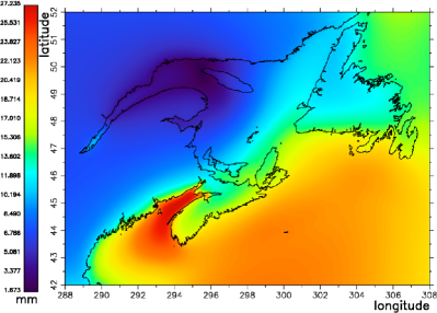
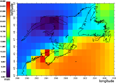
Figure 1: Mass loading caused by the $M_{2}$ ocean tide near Newfoundland island computed with two resolutions: $0.01^{\circ}\times 0.01^{\circ}$ grid (Left) and $1.0^{\circ}\times 1.0^{\circ}$ grid (Right)

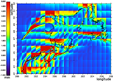
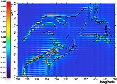
Figure 2: The difference of mass loading caused by the $M_{2}$ ocean tide computed with two resolutions: $1.0^{\circ}\times 1.0^{\circ}$ grid versus $0.01^{\circ}\times 0.01^{\circ}$ grid (Left) and $0.25^{\circ}\times 0.25^{\circ}$ grid versus $0.01^{\circ}\times 0.01^{\circ}$ grid (Left) and

Gridded loading at $1^{\circ}\times 1^{\circ}$ or $0.25^{\circ}\times 0.25^{\circ}$ resolutions should never be used for data reduction. The International Mass Loading Service computes loadings for 849 stations directly without the use of interpolation. This is sufficient for processing SLR, DORIS, and VLBI observations, since new stations are introduced infrequently. New GNSS stations are introduced much more frequently, and the situation when the GNSS station of interest is absent from the list of stations with pre-computed loading is more common. Figure 3 shows the Web interface that implements the on-demand loading computation. The on-demand computational procedure uses $V^{m}_{n}(t)$ and $H^{m}_{n}(t)$ coefficients that are evaluated and stored as soon as new data arrive. For this reason, the on-demand procedure is relatively quick: computation of loading displacements for 20 stations for a 1 year interval with the time step of 3 hours, in total 58,400 loading displacements, takes 20 minutes.

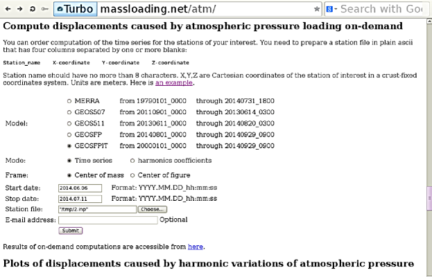
Figure 3: User interface to the on-demand computation of mass loading displacements

7 Conclusions and future work

At present, the International Mass Loading Service offers to the geodetic community computation of 3D displacements caused by the atmospheric pressure loading, land water storage loading, tidal and non-tidal ocean loading, free of charge, 24/7 with a latency from 8 hours (atmospheric and land water storage loading) to 30 days (non-tidal loading). The URL of the primary server is http://massloading.net, the URL of the secondary server is http://alt.massloading.net. The loading displacement were validated against the dataset of global VLBI observations for 2001–2014.

Further development: a) using weather forecast to 0–$24^{h}$ in the future. Latency will be eliminated. Accuracy degradation with respect to an assimilation model: 20% for the current instant; b) using OPeNDAP protocol for data distribution; c) automation of loading displacement ingestion: development of a client library that communicates with the loading servers automatically; d) generation of time series of the sum of all loadings on the fly with a user-requested time step; e) computing loading due to water level changes in lakes and big rivers.

This project was supported by NASA Earth Surface and Interior program, grant NNX12AQ29G.

References

- Carrere et al. (2012) Carrere L, Lyard F, Cancet M, Guillot A, Roblou L (2012) FES2012: A new global tidal model taking taking advantage of nearly 20 years of altimetry, Proceedings of meeting “20 Years of Altimetry”, Venice.
- Farrell (1972) Farrell, WE (1972) Deformation of the Earth by Surface Loads, Rev. Geophys. and Spac. Phys., vol. 10(3), 751–797
- Kalnay et al. (1996) Kalnay EM et al. (1996) Bull. Amer. Meteorol. Soc., 77, 437–471
- Molod et al. (2012) Molod A, Takacs L, Suarez M, Bacmeister J, Song I-S, Eichmann A (2012) The GEOS-5 Atmospheric General Circulation Model: Mean Climate and Development from MERRA to Fortuna, NASA/TM–2012, 104606, vol. 28
- Petrov and Boy (2004) Petrov L, Boy J-P (2004) Study of the atmospheric pressure loading signal in VLBI observations, JGR, 10.1029/2003JB002500, vol. 109, No. B03405.
- Ray (2013) Ray R (2013) Precise comparisons of bottom-pressure and altimetric ocean tides, JGR, 118, 4570–4584, doi:10.1002/jgrc.20336
- Reichle et al. (2011) Reichle RH, Koster RD, De Lannoy GJM, Forman BA, Liu Q, Mahanama SPP, Touré A (2011) J. Climate, 24, 6322–6338
- Rienecker, et al. (2008) Rienecker MM, et al. (2008) The GEOS Data Assimilation System — Documentation of Versions 5.0.1, 5.1.0, and 5.2.0, NASA/TM–2008–104606
- Rienecker, et al. (2011) Rienecker MM, et al. (2011) J. Climate, 24, 3624–3648
- Rodell et al. (2004) Rodell MP, et al (2004) The Global Land Data Assimilation System, Bull. Amer. Meteor. Soc., 85(3): 381–394
- Thomas (2002) Thomas M (2002) Ozeanisch induzierte Erdrotationsschwankungen, PhD