Topology Discovery for Linear Wireless Networks with Application to Train Backbone Inauguration

Abstract

A train backbone network consists of a sequence of nodes arranged in a linear topology. A key step that enables communication in such a network is that of topology discovery, or train inauguration, whereby nodes learn in a distributed fashion the physical topology of the backbone network. While the current standard for train inauguration assumes wired links between adjacent backbone nodes, this work investigates the more challenging scenario in which the nodes communicate wirelessly. The key motivations for this desired switch from wired topology discovery to wireless one are the flexibility and capability for expansion and upgrading of a wireless backbone. The implementation of topology discovery over wireless channels is made difficult by the broadcast nature of the wireless medium, and by fading and interference. A novel topology discovery protocol is proposed that overcomes these issues and requires relatively minor changes to the wired standard. The protocol is shown via analysis and numerical results to be robust to the impairments caused by the wireless channel including interference from other trains.

I Introduction

Wireless networks in which radio nodes are deployed according to a linear topology find numerous applications, including inter-vehicle communication systems [1]-[6] and train backbone communications [7], [8] (see Fig. 1). For such networks, it is convenient to have an automatic procedure that learns the network topology for any given configuration both at power-up time and in case nodes are added, replaced or removed during the network operation. For instance, the neighboring car in a train backbone is subject to change due to the fact that a single car or a group of cars of a train may be separated during the operation of shortening or lengthening a train. As a result, it is desirable that the system can learn the network topology when powered up and update any change in the topology as they occur without the intervention of a human operator. This is done via the process of topology discovery (TD).

The basic task of TD is to enable each node to learn the physical topology of the network. The physical topology consists of an ordered list of the media access control (MAC) addresses of the nodes in the network, where the order reflects the physical location of the nodes in the linear topology. According to current standards [8], the process operates via the exchange of MAC-level messages among the nodes in a distributive fashion. To illustrate the concept of a physical topology, an example is provided in Fig. 1 for a train backbone network. In this example, the physical topology lists the MAC addresses of the nodes, referred to as backbone nodes (BNs), in the order from 1 to 6.

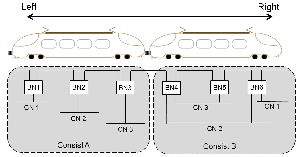
Figure 1: A wired backbone network with indicated physical and logical topologies. The physical topology refers to the ordering of the backbone nodes (BNs) and the logical topology means the ordering of the consist networks (CNs).

The TD protocol (TDP) [8] that is currently being standardized for train backbone communications applies to wired train backbone networks, in which the BNs are connected to their neighbors via dedicated wires. The TDP consists of two phases: 1) neighbor discovery: in this phase, each BN finds the MAC address of the neighboring BNs; 2) topology discovery: in this phase, the physical topology is detected via message exchange at the MAC layer. To implement TDP, the BNs transmit two types of MAC frames [8]: 1) hello frames, which carry only the MAC address of the sender BN and are used for neighbor discovery; and 2) topology frames, which carry information about the MAC addresses of the BNs currently “discovered” by the sender BN and are used for topology discovery.

While the standard [8] applies to wired backbone networks, there is high interest in the industry to develop a fully wireless solution. The key motivations for this desired switch from wired topology discovery to wireless one are the flexibility and the capability for expansion and upgrading of a wireless backbone. However, as it will be discussed, the wired TDP [8] does not lend itself to an implementation with wireless nodes. Moreover, any wireless implementation needs to contend with the inherently less reliable transmission medium. This work is hence devoted to developing a novel TDP, which will be referred to as wireless TDP (WTDP), that builds on the standard [8] but is suitable for implementation on a wireless backbone. Specifically, the aim of the proposed WTDP is to retain the main features of the wired counterpart TDP [8], while adapting messages and protocols to the new requirements for a wireless implementation.

The implementation of TDP [8] over a wireless network is made difficult by the broadcast nature of the wireless medium, and by fading and interference. Consider for instance the neighbor discovery phase. In wired TDP, hello frames are transmitted only to the neighbor(s) of a node as shown in Fig. 1. The neighbor discovery phase hence only requires that a single hello frame be received correctly from each neighbor. Wireless broadcasting instead, causes a frame to be received also by BNs that are not physical neighbors, making the detection of physical neighbors challenging [9]. This effect is compounded by the fact that, due to fading and interference, there is a non-zero probability that decoding errors impair the transmission from physical neighbors more significantly than the transmission from further nodes. Unlike the wired case, simultaneous transmissions in the same frequency band may lead to interference, which may cause the loss of a packet. For instance, with reference to Fig. 2, it is possible for BN 4 to decode the hello frame sent by BN 2 correctly, while decoding the hello frame from BN 3 incorrectly due to fading or interference. Another issue is that the standard [8] prescribes the multicasting of a topology frame to all the BNs in the network. In a wireless implementation, this is bound to create large backlogs and excessive interference. The proposed WTDP, detailed later in Sec. III, aims to address these challenges.

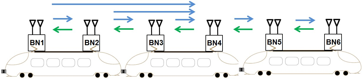
Figure 2: A wireless backbone network with indication of signals interfering the reception of BN 4.

We conclude this section with a remark on related work. Studies on wireless network topology discovery include [9]-[25] and references therein. In them, the key underlying assumption is that two nodes are considered to be neighbors if they are within their respective transmission ranges such that it is possible to establish a direct link between them. The topology discovery protocol hence aims at identifying connectivity, or reachability, properties of the network. This is typically done either by checking if a hello message is successfully received [9]-[19] or by measuring received signal strengths [20]-[25]. The design of specific topology discovery algorithms has been conducted in the context of different protocols such as IEEE 802.11, e.g., [16], or ZigBee [18]. Note that unlike the works in [26] and [27], wherein the inter-train and train-ground communication problems are addressed, this paper focuses on the problem of initializing the network for intra-train communication.

The topology discovery schemes that are available in the literature do not solve the problem of interest for the train backbone. The key distinguishing feature is that, in classical topology discovery, as discussed, a node is considered to be a neighbor as long as it is reached with a significantly large power. This goal is completely different from the requirements of train backbone inauguration, in which instead a neighbor is defined by its physical location and not by the strength of the received power. To see the difference, note that each backbone node has only two neighbors, one that should be specified as left-neighbor and one as right-neighbor. In contrast, a classical topology discovery scheme may identify an arbitrary number of neighbors that happen to receive the transmitted signal with sufficient power without consideration of their physical location. The approach proposed in this paper is meant to address the errors that can arise with conventional topology discovery schemes whereby physical neighbors may be incorrectly detected due to the fact that they receive a signal with sufficient strength.

The rest of the paper is organized as follows. In Sec. II, we review the TDP standard [8], while in Sec. III, we detail the proposed WTDP. In Sec. IV, we provide a performance analysis for the neighbor discovery phase of the proposed WTDP implemented with a slotted ALOHA MAC protocol. In Sec. V, we describe a case study consisting of two parallel trains. Numerical results of the proposed WTDP along with the performance analysis of neighbor discovery are presented in Sec. VI.

II Background: Wired Train Topology Discovery

In this section, we briefly review the standard wired TDP [8]. We observe that TD is also referred to as inauguration in [8]. Before the inauguration process, each BN knows its own MAC address and also the unique identifier (ID) of the consist networks (CNs) that are connected to the BN. A CN represents a subnetwork on the train. BNs may belong to multiple CNs, as illustrated in Fig. 1. The goal of TDP is to enable all the BNs to learn the physical and logical topologies of the train. As mentioned, the physical topology consists of an ordered list of BNs. The logical topology refers to an ordered list of CNs, with indication for each CN of the participant BNs, where the order reflects the physical location of the CNs. For instance, the logical topology for the network in Fig. 1 lists the CN IDs in the order A.1, A.2, A.3, B.3, B.2 and B.1, along with the corresponding MAC address of the BNs, as shown in Table. I. After inauguration, a BN ID is assigned to each BN according to the identified physical topology, and a subnet ID is assigned to each CN following the logical topology that is discovered. Taking the backbone network in Fig. 1 as an example, all six BNs are assigned with BN IDs in the ascending order from the left end to the right end, as illustrated in Table I. In the same order, the subnet IDs are assigned according to the logical topology (see [8] for further details).

Table I: Physical and logical topologies

CN ID	MAC address of connected BN	assigned BN ID	assigned subnet ID
A.1	BN 1’s MAC address	1	1
A.2	BN 2’s MAC address	2	2
A.3	BN 3’s MAC address	3	3
B.3	BN 4’s MAC address	4	4
B.3	BN 5’s MAC address	5	4
B.2	BN 4’s MAC address	4	5
B.2	BN 6’s MAC address	6	5
B.1	BN 6’s MAC address	6	6

Each BN, except the two at the beginning and end of the train, has two outgoing links, one toward its neighbor to the “right” and one towards the “left”. Note that the notions of “left” and “right” are common to all BNs on the backbone and are set by construction. Similarly, each BN has also two incoming links, one from the neighbor on the left and one from the neighbor on the right. As can be seen in Fig. 1, there are then an outgoing and an incoming link between a BN and a neighbor.

The BNs send two different types of frames, namely hello frames and topology frames. Both hello and topology frames are transmitted periodically and continuously. The hello frame contains the MAC address of the sender BN. This frame is sent only to the nodes’ neighbors. The topology frame instead contains information about the MAC addresses of previously discovered nodes. Specifically, the topology frame sent to the neighbor on the right contains an unordered list of all the currently known MAC address of the BNs on the left of the BN, and vice versa for the topology frame sent to the neighbor on the left. Topology frames are to be forwarded by the receiving BN in the same direction they have been received. This way, a topology frame is multicast to all BN in the given direction. As an example, in Fig. 1, if BN 4 has recognized BN 3 as a neighbor and has discovered that BNs 5 and 6 are on its right, the topology frame sent by BN 4 to BN 3 includes an unordered list of the MAC addresses of BNs 5 and 6. The topology frame also contains the IDs of the CNs that are connected to the sender BN, namely, CN B.3 and CN B.2 are connected to BN 4. After BN 3 receives this topology frame, the frame is forwarded to BN 2.

To summarize, the operation of TDP can be divided into two conceptually different phases, namely neighbor discovery and topology discovery.

• Neighbor discovery: Each BN receives hello frames from its incoming links to the left and/or to the right. Since each of these frames carries the MAC address of the sending neighbor, the BN at hand learns the MAC address of its neighbors after receiving one frame from the left and one from the right. The reception of these two frames completes the neighbor discovery phase.

• Topology discovery: Each BN keeps updated physical and logical topology tables (see Table I) based on the previously received hello and topology frames. As mentioned above, each transmitted topology frame to the left/right contains an unordered list of MAC addresses and the CN IDs that are connected to the sender BN. Upon reception of a topology frame, a BN updates its physical and logical topology tables. The BN can also check on whether its current tables coincide with the ones available at the BN that produced the topology frame thanks to a cyclic redundancy check (CRC) included in each topology frame.

Inauguration is declared to be complete by an operator that has access to the outcomes of the CRC steps carried out by the BNs.

III WTDP: Wireless Topology Discovery Protocol

As discussed in Sec. I, the wireless implementation of TDP poses significant technical challenges. To overcome these problems, the proposed WTDP prescribes a number of design choices at the deployment and protocol level as discussed in this section.

III-A Deployment

WTDP is based on a physical implementation of the system that leverages directional antennas and frequency planning.

• Directional antenna: All the BNs have two directional antennas and share the notion of a “left” and a “right” direction. Each BN hence can transmit and receive on both its right-pointing and left-pointing antennas. Note that the assumption concerning the common notion of the left and right directions is consistent with the model considered in the wired standard [8]. Directional antennas enable a BN to distinguish between the signals received from the left and right directions.

• Frequency planning: To cope with interference, two sets of frequencies are used, one for the right-pointing antennas and one for the left-pointing antennas. Each directional antenna operates on two different frequencies, one for transmission and one for reception. Moreover, the same frequency is reused every $F$ hops. Therefore, if $F=1$, we have full frequency reuse in each direction; instead, if $F>1$, there are $F-1$ BNs transmitting in the same direction but using different frequencies between two transmitters using the same frequency. We refer to Fig. 3 for an illustration. Note that, with a frequency reuse $1/F$, the closest non-neighboring BN that may receive a hello frame is $F-1$ hops away. A more conservative frequency reuse hence reduces the danger of receiving a hello frame from a non-neighboring BN. A smaller frequency reuse also reduces the effect of interference.

  

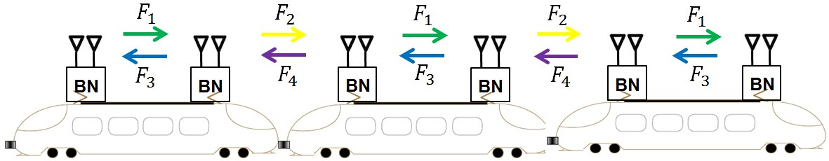
  Figure 3: Illustration of the proposed physical implementation of WTDP with directional antenna and frequency planning with $F=2$. $F_{i}$ indicates the $i$th available carrier frequency.

III-B The Proposed Protocol

In this section, we detail the operation of the proposed WTDP. The proposed WTDP prescribes each BN to operate according to the high-level flowchart of Fig. 4, which is further detailed in Fig. 5. As shown in Figs. 4 and 5, the proposed WTDP includes five phases: I. Neighbor discovery; II. Pairwise consistency check (PCC); III. Neighbor discovery failure check; IV. Topology discovery; and V. Topology convergency check. We first explain the flow of these phases with reference to Fig. 4. We then detail the steps of the algorithm in the following subsections.

III-B1 Overview

At first, each BN attempts to identify a neighbor during the neighbor discovery phase (I). If a neighbor is identified, then, in order to correct some of the possible errors of neighbor discovery errors, the BN performs the PCC (II). If the identified neighbor passes the PCC, it is upgraded to a locked neighbor; otherwise the identified neighbor is discarded and neighbor discovery needs to be restarted. After an identified neighbor is established, the BN also starts the neighbor discovery failure check phase (III). Whenever a neighbor discovery failure is detected, a “red flag” is raised. Upon the observation of a red flag, the operator, which is informed about “green flags” or “red flags” raised by the BNs, should restart the inauguration process. Once a locked neighbor is established, the topology discovery phase (IV) starts. The completion of the topology discovery phase for each BN is indicated by the BN via a raised “green flag”, which signals that the topology convergency check (V) is passed.

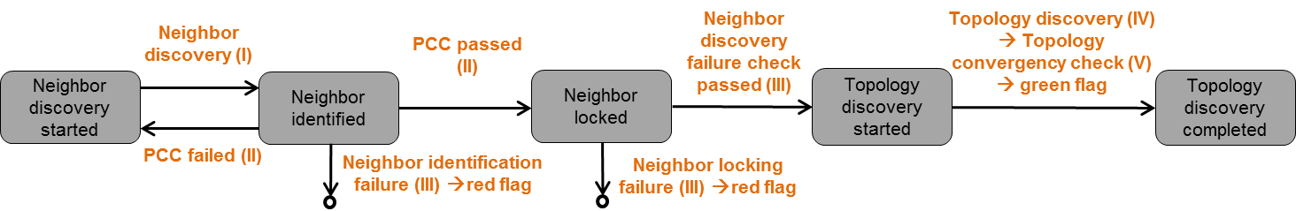
Figure 4: A high-level illustration of the operation of a BN in the proposed WTDP. The circle indicates that a red flag has been raised and that the BN is waiting for the inauguration process to be restarted.

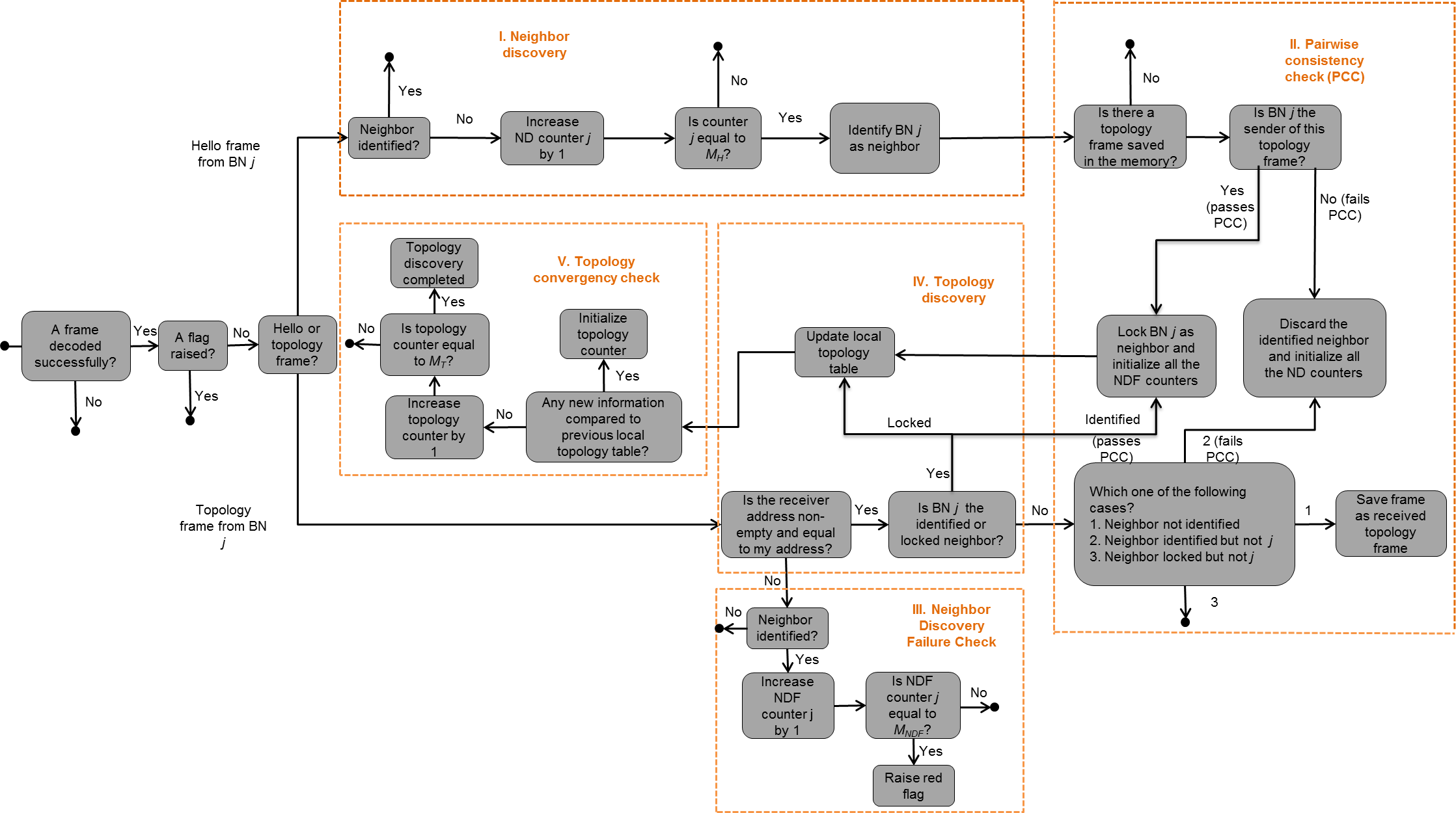
Figure 5: Illustration of the operation of a BN in the proposed WTDP. The black dot means that the BN is ready to process the next frame.

III-B2 Data Structures

Each BN stores and updates the following data structures, whose use will be detailed in the next subsections.

• Neighbor discovery (ND) counters: a list of neighbor discovery counters, one for each of the BNs from which the BN has received a hello frame;

• Topology table: an ordered list of the MAC addresses of the discovered BNs, where the order reflects the physical location of the BNs;

• Topology counter: a counter that accounts for the current number of consecutive times that a topology frame has been received but the local topology table has not been changed;

• Neighbor discovery failure (NDF) check counters: a list of counters, one for each of the BNs from which a topology frame addressed to any other BN has been received.

III-B3 Neighbor Discovery

As discussed in Sec. I, neighbor discovery in a wireless train backbone is significantly more complex than in the wired counterpart system. This is due to the broadcast properties of the wireless channel, which cause the hello frame transmitted by a BN to be received not only by the actual neighbor BN but generally also by further away BNs. As a result, unlike in the wired system, reception of the hello frame does not, per se, establish that the sender BN is a neighbor.

In order to achieve neighbor discovery, the proposed scheme leverages the fact that, on the average, the power received from an actual neighboring BN is larger than that received from any other BN. This is due to the lower path loss between closer nodes. Therefore, for instance, it is more likely that a hello frame is received correctly from an actual neighbor than from farther BNs. It is critical to note, however, that, due to fading, it cannot be excluded that a hello frame from a non-neighboring BN is received successfully, while that of the actual neighbor is not.

Based on the discussion above, we propose the following simple neighbor discovery algorithm. For each hello frame correctly decoded in either direction, if the MAC of the sender BN is already in the list of ND counters, then the corresponding counter is increased by one; else, a new counter is created, initialized to zero and associated to the MAC address at hand. A node is identified to be a neighbor if it is the first whose ND counter reaches a pre-defined threshold $M_{H}$. In this event, this node is defined as the identified neighbor of the receiving BN. The described operations are within in the “neighbor discovery” block of Fig. 5.

We remark that the simple algorithm proposed above makes exclusive use of information available at the MAC layer, namely the number of successfully received frames from different MAC addresses. This choice has been made in order to allow for a simpler implementation, and is in line with the wired counterpart standard.

III-B4 Pairwise Consistency Check (PCC)

In order to reduce the probability of incorrect neighbor discovery, we propose to perform a pairwise consistency check (PCC) upon the reception of a topology frame. The key observation is that the topology frame is addressed to the currently identified neighbor. Note that the hello frames are instead broadcast. Therefore, based on the reception of topology frames, each BN can verify whether the neighbor discovery is pairwise consistent with respect to its neighbor in either direction. By pairwise consistency, we mean that two BNs consider each other as neighbors, one on the left and the other on the right. If a topology frame is received from a BN that is not considered as a neighbor, then the receiving BN can conclude that neighbor discovery is not pairwise consistent in the direction of the received packet.

To be specific, if the topology frame is received from the currently identified neighbor, this identified neighbor passes the PCC and is upgraded to the status of locked neighbor. Once a locked neighbor is established for a BN, any received topology frame from other BNs is discarded. Instead, if a BN receives a topology frame from a BN different from the identified neighbor, its identified neighbor fails the PCC and all ND counters are reinitialized to zero in order to restart the neighbor discovery phase for the receiving BN. Note that, if a topology frame is received before any identified neighbor is established, the frame will be saved for a PCC later. The detailed procedure for PCC is described within the “pairwise consistency check” block of Fig. 5.

III-B5 Neighbor Discovery Failure Check

PCC helps improve the accuracy of neighbor discovery, but it does not rectify errors that occur when two neighboring BNs identify their neighbors incorrectly. This type of failure is defined as neighbor identification failure. An example is shown in Fig. 6. It is seen that, if BN 3 identifies BN 5 as a neighbor and BN 4 identifies BN 2 as a neighbor, this error cannot be corrected by PCC because neither BN 3 nor BN 4 will send a topology frame to the other.

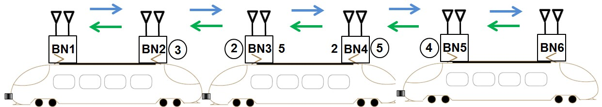
Figure 6: An example of neighbor identification failure. A number on the left/right of each BN refers to identified neighbors on the left/right of the BN. A circled numbers means a neighbor has been locked.

In order to identify the neighbor discovery failure described above, we propose to perform neighbor discovery failure check. The idea is that, after a neighbor has been identified but not locked, if a BN receives too many topology frames addressed to a BN other than itself, it is probable that its actual neighbor had identified some other BN as its neighbor. In this case, this BN cannot successfully complete neighbor discovery and a red flag is raised. Specifically, each BN maintains an NDF counter, which counts the number of topology frames addressed to other BNs that are received after a neighbor has been identified. When the NDF counter reaches a pre-defined threshold $M_{NDF}$, the BN raises a red flag warning the train operator of a neighbor discovery failure.

The other possible neighbor discovery failure happens when a BN is established as the locked neighbors by more than one BN. This causes the problem that certain BNs do not receive topology frame from their locked neighbors and thus topology discovery will never be completed. We define this type of failure as neighbor locking failure. An example is shown in Fig. 7, where although BN 2 established BN 4 as its locked neighbor, BN 4 has locked with BN 3, and hence no topology frames will be received by BN 2 from BN 4. To deal with this problem, after the neighbor of a BN is locked, the NDF counter is initialized and used to count topology frames received from BNs different from its locked neighbor. A red flag is raised if the NDF counter exceeds the threshold.

We remark that due to the introduction of the phase II (PCC) and phase III (neighbor discovery failure check), the proposed protocol is a bidirectional protocol. Hence, these phases can also be used to counteract hello flooding attacks based on wormhole (tunneling) [30], [31], or compromised nodes [32], [33].

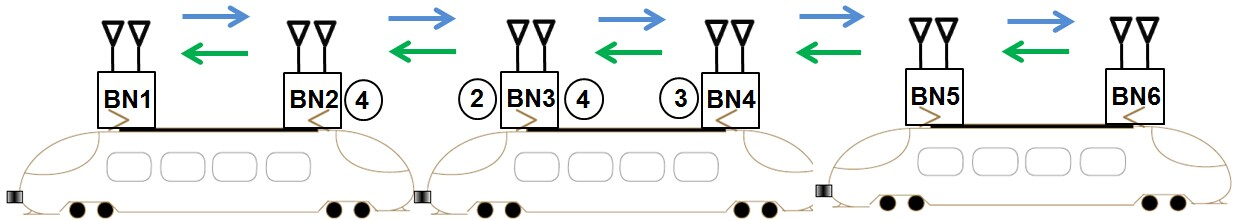
Figure 7: An example of neighbor locking failure. A circled number on the left/right of each BN refers to a locked neighbor on the left/right of the BN.

III-B6 Topology Discovery

As described in Sec. I, multicasting a topology frame is impractical in WTDP. To solve this issue, we propose that, in WTDP, the topology frame contains an ordered, rather than an unordered as in wired TDP, list of MAC addresses in the current topology table of the sender node. Specifically, the topology frame sent to the neighbor on the right contains all the currently known MAC address of the BNs on the left of the BN in the discovered physical order, and vice versa for the topology frame sent to the neighbor on the left. The topology frame also includes the CN IDs that are connected to, rather than only the sender BN as in wired TDP, all BNs currently discovered. Taking the wireless backbone network in Fig. 2 as an example, if the associated logical topology is identical to that shown in Fig. 1, and if BN 4 has identified BN 3 as a neighbor and has discovered that BNs 5 and 6 are on its right, the topology frame sent by BN 4 to BN 3 contains an ordered list of MAC addresses of BNs 5 and 6. It also includes the IDs of the CNs that are connected to the BNs 4, 5 and 6, namely, CN B.3 and CN B.2 are connected to BN 4; CN B.3 is connected to BN 5; CN B.2 and CN B.1 are connected to BN 6. A topology frame is sent to an identified or locked neighbor. Based on a received topology frame, the receiving BN updates its local topology table only if the received topology frame is from its locked neighbor. Note that after the physical topology is learned, the logical topology can be learned in the same way as in the wired TDP (see [8] for details). Therefore, we focus on the physical topology discovery for WTDP next.

After a successful neighbor discovery has been resolved for all BNs, it is necessary and sufficient to have a “right-ward” and a “left-ward” pass in order to complete topology discovery. For instance, in Fig. 2, assume that the protocol starts from BN 1, which sends a topology frame to its neighbor on the right BN 2, which in turn sends a topology frame to its neighbor BN 3, and so on until BN 6. At the end of this right-ward pass, it is easy to see that each BN in Fig. 2 learns the backbone topology on its right. A similar left-ward pass completes the topology discovery at each BN. It can also be seen that the mentioned frames are also necessary in order to learn the train topology.

We emphasize that the proposed WTDP differs from the standard wired TDP in that the latter prescribes multicasting of topology frames and the inclusion of an unordered list of discovered nodes and the CN IDs that are connected to the sender BN only in the topology frames. The operation of the topology discovery phase is described by the functions enclosed in the “topology discovery” block of Fig. 5.

III-B7 Topology Convergency Check

In order for the operator to make a decision about the completion of the inauguration process, the BNs must report on the status of their topology discovery phase. To this end, each BN runs a topology convergence check as shown in the “topology convergency check” block of Fig. 5. Accordingly, when a topology frame is received from a locked neighbor, if any change needs to be made to the local topology table, the topology counter for the BN is initialized; otherwise, the counter is increased by one. The topology discovery completion for a BN is claimed if the topology counter reaches a pre-defined threshold $M_{T}$. In other words, the topology discovery is considered to be complete by a BN if no change is made to its topology frame across $M_{T}$ successively received topology frames from the locked neighbor. The completion of topology discovery is indicated by green flags raised by the BNs.

IV Performance Analysis

In order to get some insights into the performance of the proposed WTDP, we consider the implementation of WTDP with a slotted ALOHA MAC protocol. Note that the protocol does not depend on the adoption of a specific MAC layer protocol and that slotted ALOHA is assumed here to enable analysis. According to slotted ALOHA, time is slotted, a transmitted frame takes one slot, and each BN transmits a frame in a slot with probability $p$. Specifically, at each time slot, a BN transmits a hello frame with probability $p_{H}$, and transmits a topology frame with probability $p_{T}$. Hence, the transmission probability $p$ is the sum of $p_{H}$ and $p_{T}$, i.e., $p=p_{H}+p_{T}$.

Flat Rayleigh fading channels are assumed such that the instantaneous channel gain between two nodes $k$ hops away can be written as $\mathrm{SNR_{0}}\left|h\right|^{2}/(1+(k-1)F)^{\eta}$, where we define the average signal to noise ratio (SNR) for two nodes one hop away as $\mathrm{SN}\mathrm{R}_{0}$, $|h|^{2}$ is exponentially distributed with mean one, and $\eta$ denotes the path loss exponent. Furthermore, the channels across different time slots are assumed to be independent, while the channel is a constant within the period of a frame transmission. We note that a more general channel model, such as Rician or Nakagami fading, could also be accommodated in the analysis but at the cost of a more cumbersome notation due to the lack of some closed-form expressions that are available for Rayleigh fading as discussed below. We present experiments with Rician fading in Sec. VI.

In the following, we provide an analysis for the neighbor discovery phase in terms of the probability of correct neighbor discovery and of the average time required to complete neighbor discovery. There two conflicting criteria will also be combined to yield the average time needed to achieve successful neighbor discovery. The goal of the analysis is to obtain insights into the selection of the critical threshold parameter $M_{H}$. The performance of the overall WTDP will be evaluated in the next section via numerical results.

IV-A Neighbor Discovery for a Single BN

In this subsection, we consider the neighbor discovery for a single receiving BN on any given side. We compute the probability $Q_{C,ND}$ of correct neighbor discovery and the cumulative distribution function (CDF) $F_{T_{ND}}\left(t\right)$ of the time $T_{ND}$ that it takes to complete neighbor discovery.

To elaborate, assume that the furthest BN from which hello frames can be received is $K$ hops away. The signal-to-interference-and-noise ratio (SINR) for the signal transmitted by a BN $k$ hops away is given by

$$\mathrm{SIN}\mathrm{R}_{k}=\frac{\left|h_{k}\right|^{2}\frac{\textrm{$\mathrm{SNR_{0}}$}}{(1+(k-1)F)^{\eta}}}{1+\sum_{k^{\prime}\neq k}^{K}i_{k^{\prime}}\left|h_{k^{\prime}}\right|^{2}\frac{\textrm{$\mathrm{SNR}_{0}$}}{(1+(k^{\prime}-1)F)^{\eta}}},$$ (1)

where $i_{k^{\prime}}=1$ if the BN $k^{\prime}$ hops away is transmitting and $i_{k^{\prime}}=0$ otherwise. Moreover, the instantaneous channel capacity for the link between the two nodes, which are $k$ hops away from each other, is given by [34]

$$C_{k}=\log\left(1+\mathrm{SINR}_{k}\right).$$ (2)

Whenever the transmission rate $\mathrm{\mathit{R\,}[bits/sec/Hz]}$ is not larger than the instantaneous capacity $C_{k}$, the packet transmitted by the BN $k$ hops away is correctly received, and an outage is declared otherwise [35].

Define the vector $\mathbf{i}=[i_{1},\cdots,i_{K}]^{T}$ that defines the set of currently transmitting BNs. At any time slot, the probability of a successful frame reception from a node $k$ hops away conditioned on $\mathbf{i}$ can be expressed as

$$Q{}_{S}(k|\mathbf{i})=i_{k}\frac{p_{H}}{p}\Pr\left[C_{k}\geq R|\mathbf{i}\right].$$ (3)

Substituting (2) into (3) leads to

$$Q{}_{S}(k|\mathbf{i}) =i_{k}\frac{p_{H}}{p}\Pr\Bigg{[}\frac{|h_{k}|^{2}\mathrm{SNR_{0}}}{(1+(k-1)F)^{\eta}}\geq$$

$$2^{R}-1+\sum_{k^{\prime}\neq k}^{K}i_{k^{\prime}}(2^{R}-1)\mathrm{\frac{\mbox{$|h_{k^{\prime}}|^{2}$}SNR_{0}}{(\mbox{$1+(k^{\prime}-1)F$})^{\eta}}\Bigg{]}}.$$ (4)

Using the result in [36], we get

$$Q{}_{S}(k|\mathbf{i})= i_{k}\frac{p_{H}}{p}\exp\left(-\frac{2^{R}-1}{\mathrm{SNR_{0}}}(1+(k-1)F)^{\eta}\right)$$

$$\times \prod_{k^{\prime}\neq k}^{K}\left(\frac{1}{1+i_{k^{\prime}}(2^{R}-1)\frac{(1+(k-1)F)^{\eta}}{(\mbox{$1+(k^{\prime}-1)F$})^{\eta}}}\right).$$ (5)

Averaging over all possible transmission states $\mathbf{i}$, we can write the probability of a successful frame transmission from a node $k$ hops away as

$$Q{}_{S}(k)=\sum_{\mathbf{i}\in\mathbf{\mathbf{\mathcal{I}}}}P_{\boldsymbol{\mathbf{i}}}\left(\mathbf{i}\right)Q{}_{S}(k|\mathbf{i}),$$ (6)

where $\mathbf{\mathcal{I}}$ denotes the set that contains all possible $2^{K}$ transmission state vectors and $P_{\mathbf{\mathbf{i}}}\left(\mathbf{i}\right)$ is the probability mass function of vector $\mathbf{\mathbf{i}}$.

Due to the independence of the fading channels across the time slots, the time $T_{k}$ that it takes to receive $M_{H}$ hello frames from a BN $k$ hops away is distributed as $T_{k}\sim NB(M_{H},Q_{S}(k))$, where we use the notation $NB(M,p)$ to denote a negative binomial distribution with parameter $(M,p)$. Accordingly, the probability mass function of $T_{k}$ is given by [37]

$$P_{T_{k}}\left(t\right)=\left(\begin{array}[]{c}t-1\\ M_{H}-1\end{array}\right)Q_{S}(k)^{M_{H}}(1-Q_{S}\left(k\right))^{t-M_{H}},$$ (7)

for $t\geq M_{H}$; and the complementary cumulative distribution function (CCDF) of $T_{k}$, which equals to the probability that hello frames sent by a BN $k$ hops away are received successfully $M_{H}$ times after the $t$th time slot, can be expressed as [37]

$$\bar{F}_{T_{k}}(t)=1-I_{Q_{S}(k)}(M_{H},t-M_{H}+1)\textrm{, for $t\geq M_{H}$}.$$ (8)

where $I_{x}(z,w)$ denotes the regularized incomplete beta function with parameters ($x,z,w$).

So far, we have considered the distribution of the time needed to receive $M_{H}$ hello frames from a given transmitting BN. We are now interested in deriving the probability $Q_{C,ND}$ of correct neighbor discovery. This calculation is complicated by the fact that the receptions of frames from different BNs are correlated with each other due to the mutual interference among BNs. To address this issue, we make here the approximation that the decoding outcomes for the packets sent by different BNs are independent. The validity of this approximation will be evaluated in Sec. VI by numerical results. Recall that, if the first BN from which hello frames are received successfully $M_{H}$ times is the BN one hop away, neighbor discovery is correct. Hence, using the said independence assumption, the probability of correct neighbor discovery for a single receiving BN is

$$Q_{C,ND}=\sum_{t\geq M_{H}}^{\infty}\left[P_{T_{1}}\left(t\right)\prod_{k\geq 2}^{K}\bar{F}_{T_{k}}(t)\right].$$ (9)

Finally, regardless of whether it is correct or not, neighbor discovery is considered to be complete when a BN decodes $M_{H}$ hello frames successfully from at least one of other transmitting BNs. The CDF of the time it takes to complete neighbor discovery for the BN $T_{ND}$ can be expressed, under the independence assumption, as

$$F_{T_{ND}}\left(t\right) =1-\Pr\left[T_{ND}>t\right]$$

$$=1-\Pr\left[\mathrm{\min}\left\{T_{1},T_{2}...,T_{K}\right\}>t\right]$$

$$=1-\prod_{k=1}^{K}\bar{F}_{T_{k}}(t).$$ (10)

IV-B Neighbor Discovery Across the Entire Network

In this subsection, we derive the performance metrics of neighbor discovery across the entire network. Specifically, we derive the probability $Q_{C,ND}^{*}$ of correct neighbor discovery, the average time $E[T_{ND}^{*}]$ required to complete neighbor discovery for all nodes and the average time $E[T_{ND,\mathrm{\mathit{suc}}}^{*}]$ needed to achieve a successful neighbor discovery.

Because the neighbor discovery outcomes for different BNs are not independent, the analytical derivation of statistical quantities associated with neighbor discovery performance is challenging. For this reason, we will make the approximation mentioned above that the neighbor discovery outcomes for different BNs are independent. With this approximation, probability of correct left and right neighbor discovery for all BNs in the network can be expressed as

$$Q_{C,ND}^{*}=\left(Q_{C,ND}\right)^{2D},$$ (11)

where $D$ denotes the total number of receiving BNs and the factor $2$ stems from the fact that different frequencies are used for transmission and reception and hence, the left neighbor discovery is independent from the right neighbor discovery. Similarly, the CDF of the time it takes to achieve a successful neighbor discovery on both left and right sides is given by

$$F_{T_{ND,L}^{*}}\left(t\right) =\left(F_{T_{ND,L}}\left(t\right)\right)^{2D}.$$ (12)

The average time needed to achieve a successful neighbor discovery $E[T_{ND}^{*}]$ is then given by

$$E\left[T_{ND}^{*}\right]=\sum_{t=0}^{\infty}\left[1-F_{T_{ND}^{*}}(t)\right].$$ (13)

Next we combine the two statistical quantities $Q_{C,ND}^{*}$ and $E\left[T_{ND}^{*}\right]$ to yield the average time it takes to achieve a successful neighbor discovery $E[T_{ND,\mathrm{\mathit{suc}}}^{*}]$. Using Wald’s equality [38], this can be evaluated as the ratio

$$E[T_{ND,suc}^{*}]=\frac{E\left[T_{ND}^{*}\right]}{Q_{C,ND}^{*}}.$$ (14)

V Case Study: Trains on Parallel Tracks

In this section, we describe a scenario of practical interest in which two trains located on parallel tracks perform separate inauguration processes. This set-up will be further elaborated on in Sec. VI via numerical results. As shown in Fig. 8, we assume the same number of BNs for each train, and we denote the distance between a BN and its neighbor on the same train as $\Delta$, while $l$ denotes the distance between two trains. We also assume that BNs are aligned as in Fig. 8. Let the directional antenna of each BN have a mainbeam of width $\theta$, while sidelobes have a $L$ dB loss compared to the mainlobe. For instance, in Fig. 8, BN 3 and BN 4 on train 2 are in the side lobe region of the right-pointing antenna of BN 3 on train 1, and hence are received by BN 3 on train 1 with a loss of $L$ dB. Instead, no loss occurs for the reception by BN 3 on train 1 of the signals sent by BN 5 and BN 6 on train 2 or BNs 4-6 on train 1.

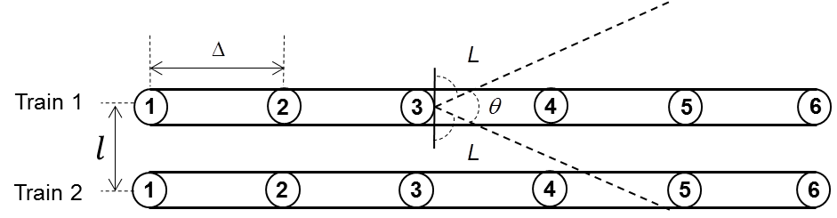
Figure 8: An example of two trains on parallel tracks (top view). Also shown is the antenna gain pattern for BN 3 on train 1.

VI Numerical Results and Discussions

In this section, we evaluate the performance of the proposed WTDP as applied to a wireless network that runs the ALOHA MAC protocol. Unless stated otherwise, we assume the following conditions: i) a flat Rayleigh fading channels as described in Sec. IV; ii) a path loss exponent $\eta=3.5$; iii) an average SNR of $15\,\mathrm{dB}$ for two nodes one hop away, i.e., $\mathrm{SN}\mathrm{R}_{0}=15\,\mathrm{dB}$; iv) a total of six BNs in the network; v) at any time slot, a hello frame is transmitted with probability, $p_{H}=0.15$, and a topology frame is transmitted with probability, $p_{T}=0.15$; vi) a data rate $R$ $1.5\,\mathrm{bits/sec/Hz}$ for the hello frames, and vii) full frequency reuse is adopted, i.e., $F=1$. We recall that a more conservative frequency reuse would alleviate interference and therefore improve the performance.

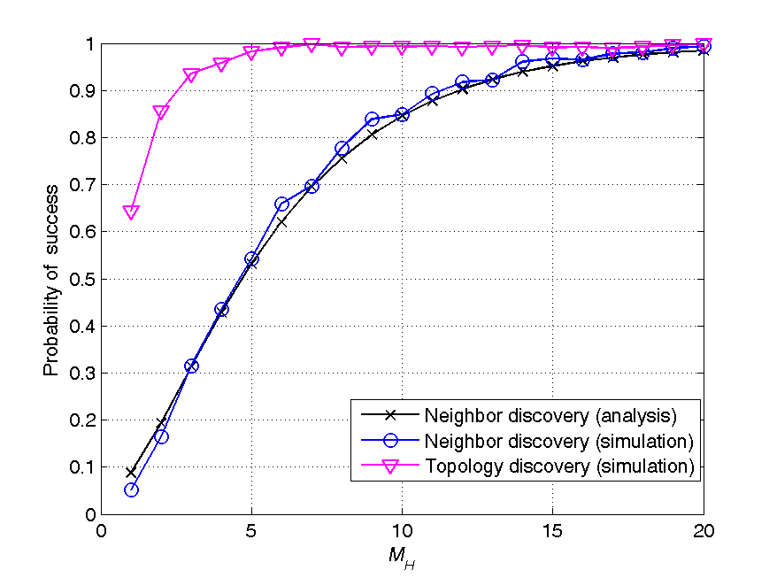
Figure 9: The probability of success of neighbor discovery and of overall inauguration process versus the threshold $M_{H}$ used for neighbor discovery ($p_{H}=0.15$, $p_{T}=0.15$ and $\mathrm{SN}\mathrm{R}_{0}=15\,\mathrm{dB}$).

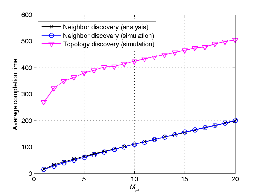
Figure 10: The average time required to complete neighbor discovery and to complete the entire inauguration process versus $M_{H}$ ($p_{H}=0.15$, $p_{T}=0.15$ and $\mathrm{SN}\mathrm{R}_{0}=15\,\mathrm{dB}$).

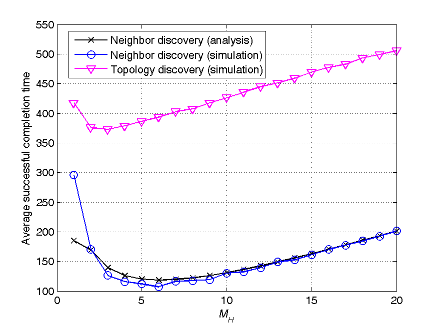
Figure 11: The average time needed to achieve a successful neighbor discovery and overall inauguration versus $M_{H}$ ($p_{H}=0.15$, $p_{T}=0.15$ and $\mathrm{SN}\mathrm{R}_{0}=15\,\mathrm{dB}$).

VI-A Effects of the Threshold $M_{H}$

We first investigate the effect of the threshold parameter $M_{H}$ on the neighbor discovery performance. This discussion is also meant to corroborate the validity of the analysis in Sec. IV. In Figs. 9-11, the probability of correct neighbor discovery, the average time required to complete neighbor discovery and the average time needed to achieve a successful neighbor discovery are shown as a function of $M_{H}$, respectively. We plot both the analytical results (11), (13) and (14) and the performance obtained via Monte Carlo simulations. It can be seen from Figs. 9-11, that the analysis predicts the performance of neighbor discovery well in terms of the three criteria. As expected, the success rate and time needed to complete neighbor discovery increase as threshold $M_{H}$ increases. This leads to a trade-off in the selection of $M_{H}$: a larger $M_{H}$ improves the probability of successful neighbor discovery but, at the same time, it increases the time needed for neighbor discovery. This trade-off is illustrated in Fig. 11, which demonstrates that there exists a value of $M_{H}$ that minimizes the time needed to achieve successful neighbor discovery. We observe that the analysis allows to correctly predict the optimal value of $M_{H}$.

In Figs. 9-11, the performance for the overall proposed inauguration process including all the phases described in Sec. III is also presented. To this end, we set $M_{NDF}=20$ and $M_{T}=30$ and evaluate the performance via Monte Carlo simulations. The dramatic success rate improvement for the inauguration over neighbor discovery is to be ascribed to the PCC. This improvement can be also seen to decrease the optimal value of $M_{H}$. It can also be observed that there is a difference of about 300 time slots between the time required to complete neighbor discovery and the time required to complete the whole inauguration process. This is due to the fact that besides neighbor discovery, the inauguration process needs to complete also topology discovery.

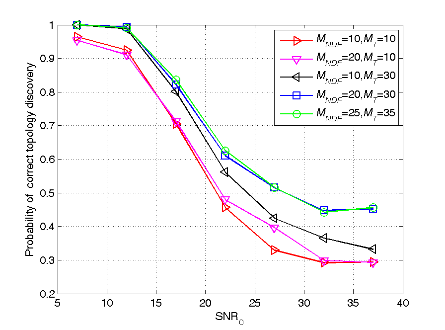
Figure 12: The probability of successful topology discovery versus $\mathrm{SN}\mathrm{R}_{0}$ for different values of the thresholds $M_{NDF}$ and $M_{T}$ ($p_{H}=0.15$, $p_{T}=0.15$ and $M_{H}=3$).

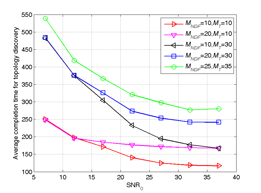
Figure 13: The average time required to complete topology discovery vs. $\mathrm{SNR}_{0}$ for different values of the thresholds $M_{NDF}$ and $M_{T}$ ($p_{H}=0.15$, $p_{T}=0.15$ and $M_{H}=3$).

VI-B Effects of Thresholds $M_{NDF}$ and $M_{T}$

We now explore the effects of two thresholds $M_{NDF}$ and $M_{T}$ on the performance of WTDP. The value of threshold $M_{H}$ is set to 3 based on the discussion above. In Fig. 12, we plot the probabilities of correct topology discovery and in Fig. 13 we show the average time required to complete topology discovery versus the average one-hop SNR, parameterized by different values of $M_{NDF}$ and $M_{T}$. It can be seen that larger thresholds $M_{NDF}$ and $M_{T}$ result in an improved probability of correct topology discovery. This is because it is more unlikely that an incorrect identification of neighbor discovery failure occurs with a larger $M_{NDF}$ (see Sec. III-B5) while a larger $M_{T}$ tends to improve the efficiency of the topology convergency check (see Sec. III-B7). On the flip side, Fig. 13 shows that larger values of $M_{NDF}$ and $M_{T}$ always lead to longer average time needed to complete the inauguration.

VI-C Neighbor Discovery Over Rician Fading Channels

We now consider neighbor discovery over flat-fading Rician channels. We recall that the defining parameter of Rician fading is the $K$-factor, which is defined as the power ratio of the line-of-sight component and diffuse components [39]. In Fig. 14, we present the probability of correct neighbor discovery versus the Rician $K$-factor with different values of the transmission probability $p$ and of the train speed $v$. We adopt the standard Jakes model [39] to account for channel correlation as a function of the train velocity v. We set the threshold for neighbor discovery to $M_{H}=10$ and equal probability for transmission of a hello and a topology frames. It can be seen from Fig. 14 that in the low-$K$ regime, the success rate is low over static channels, i.e. $v=0\,\mathrm{km/hour}$, but a minor increase in the train speed, i.e., with $v=1\,\mathrm{km/hour}$, significantly improves the success rate. This is because with static channels, time diversity is lost, but due to the long duration of a time slot ($T=100\,\mathrm{ms}$), a speed as low as $1\,\mathrm{km/hour}$ results in uncorrelated channel gains across different time slots. This can be verified by the fact that the success rate with low $K$-factor at the speed of $1\,\mathrm{km/hour}$ (see Fig. 14) converges to the success rate of 86%, which is also the success rate for neighbor discovery with the threshold $M_{H}=10$ shown in Fig. 9. Instead, in high-$K$ regime, a larger transmission probability $p$ results in higher probability correct neighbor discovery in the static case. This is explained by the fact that in this regime, the channel gain tends to be dominant by the line-of-sight component, yielding successful frame transmissions from both neighboring BNs and non-neighboring BNs in absence of collision. A larger transmission probability results in more collisions, which in turn reduce the chance of successful frame decoding, more severely for frames sent by non-neighboring BNs than for the ones sent by neighboring BNs, since the latter BNs are received with sufficient power not to incur outage.

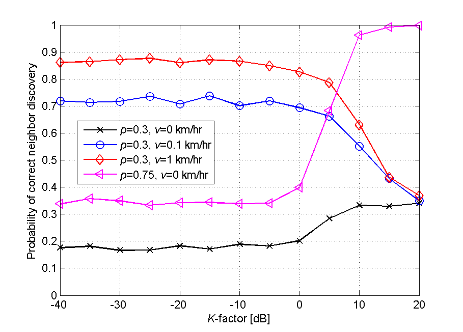
Figure 14: The probability of successful neighbor discovery versus the $K$-factor for Rician fading channels with different values of train speeds and the transmission probabilities ($M_{H}=10$ and $\mathrm{SNR}_{0}=15\,\mathrm{dB}$).

VI-D Neighbor Discovery of Two Parallel Trains

In this subsection, we evaluate the neighbor discovery performance with two trains located on parallel tracks as described in Sec. V. The BNs of both trains transmit by using the slotted ALOHA protocol as per Sec. IV. Note that while this assumes synchronization between the trains, we expect the effect of inter-train interference to be qualitatively the same even under asynchronous MACs. We evaluate the neighbor discovery performance for train 1 with train 2 serving as interference. Each train is equipped with six BNs. The beam width $\theta$ is selected as $\theta=\pi/3$. Rayleigh fading is assumed.

In Figs. 15 and 16, we show the probability of correct neighbor discovery and the average time needed to complete neighbor discovery versus the ratio $l/\Delta$, parameterized by sidelobe attenuation $L=6\,\mathrm{d\mathrm{B}}$ and $L=12\,\mathrm{dB}$. Also shown for reference is the performance for the case in which only train 1 is present, i.e., no inter-train interference exists. It can be seen from Fig. 15 that the accuracy of neighbor discovery is poor for small $l/\Delta$, and that, as the ratio $l/\Delta$ increases, the probability of successful neighbor discovery first increases and then decreases, reaching the interference-free performance for $l/\Delta$ large enough. This can be explained as follows. With small $l/\Delta$, the BNs on train 2 tend to be selected by the neighbor discovery process run at BNs on train 1, causing the failure of neighbor discovery. This effect becomes less pronounced as the ratio $l/\Delta$ increases and hence the performance is enhanced. Interestingly, for values of $l/\Delta$ close to one, the interference may be even beneficial to neighbor discovery. The reason for this is similar to the one for the scenario in which concurrent transmission happens with a single train (see Sec. VI-C). It is also seen that a larger sidelobe attenuation causes this effect to be observed for lower values of $l/\Delta$. As $l/\Delta$ increases further, the performance converges to that of a single train with no interference.

In contrast to the probability of correct neighbor discovery, the average time required to complete neighbor discovery is shown in Fig. 16 to be first degraded as $l/\Delta$ increases before finally converging to the interference-free performance. This is because when $l/\Delta$ is close to one, frames from both trains tend to be received with similar powers leading to numerous outage events. Instead, if $l/\Delta$ is smaller, the BNs on train 1 will more likely choose BNs on train 2 as neighbors, while for larger $l/\Delta$, neighbors tends to be successful.

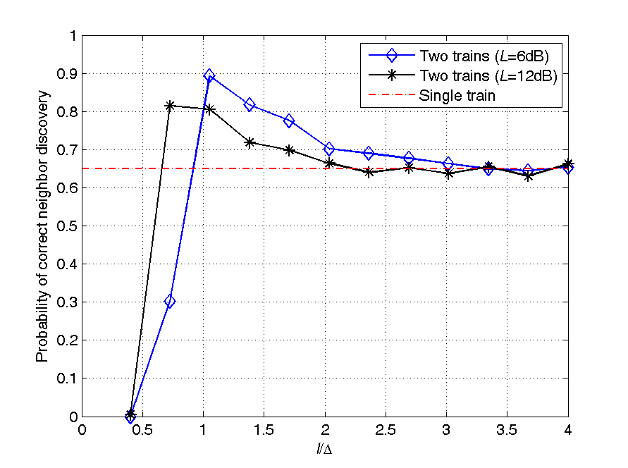
Figure 15: The probability of successful neighbor discovery versus the ratio $l/\Delta$ (see Fig. 8) for the two-train set-up of Fig. 8 with different values of the side lobe attenuation $L$ ($p_{H}=0.15$, $p_{T}=0.15$, $\mathrm{SNR}_{0}=15\,\mathrm{dB}$, $M_{H}=6$ and $\theta=\pi/3$).

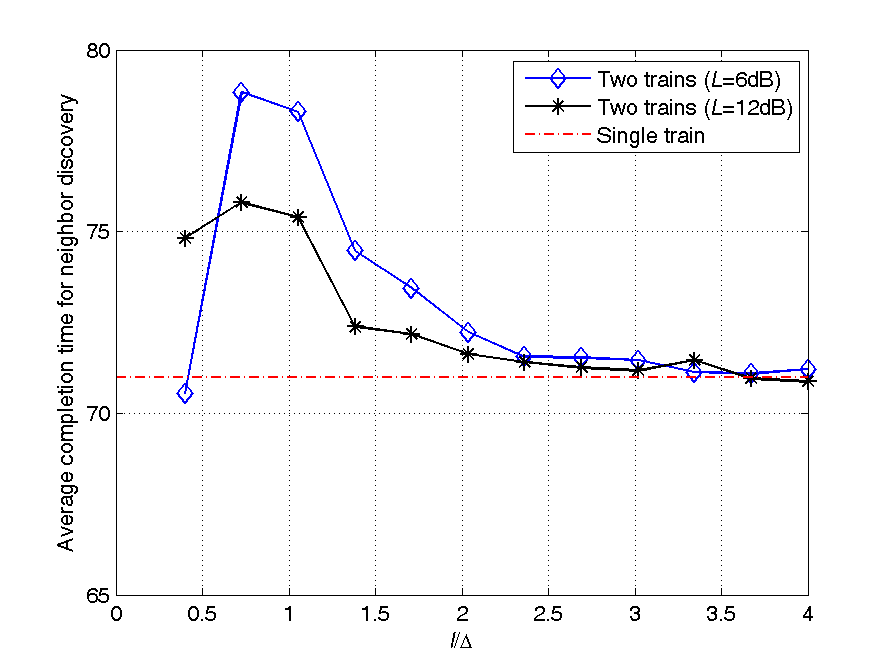
Figure 16: The average time required to complete neighbor discovery versus the ratio $l/\Delta$ (see Fig. 8) for the two-train set-up of Fig. 8 with different values of the side lobe attenuation $L$ ($p_{H}=0.15$, $p_{T}=0.15$, $\mathrm{SNR}_{0}=15\,\mathrm{dB}$, $M_{H}=6$ and $\theta=\pi/3$).

VII Concluding Remarks

Topology discovery in wireless linear networks is a key enabling protocol for application such as wireless train backbone communication. In this work, we have presented a wireless topology discovery protocol (WTDP) that requires minor modification to the current wired topology discovery protocol standard and is able to cope with wireless impairments, such as broadcasting, interference and fading. The proposed WTDP is analyzed under a slotted ALOHA MAC protocol and shows, with the aid of extensive numerical examples, to provide flexible and robust performance under realistic condition including the case of inter-train interference. Interesting future work includes the investigation of the impact of more sophisticated physical layer technologies, such as MIMO, on topology discovery, a more thorough analysis of the effect of fast fading channels, as well as the study of privacy and security issues associated with wireless topology discovery.

References

- [1] A. Kesting, M. Treiber and D. Helbing, “Connectivity statistics of store-and-forward intervehicle communication,” IEEE Trans. Intell. Transp. Syst., vol. 11, no. 1, pp. 172–181, Mar. 2010.
- [2] A. Chakravarthy, K. Song and E. Feron, “Preventing automotive pileup crashes in mixed-communication environments,” IEEE Trans. Intell. Transp. Syst., vol. 10, no. 2, pp. 211–225, Jun. 2009.
- [3] B. van Arem, C. van Driel and R. Visser, “The impact of cooperative adaptive cruise control on traffic-flow characteristics,” IEEE Trans. Intell. Transp. Syst., vol. 7, no. 4, pp. 429–436, Dec. 2006.
- [4] H. Hartenstein, B. Bochow, A. Ebner, M. Lott, M. Radimirsch and D. Vollmer, “Position-aware ad hoc wireless networks for inter-vehicle communications: the Fleetnet project,” in Proc. 2nd ACM international symposium on Mobile ad hoc networking & computing, pp. 259-262, Long Beach, CA, Oct. 2001.
- [5] S. Biswas, R. Tatchikou and F. Dion, “Vehicle-to-vehicle wireless communication protocols for enhancing highway traffic safety,” IEEE Communications Magazine, vol. 44, no. 1, pp. 74-82, Jan. 2006.
- [6] Z. D. Chen, H. T. Kung and D. Vlah, “Ad hoc relay wireless networks over moving vehicles on highways,” in Proc. 2nd ACM international symposium on Mobile ad hoc networking & computing, pp. 247-250, Long Beach, CA, Oct. 2001.
- [7] B. Ning, T. Tang, Z. Y. Gao, F. Yan, F. Y. Wang and D. Zeng, “Intelligent railway system in China,” IEEE Trans. Intell. Transp. Syst., vol. 21, no. 5, pp. 80–83, Sep. 2006.
- [8] IEC 61375-2-5, “Electronic railway equipment-Train communication network-Part 2-5. Ethernet Train Backbone,” Jan. 2012.
- [9] W. Zeng, S. Vasudevan, X. Chen, B. Wang, A. Russell and W. Wei, “Neighbor discovery in wireless networks with multipacket reception,” in Proc. ACM International Symposium on Mobile Ad Hoc Networking and Computing, pp. 3, Paris, France, May 2011.
- [10] Y. Fayyaz, M. Nasim M.Y. Javed, “Maximal weight topology discovery in ad hoc wireless sensor networks,” in proc. IEEE International Conference on Computer and Information Technology, pp. 715-722, Bradford, UK, June 2010.
- [11] M. D. Sarr, F. Delobel, M. Misson and I. Niang, “Automatic discovery of topologies and addressing for linear wireless sensors networks,” in proc. IEEE Wireless Days, pp. 1-7, Dublin, Ireland, Nov. 2012.
- [12] T. Kontos, G.S. Alyfantis, Y. Angelopoulos and S. Hadjiefthymiades, “A topology inference algorithm for wireless sensor networks,” in proc. IEEE Symposium on Computers and Communications, pp. 479-484, Cappadocia, Turkey, July 2012.
- [13] B. Li, W. Feng, L. Zhang and C. Spanos, “DEPEND: density adaptive power efficient neighbor discovery for wearable body sensors,” in proc. IEEE International Conference on Automation Science and Engineering, pp. 581-586, Madison, WI, Aug. 2013.
- [14] M. Nasim, Y. Fayyaz, M.Y. Javed, “Bounded degree energy aware topology discovery in ad hoc wireless sensor networks,” in proc. International Conference on Intelligent Sensors, Sensor Networks and Information Processing, pp.13-18, Melbourne, VIC. Dec. 2009.
- [15] A. Barnawi, R. Hafez, “A time & energy efficient topology discovery and scheduling protocol for wireless sensor networks,” in proc. International Conference on Computational Science and Engineering, vol. 2, no. 1, pp. 570-578, Vancouver, BC, Aug. 2009.
- [16] S. Hermann, “Investigation of IEEE 802.11k-based access point coverage area and neighbor discovery,” in Proc. IEEE Conf. Local Comp. Networks, pp. 949-954, Oct. 2007.
- [17] M. J. McGlynn and S. A. Borbash, “Birthday protocols for low energy deployment and flexible neighbor discovery in ad hoc wireless networks,” in Proc. ACM MobiHoc, pp. 137-145, Long Beach, California, Oct. 2001.
- [18] H. Xie, F. Zeng, P.Wang and Y. Yang, “Research and implementation of fast topology discovery algorithm for Zigbee wireless sensor network,” in Proc. IEEE International Conference on Electronic Measurement & Instruments, vol. 2, no. 1, pp.914-918, Harbin, China, Aug. 2013.
- [19] X. Liu, B. Li, S. Huang and M. Chen, “A ZigBee wireless sensor network topology discovery algorithm,” Computer Engineering, vol. 38, no. 4, Feb. 2012.
- [20] I. Jawhar, X. Li, J. Wu and N. Mohamed, “Backbone discovery in thick wireless linear sensor networks,” in proc. IEEE International Conference on Mobile Ad Hoc and Sensor Systems, pp. 606-611, Philadelphia, PA, Oct. 2014.
- [21] J. Jeon, A. Ephremides, “Neighbor discovery in a wireless sensor network: multipacket reception capability and physical-layer signal processing,”Journal of Communications and Networks, vol. 14, no. 5, Oct. 2012.
- [22] S. A. Borbash, A. Ephremides and M. J. McGlynn, “An asynchronous neighbor discovery algorithm for wireless sensor networks,” Ad Hoc Netw., vol. 5, no. 8, pp. 998–1016, 2007.
- [23] S. Vasudevan, D. Towsley, D. Goeckel and R. Khalili, “Neighbor discovery in wireless networks and the coupon collector’s problem,” in Proc. ACM MobiCom, pp. 181-192, Beijing, China, Sept. 2009.
- [24] S. Vasudevan, J. Kurose, and D. Towsley, “On neighbor discovery in wireless networks with directional antennas,” in Proc. IEEE INFOCOM, vol. 4, pp. 2502-2512, Miami, Florida, Mar. 2005.
- [25] M. Zhang, M. Chan and A.L. Ananda, “Location-aided topology discovery for wireless sensor networks,” in Proc. IEEE International Conference on Communications, pp. 2718-2722, Beijing, China, May 2008.
- [26] H. Wang, F. Richard Yu, L. Zhu, T. Tang, and B. Ning, “A Cognitive Control Approach to Communication-based Train Control (CBTC) Systems,” IEEE Trans. Intelligent Transportation Systems, vol. 16, no. 4, pp. 1676-1689, Aug. 2015.
- [27] L. Zhu, F. Richard Yu, B. Ning, and T. Tang, “Communication-Based Train Control (CBTC) Systems with Cooperative Relaying: Design and Performance Analysis,” IEEE Trans. Veh. Tech., vol. 63, no. 5, pp. 2162-2172, Jun. 2014.
- [28] C. Karlof and D. Wagner, “Secure routing in sensor networks: attacks and countermeasures,” Ad hoc Networks, vol. 1, no. 2, pp. 293–315, 2003.
- [29] M. S. Haghighi, K. Mohamedpour, V. Varadharajan and B. G. Quinn, “Stochastic modeling of hello flooding in slotted CSMA/CA wireless sensor networks,” IEEE Transactions on Information Forensics and Security, vol. 6, no. 4, Dec. 2011.
- [30] Y. C. Hu, A. Perrig, and D. B. Johnson, “Wormhole attacks in wireless networks,” IEEE J. Sel. Areas Commun., vol. 24, no. 2, pp. 370–380, Feb. 2006.
- [31] T. and T. Dimitriou, “LDAC: A localized and decentralized algorithm for efficiently countering wormholes in mobile wireless networks,” Journal of Computer and System Sciences, Vol. 80, no. 3, pp. 618-643, May 2014.
- [32] S. Yoo, S. Kang, and J. Kim, “SERA: a secure energy reliability aware data gathering for sensor networks,” Multimedia Tools Applicat., vo.1, no. 2, pp. 1–30, Jan. 2011.
- [33] K. Saghar, W. Henderson, and D. Kendel, “Formal modelling and analysis of routing protocol security in wireless sensor networks,” in proc. Annual Postgraduate Symposium on the Convergence of Telecommunications, pp. 179–184, Liverpool, June 2009.
- [34] T. M. Cover and J. A. Thomas, Elements of Information Theory, John Wiley & Sons, 2006.
- [35] D. Tse and P. Viswanath, Fundamentals of Wireless Communication, Cambridge University Press, 2005.
- [36] S. Kandukuri and S. Boyd, “Optimal power control in interference-limited fading wireless channels with outage-probability specifications,” IEEE Trans. Wireless Commun., vol. 1, no. 1, pp. 46-55, Jan. 2002.
- [37] D. H. Morris and S. J. Mark, Probability and Statistics, Pearson, 2011.
- [38] J. Janssen and R. Manca, Applied Semi-Markov Processes, Springer, 2006.
- [39] T. S. Rappaport, Wireless Communications: Principles and Practice, Prentice Hall, 2002.