Manipulating quantum wave packets via time-dependent absorption

Abstract

A pulse of matter waves may dramatically change its shape when traversing an absorbing barrier with time-dependent transparency. Here we show that this effect can be utilized for controlled manipulation of spatially-localized quantum states. In particular, in the context of atom-optics experiments, we explicitly demonstrate how the proposed approach can be used to generate spatially shifted, split, squeezed and cooled atomic wave packets. We expect our work to be useful in devising new interference experiments with atoms and molecules and, more generally, to enable new ways of coherent control of matter waves.

I Introduction

The ability to engineer and manipulate the spatial wave function of a quantum particle has far-reaching applications in many areas of physics. One example is the so-called “beam-splitting”, a coherent division of an atomic or molecular wave function into two or more non-overlapping wave packets (WPs), which is indispensable in matter-wave interferometry Cronin et al. (2009); *HGH+12Colloquium; *Arn14DeBroglie. Another example is generation of “squeezed states”, i.e., WPs with a reduced uncertainty in one dynamical variable (at the expense of an increased uncertainty in the conjugate variable) that are widely used to enhance the precision of quantum measurements Giovannetti et al. (2004). To date, various mechanisms of reshaping matter WPs have been explored, some of which utilize time-dependent harmonic traps Castin and Dum (1996), quantum holography Weinacht et al. (1999), spatially homogeneous laser light with time-dependent amplitude in the presence of a spatially inhomogeneous magnetic field Olshanii et al. (2000), periodic potentials Eiermann et al. (2003), time-dependent electric fields in atom chips Nest et al. (2010), finite-length attractive optical lattices with a slowly varying envelope Fabre et al. (2011); *CFV+13Matter, or chaotic scattering dynamics Gattobigio et al. (2012). Here we report an alternative approach based on the principle of time-dependent absorption that has versatile applications.

Figure 1: Illustration of matter pulse carving.

In this paper, we show that a localized quantum WP can be efficiently manipulated – spatially shifted, split, squeezed and cooled – by making it pass through a time-dependent absorbing barrier, i.e., a narrow region of space acting as a particle density sink (see Ref. Muga et al. (2004) for mechanisms and treatment of absorption in quantum systems). The absorbing barrier can be realized in the context of atom-optics with a sheet of laser light intercepting the motion of an atomic cloud (see Fig. 1). The radiation frequency of the laser can be chosen such that a passing atom becomes undetectable due to ionization or a change of its internal state, and thus effectively absorbed. Furthermore, the strength of this absorption process can be made time-dependent by varying the intensity of the laser in accordance with an externally prescribed function of time.

To further exemplify the process of time-dependent absorption, we consider an atom initially (at $t=0$) prepared in a state $\Psi^{(0)}(x)|\mathrm{in}\rangle$, where $|\mathrm{in}\rangle$ denotes an internal state of the atom, and $\Psi^{(0)}(x)$ is a spatially localized WP representing its center-of-mass motion. As the atom traverses a laser light sheet positioned at $x=0$, the laser may trigger an atomic transition from $|\mathrm{in}\rangle$ to another state (or to one of several other states) $|\mathrm{abs}\rangle$ of the atomic spectrum. The probability of the transition is nonzero only inside the light sheet, i.e,. in a close vicinity of the point $x=0$, and can be made to depend on time by externally modifying the intensity of the laser. At some time $t>0$, the atom will be found in a state $\Psi^{(t)}(x)|\mathrm{in}\rangle+\sum\limits_{\mathrm{abs}}\psi_{\mathrm{abs}}^{(t)}(x)|\mathrm{abs}\rangle$, where $\Psi^{(t)}(x)$ and $\psi_{\mathrm{abs}}^{(t)}(x)$ denote spatial wave functions corresponding to the internal states $|\mathrm{in}\rangle$ and $|\mathrm{abs}\rangle$, respectively. In what follows below, we will only be concerned with a projection of the full atomic state on $|\mathrm{in}\rangle$, and will regard the rest of the state, $\sum\limits_{\mathrm{abs}}\psi_{\mathrm{abs}}^{(t)}(x)|\mathrm{abs}\rangle$, as a part that has been removed, or “absorbed”, by the light sheet. It is in this sense that we will be interested in a transformation of the center-of-mass wave function $\Psi$, from $\Psi^{(0)}(x)$ to $\Psi^{(t)}(x)$, induced by the light sheet playing the role of an absorbing barrier.

The problem of a non-relativistic quantum particle interacting with an absorbing barrier has a long history and is a paradigm of the theory of quantum transients Kleber (1994); *CGM09Quantum. The limit of an instantaneously opening or closing barrier, first addressed by Moshinsky, was shown to cause well-pronounced oscillations of the probability density distribution; this effect is known as “diffraction in time” (DIT) and bears close mathematical analogy to optical diffraction of light at an aperture with straight edges Moshinsky (1952); *GK76Possibility; *Mos76Diffraction; *BZ97Diffraction; *MMS99Diffraction; *God02Diffraction; *God03Diffraction; *GM05Generic; *TMB+11Explanation. DIT is generally suppressed if the barrier switching is not sufficiently abrupt del Campo et al. (2007) or if the particle momentum distribution exhibits incoherent thermal broadening Godoy (2009). In a many particle scenario, the interaction between particles is also known to suppress DIT del Campo and Muga (2006).

Here we address the motion of a quantum WP in the presence of an absorbing barrier that may, during some intervals of time, open or close exponentially fast, but yet not fast enough to trigger DIT. We show that this subtle regime, being well within experimental reach, allows for controlled reshaping of the WP through the process of removing (or “carving out”) parts of the probability density profile without a side effect of producing diffraction ripples. Our analysis takes into account finite temperature effects, which are inevitable in any laboratory experiment.

The paper is organized as follows. In Sec. II, we present a general framework for an analytical description of the motion of a quantum particle in the presence of a time-dependent absorbing barrier. In Sec. III, we demonstrate the possibility of controlled manipulation of a spatial wave function of the particle, and, in particular, show how the wave function can be displaced (Sec. III.1), split (Sec. III.2), and squeezed (Sec. III.3). We make concluding remarks in Sec. IV. Technical details are deferred to two Appendixes.

II Theoretical framework

In order to facilitate analytical treatment, we consider a quantum particle of mass $m$ initially represented by a Gaussian WP

$$\Psi^{(0)}(x)=\psi_{\alpha_{0},x_{0},v_{0}}^{(0)}(x)$$

$$\quad\equiv\left(\frac{2\mathrm{Re}(\alpha_{0})}{\pi}\right)^{1/4}e^{-\alpha_{0}(x-x_{0})^{2}+imv_{0}(x-x_{0})/\hbar}\,.$$ (1)

Here, $x_{0}$ and $v_{0}$ represent respectively the mean position and velocity of the particle, and the parameter $\alpha_{0}$ is related to the spatial extent $\sigma$ of the WP through $\sigma^{-2}=2\mathrm{Re}(\alpha_{0})$. Hereinafter however we assume $\alpha_{0}$ to be strictly positive, so that $\alpha_{0}=(2\sigma^{2})^{-1}$. Also, for concreteness, we take $x_{0}<0$, $\sigma\ll|x_{0}|$, and $v_{0}>0$. In other words, the initial WP is assumed to be localized on the semi-infinite interval $x<0$ and moving towards the origin.

After a time $t$ and in the absence of any external forcing, the state $\psi_{\alpha_{0},x_{0},v_{0}}^{(0)}$ would evolve into

$$\psi_{\alpha_{0},x_{0},v_{0}}^{(t)}(x) =\int_{-\infty}^{\infty}dx^{\prime}\,K_{0}^{(t)}(x-x^{\prime})\psi_{\alpha_{0},x_{0},v_{0}}^{(0)}(x^{\prime})$$

$$=e^{i\phi_{t}}\psi_{\alpha_{t},x_{t},v_{0}}^{(0)}(x)\,,$$ (2)

where

$$K_{0}^{(\tau)}(\xi)=\sqrt{\frac{m}{2\pi i\hbar\tau}}\exp\left(i\frac{m\xi^{2}}{2\hbar\tau}\right)$$ (3)

is the free-particle propagator, and the functions $\alpha_{\tau}$, $x_{\tau}$, and $\phi_{\tau}$ are defined as

$$\alpha_{\tau}=\frac{\alpha_{0}}{1+2i\hbar\alpha_{0}\tau/m}\,,$$ (4)

$$x_{\tau}=x_{0}+v_{0}\tau\,,$$ (5)

$$\phi_{\tau}=\frac{mv_{0}^{2}\tau}{2\hbar}-\frac{1}{2}\tan^{-1}\left(\frac{2\hbar\alpha_{0}}{m}\tau\right)\,.$$ (6)

We further imagine that in the course of its motion the particle encounters an infinitesimally thin absorbing barrier positioned at $x=0$. (In a realistic setting, the width of the barrier is assumed to be much smaller than the WP size.) The time-dependent transparency of the barrier is characterized by a real-valued aperture function $\chi_{\tau}$, ranging between 0 (representing zero transparency/complete absorption) and 1 (complete transparency/zero absorption). A propagator, transporting the particle probability amplitude from a source point $x^{\prime}<0$ to a point $x>0$ on the other side of the barrier in time $t>0$, can be written as Goussev (2012, 2013)

$$K^{(t)}(x,x^{\prime})=\int\limits_{0}^{t}d\tau\,\frac{\chi_{\tau}}{2}\left(\frac{x}{t-\tau}-\frac{x^{\prime}}{\tau}\right)K_{0}^{(t-\tau)}(x)K_{0}^{(\tau)}(x^{\prime})\,.$$ (7)

The structure of the propagator $K^{(t)}(x,x^{\prime})$ stems from a superposition of a continuous family of paths, parametrized by time $\tau$. The propagation of the particle along each of these paths consists of three consecutive stages: First, the particle moves freely from the source point $x^{\prime}<0$ to the barrier at the origin in time $\tau$; second, the probability amplitude gets modulated by a factor proportional to the transparency of the barrier $\chi_{\tau}$; third, the particle travels freely to the observation point $x>0$ through the remaining time $(t-\tau)$. The additional factor $\frac{1}{2}\left(\frac{x}{t-\tau}-\frac{x^{\prime}}{\tau}\right)$ has the meaning of the average classical velocity at which the particle crosses the barrier, and is essential for correctly weighing relative contributions of the interfering paths.

In fact, the propagator $K^{(t)}(x,x^{\prime})$, given for $x>0$ by Eq. (7), is an exact solution of the following quantum-mechanical problem (see Ref. Goussev (2013) for full details). In this model $K^{(t)}(x,x^{\prime})$, transporting a wave function from a source point $x^{\prime}<0$ to a point $x\not=0$, is set to satisfy (i) the time-dependent Schrödinger equation

$$\left(i\hbar\frac{\partial}{\partial\tau}+\frac{\hbar^{2}}{2m}\frac{\partial^{2}}{\partial x^{2}}\right)K^{(\tau)}(x,x^{\prime})=0$$ (8)

for $0<\tau<t$ and both $x<0$ and $x>0$, (ii) the initial condition $K^{(0^{+})}(x,x^{\prime})=\delta(x-x^{\prime})$, (iii) Dirichlet boundary conditions at $x=\pm\infty$ for negative imaginary times, i.e, $K^{(-i|\tau|)}(\pm\infty,x^{\prime})=0$, and (iv) two matching conditions relating the propagator and its spatial derivative at $x<0$ to those at $x>0$, namely

$$K^{(\tau)}(x,x^{\prime})\big{|}_{x=0^{-}}^{x=0^{+}} =-(1-\chi_{\tau})K_{0}^{(\tau)}(x-x^{\prime})\big{|}_{x=0}\,,$$ (9)

$$\frac{\partial K^{(\tau)}(x,x^{\prime})}{\partial x}\bigg{|}_{x=0^{-}}^{x=0^{+}} =-(1-\chi_{\tau})\frac{\partial K_{0}^{(\tau)}(x-x^{\prime})}{\partial x}\bigg{|}_{x=0}\,,$$ (10)

for $0<\tau<t$. Here, $K_{0}$ denotes the free-particle propagator defined by Eq. (3). The matching conditions (9) and (10) are a time-dependent quantum-mechanical version of the absorbing (“black-screen”) boundary conditions proposed by Kottler in the context of stationary wave optics Kottler (1923); *Kot65Diffraction; in their original time-independent formulation, Kottler boundary conditions can be viewed as a mathematical justification of Kirchhoff diffraction theory.

The wave function transmitted through the barrier at time $t$ is given by

$$\Psi^{(t)}(x)=\Psi_{\alpha_{0},x_{0},v_{0}}^{(t)}(x)\equiv\int\limits_{-\infty}^{\infty}dx^{\prime}\,K^{(t)}(x,x^{\prime})\psi_{\alpha_{0},x_{0},v_{0}}^{(0)}(x^{\prime})$$

$$\;=\int\limits_{0}^{t}d\tau\,\frac{\chi_{\tau}}{2}\left(\frac{x}{t-\tau}+\frac{\alpha_{\tau}v_{0}}{\alpha_{t_{0}}}\right)K_{0}^{(t-\tau)}(x)\psi_{\alpha_{0},x_{0},v_{0}}^{(\tau)}(0)\,,$$ (11)

where $t_{0}=|x_{0}|/v_{0}$ represents the time needed for the corresponding classical particle to reach the barrier. Here however we choose to focus on a phase-space representation of the wave function as provided by the Husimi distribution [See; e.g.; ][]Bal14Quantum

$$H_{\alpha_{0},x_{0},v_{0}}^{(t)}(\tilde{x},\tilde{v})=\left|\langle\psi_{\alpha_{0},\tilde{x},\tilde{v}}^{(0)}|\Psi_{\alpha_{0},x_{0},v_{0}}^{(t)}\rangle\right|^{2}\,.$$ (12)

The Husimi distribution quantifies the overlap between the time-evolved state $\Psi_{\alpha_{0},x_{0},v_{0}}^{(t)}$ and a probe Gaussian WP centered in phase space around $(\tilde{x},\tilde{v})$ and characterized by the spatial dispersion $\sigma=1/\sqrt{2\alpha_{0}}$. Hereinafter, we assume $0<\sigma\ll\tilde{x}$; this implies that we only examine the wave function $\Psi_{\alpha_{0},x_{0},v_{0}}^{(t)}(x)$ deep inside the transmission region. Then, using Eq. (11) we obtain

$$\langle\psi_{\alpha_{0},\tilde{x},\tilde{v}}^{(0)}| \Psi_{\alpha_{0},x_{0},v_{0}}^{(t)}\rangle=\int\limits_{0}^{t}d\tau\,\frac{\chi_{\tau}}{2}\left(\frac{\alpha_{t-\tau}\tilde{v}}{\alpha_{\tilde{t}}}+\frac{\alpha_{\tau}v_{0}}{\alpha_{t_{0}}}\right)$$

$$\qquad\times\left[\psi_{\alpha_{0},\tilde{x},\tilde{v}}^{(\tau-t)}(0)\right]^{*}\,\psi_{\alpha_{0},x_{0},v_{0}}^{(\tau)}(0)\,,$$ (13)

where $\tilde{t}=\tilde{x}/\tilde{v}$ and the asterisk represents complex conjugation. The integrand in Eq. (13), unlike that in Eq. (11), is free of singular points on the closed interval $0\leq\tau\leq t$. This fact makes formula (13) an efficient tool for analytical and numerical inspection of the part of the WP transmitted through the absorbing barrier.

Non-zero temperature, ubiquitous in any laboratory experiment, manifests itself as an incoherent broadening of the initial velocity distribution of the particle. In order to account for this broadening, we describe the particle state in terms of a time-dependent density matrix

$$\rho_{\alpha_{0},x_{0},v_{0},\Delta v}^{(\tau)}$$

$$\quad=\frac{1}{\sqrt{\pi}}\int_{-\infty}^{\infty}\frac{dv}{\Delta v}\,e^{-(v-v_{0})^{2}/\Delta v^{2}}|\Psi_{\alpha_{0},x_{0},v}^{(\tau)}\rangle\langle\Psi_{\alpha_{0},x_{0},v}^{(\tau)}|\,,$$ (14)

where $\Delta v$ quantifies the width of the thermal spread of the initial velocity. The corresponding finite-temperature Husimi distribution reads

$$\mathcal{H}_{\alpha_{0},x_{0},v_{0},\Delta v}^{(t)}(\tilde{x},\tilde{v})=\mathrm{tr}\left(\rho_{\alpha_{0},x_{0},v_{0},\Delta v}^{(t)}|\psi_{\alpha_{0},\tilde{x},\tilde{v}}^{(0)}\rangle\langle\psi_{\alpha_{0},\tilde{x},\tilde{v}}^{(0)}|\right)$$

$$\qquad=\frac{1}{\sqrt{\pi}}\int\limits_{-\infty}^{\infty}\frac{dv}{\Delta v}\,e^{-(v-v_{0})^{2}/\Delta v^{2}}H_{\alpha_{0},x_{0},v}^{(t)}(\tilde{x},\tilde{v})\,,$$ (15)

where tr denotes the trace. Substituting Eqs. (12) and (13) into Eq. (15), we obtain

$$\mathcal{H}_{\alpha_{0},x_{0},v_{0},\Delta v}^{(t)}(\tilde{x},\tilde{v})=\frac{1}{4}\int\limits_{0}^{t}d\tau\int\limits_{0}^{t}d\tau^{\prime}\,\chi_{\tau}\chi_{\tau^{\prime}}\left[\psi_{\alpha_{0},\tilde{x},\tilde{v}}^{(\tau-t)}(0)\right]^{*}\psi_{\alpha_{0},\tilde{x},\tilde{v}}^{(\tau^{\prime}-t)}(0)\;\Phi_{\alpha_{0},\tilde{x},\tilde{v},x_{0},v_{0},\Delta v}^{(t,\tau,\tau^{\prime})}\,,$$ (16)

where

$$\Phi_{\alpha_{0},\tilde{x},\tilde{v},x_{0},v_{0},\Delta v}^{(t,\tau,\tau^{\prime})}=\frac{1}{\sqrt{\pi}}\int\limits_{-\infty}^{\infty}\frac{dv}{\Delta v}\,e^{-(v-v_{0})^{2}/\Delta v^{2}}\left(\frac{\alpha_{t-\tau}\tilde{v}}{\alpha_{\tilde{t}}}+\frac{\alpha_{\tau}v}{\alpha_{|x_{0}|/v}}\right)\left(\frac{\alpha_{t-\tau^{\prime}}\tilde{v}}{\alpha_{\tilde{t}}}+\frac{\alpha_{\tau^{\prime}}v}{\alpha_{|x_{0}|/v}}\right)^{\!*}\psi_{\alpha_{0},x_{0},v}^{(\tau)}(0)\left[\psi_{\alpha_{0},x_{0},v}^{(\tau^{\prime})}(0)\right]^{*}.$$ (17)

In view of the identity $\frac{v}{\alpha_{|x_{0}|/v}}=\frac{v}{\alpha_{0}}+\frac{2i\hbar|x_{0}|}{m}$, the integral in Eq. (17) is Gaussian in nature and can be evaluated analytically. (See Appendix A for the calculation and exact expression.)

Below we use the Husimi distributions given by Eqs. (12) and (13) and Eqs. (16) and (17) to analyze several scenarios of WP engineering corresponding to specific forms of the aperture function $\chi_{\tau}$.

III Wave packet engineering

III.1 Spatial shifting

We first investigate physical effects produced by an exponentially opening (closing) barrier. Thus, we consider

$$\chi_{\tau}=\chi_{0}\,e^{\gamma\tau}\,,$$ (18)

where $\gamma$ is the rate of change of the barrier transparency and $\chi_{0}$ is its initial value. While an explicit evaluation of the corresponding Husimi distribution is not feasible, a significant analytical insight can be gained in an asymptotic regime, defined by

$$1\ll\frac{|x_{0}|}{\sigma}\lesssim\frac{v_{0}t}{2\sigma}\ll\frac{\sigma}{2\lambdabar}\,,$$ (19)

where $\lambdabar=\hbar/(mv_{0})$ is the reduced de Broglie wavelength of the particle. The first of the three conditions combined in Eq. (19), $\sigma\ll|x_{0}|$, has already been used in deriving Eq. (11). The second inequality, $2|x_{0}|\lesssim v_{0}t$, is needed to ensure that, at time $t$, the particle has “passed” the barrier and the dominant part of the WP is well localized in the transmission region; under this condition, the Husimi distribution of the transmitted WP is accurately represented by Eqs. (12) and (13). Finally, the third inequality, $\lambdabar\ll\sigma^{2}/(v_{0}t)$, expresses the semiclassical limit, in which time variations of the spatial width of the WP can be effectively neglected; this limit is commonly known as a “frozen Gaussian” regime Heller (1981).

Adopting the semiclassical regime specified by Eq. (19) and further assuming that

$$|\gamma|\ll\frac{2|x_{0}|v_{0}}{\sigma^{2}}\,,$$ (20)

we use the method of steepest descent to evaluate the pure-state Husimi distribution $H_{\alpha_{0},x_{0},v_{0}}^{(t)}(\tilde{x},\tilde{v})$ analytically. (See Appendix B for details of the calculation.) In particular, we show that $H_{\alpha_{0},x_{0},v_{0}}^{(t)}(\tilde{x},\tilde{v})$ is peaked at the phase-space point $(\tilde{x},\tilde{v})=(x_{t}+\Delta x,v_{0})$ with

$$\Delta x=-\frac{\gamma\sigma^{2}}{v_{0}}\,.$$ (21)

This means that the transmitted WP appears to be spatially shifted compared to the counterpart free-particle WP centered at $(x_{t},v_{0})$. The shift is proportional to the rate of change of the barrier transparency and can be positive (advanced WP) as well as negative (delayed WP). The average velocity of the particle however remains unaffected by the barrier. The analysis also reveals that the overall transmission probability is given approximately by $\chi_{t_{0}}^{2}$.

In order to further explore the effect of the WP shift, we compute the pure-state and finite-temperature Husimi distributions by numerically evaluating the integrals in Eqs. (13) and (16) respectively. To this end, we consider a cloud of ultra-cold atoms characterized by $m=86.909$ u (the mass of a ⁸⁷Rb atom), $\sigma=30$ $\mu$m, $v_{0}=3$ mm/s, and $\Delta v=0.1$ mm/s. (A cloud of magnetically levitated ⁸⁷Rb atoms with similar parameters has been recently used by Jendrzejewski et al. to experimentally demonstrate coherent backscattering of ultra-cold atoms in a disordered potential Jendrzejewski et al. (2012).) The cloud is initially centered at $x_{0}=-0.15$ mm and the propagation time is set to be $t=100$ ms, implying that $x_{t}=0.15$ mm $=|x_{0}|$ and $t_{0}=50$ ms $=t/2$. (In the experiment in Ref. Jendrzejewski et al. (2012), it was possible to let the atomic cloud evolve for as long as 150 ms before performing imaging.) Since for the chosen set of parameters $\lambdabar\simeq 244$ nm, the system is in the semiclassical regime specified by Eq. (19). Furthermore, the value of $|\gamma|$ in all computations below is taken not to exceed 225 s^-1, which ensures that the restriction given by Eq. (20) is fulfilled.

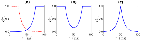
Figure 2: Aperture function given by (a) Eq. (22) with $\gamma=100$ s^-1 (solid blue curve) and $\gamma=-100$ s^-1 (dashed red curve), (b) Eq. (23) with $\gamma=100$ s^-1, and (c) Eq. (24) with $\gamma=100$ s^-1.

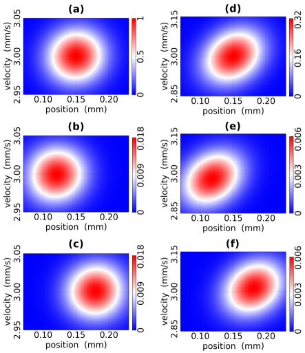
Figure 3: Husimi distributions for a ⁸⁷Rb atom in a pure (a-c) and a mixed, finite-temperature (d-f) state, i.e., $H_{\alpha_{0},x_{0},v_{0}}^{(t)}(\tilde{x},\tilde{v})$ and $\mathcal{H}_{\alpha_{0},x_{0},v_{0},\Delta v}^{(t)}(\tilde{x},\tilde{v})$ respectively. System parameters are: $m=86.909$ u, $\sigma=30$ $\mu$m, $x_{0}=-0.15$ mm, $v_{0}=3$ mm/s, $\Delta v=0.1$ mm/s, and $t=100$ ms. The aperture function is defined by Eq. (22). $\gamma=0$ in (a) and (d), $\gamma=100$ s^-1 in (b) and (e), and $\gamma=-100$ s^-1 in (c) and (f).

In the semiclassical regime, the shape of the transmitted WP depends predominantly on the form of the aperture function $\chi_{\tau}$ in the vicinity of the time $t_{0}$, at which the classical particle crosses the barrier, and is largely insensitive to the behavior of $\chi_{\tau}$ close to the ends of the time interval $0\leq\tau\leq t$. So, in order to increase the overall transmission probability we consider the aperture function (see Fig. 2(a))

$$\chi_{\tau}=\min\left\{e^{\gamma(\tau-t_{1})}\,,\;1\right\}\,,\quad t_{1}=\left\{\begin{array}[]{cl}\frac{3t_{0}}{2}&\mathrm{if}\;\gamma>0\\[5.69046pt] \frac{t_{0}}{2}&\mathrm{if}\;\gamma\leq 0\end{array}\right.$$ (22)

when numerically evaluating the integrals in Eqs. (13) and (16), instead of the one given by Eq. (18). Figure 3 shows the corresponding Husimi distributions $H_{\alpha_{0},x_{0},v_{0}}^{(t)}(\tilde{x},\tilde{v})$ and $\mathcal{H}_{\alpha_{0},x_{0},v_{0},\Delta v}^{(t)}(\tilde{x},\tilde{v})$ as functions of position $\tilde{x}$ and velocity $\tilde{v}$ for different values of $\gamma$. Figure 3(a-c) represent the pure state case, and Fig. 3(d-f) correspond to the case of a mixed, finite-temperature state. The spatial shift of the Husimi distribution is well pronounced in the figure, and its numerical value is found to be in good agreement with the predictions of Eq. (21), i.e., $\Delta x=\mp 30$ $\mu$m for $\gamma=\pm 100$ s^-1. It is interesting to observe a slight change of the average velocity of the particle in the mixed state case (see Fig. 3(e,f)). This velocity shift stems from the fact that WPs with different average velocities, comprising the mixed state, arrive at the barrier at different times and, as a result, are subject to different values of the transparency function. As we show later, this effect can be exploited to reduce the phase-space uncertainty of (and effectively cool down) an atomic cloud.

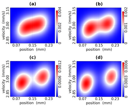
Figure 4: Husimi distribution $\mathcal{H}_{\alpha_{0},x_{0},v_{0},\Delta v}^{(t)}(\tilde{x},\tilde{v})$ for a mixed state, characterized by the same set of parameters as in Fig. 3(d-f), in the presence of an absorbing barrier specified by Eq. (23) with (a) $\gamma=125$ s^-1, (b) $\gamma=150$ s^-1, (c) $\gamma=175$ s^-1, and (d) $\gamma=225$ s^-1.

III.2 Splitting

We now consider a different scenario in which the aperture function $\chi_{\tau}$ in the vicinity of $t_{0}$ is given by an equally weighted sum of an increasing and a decaying exponential, $e^{\gamma\tau}$ and $e^{-\gamma\tau}$. As before, in order to increase the overall transmission probability, we take $\chi_{\tau}$ to be unity around the ends of the interval $0\leq\tau\leq t$. Thus, we choose (see Fig. 2(b))

$$\chi_{\tau}=\min\left\{\frac{\cosh[\gamma(\tau-t_{0})]}{\cosh(\gamma t_{0}/2)}\,,\;1\right\}\,.$$ (23)

Figure 4 shows the response of a finite-temperature WP, characterized by the same set of parameters as above, to an absorbing barrier specified by Eq. (23). As the rate $\gamma$ increases, the WP stretches and eventually splits in two practically non-overlapping parts. A slight difference between the average velocities of the two parts has the same physical origin as in the shifting scenario (see Fig. 3(e,f)).

The absorption-based WP splitting mechanism presented here may be utilized in designing new types of matter-wave interferometers. Indeed, the two WPs produced by the splitting continue propagating along the same path in the coordinate space. If this path traverses a region with an external potential that is nonuniform in space and time, such as a time-dependent disorder, then the two WPs will accumulate different phases in the course of their motion, and their subsequent recombination will give rise to an interference pattern. The interference pattern can subsequently be used to extract information about the potential.

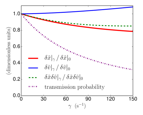
Figure 5: Relative spatial (solid red curve), velocity (solid blue curve) and phase-space (dashed green curve) uncertainties, and total transmission probability (dashed-dotted purple curve) as functions of the rate $\gamma$ for the aperture function defined in Eq. (24). All system parameters are the same as in Fig. 3(d-f) and Fig. 4.

III.3 Squeezing and cooling

Finally, we consider a scenario in which the barrier first opens exponentially until the time $t_{0}$ and then closes exponentially, so that the aperture function reads (see Fig. 2(c))

$$\chi_{\tau}=e^{-\gamma|\tau-t_{0}|}\,,\quad\gamma>0\,.$$ (24)

In this case, the Husimi distribution $\mathcal{H}_{\alpha_{0},x_{0},v_{0},\Delta v}^{(t)}(\tilde{x},\tilde{v})$ of a transmitted WP for $\gamma>0$ appears to be squeezed in the $\tilde{x}$ direction and stretched in the $\tilde{v}$ direction compared to the free-particle case. Figure 5 shows the $\gamma$-dependence of position (solid red curve) and velocity (solid blue curve) dispersions of the WP, $\delta\tilde{x}$ and $\delta\tilde{v}$ respectively, computed with respect to the Husimi distribution:

$$\delta(\cdot)=\left[\int d\tilde{x}d\tilde{v}(\cdot)^{2}\mathcal{H}-\left(\int d\tilde{x}d\tilde{v}(\cdot)\mathcal{H}\right)^{2}\right]^{1/2}\,.$$ (25)

The initial WP is characterized by the same set of parameters as above.

It is interesting to observe that as $\gamma$ grows the decrease of $\delta\tilde{x}$ occurs at a higher rate than the increase of $\delta\tilde{v}$. For instance, at $\gamma=150$ s^-1 the spatial dispersion is reduced by over 20% compared to its value in the absence of a barrier, whereas the corresponding relative increase in the velocity dispersion is less than 10%. This means that the overall phase-space uncertainty $\delta\tilde{x}(m\delta\tilde{v})$ decreases with growing $\gamma$. The $\gamma$-dependence of the relative phase-space uncertainty is shown by a dashed green curve in Fig. 5. For the given set of parameters, $\delta\tilde{x}(m\delta\tilde{v})\big{|}_{\gamma=0}\simeq 3.12\hbar$, whereas $\delta\tilde{x}(m\delta\tilde{v})\big{|}_{\gamma=150\,\mathrm{s}^{-1}}\simeq 2.66\hbar$. (We note that the Heisenberg uncertainty principle, with all averages computed with respect to a Husimi distribution function, states that $\delta\tilde{x}(m\delta\tilde{v})\geq\hbar$ Ballentine (2014).) In other words, the velocity spread of the WP at a finite $\gamma$ is closer to the Heisenberg limit $\delta\tilde{v}_{H}=\hbar/\delta\tilde{x}$ than that of the corresponding free-particle WP. This in turn means that the moving particle gets effectively cooled down by the absorbing barrier. The cooling occurs through absorption of those components of the mixed state that have the largest deviations of the velocity from its average value. (The dotted-dashed purple curve in Fig. 5 shows the decay of the overall transmission probability defined as $\int_{0}^{+\infty}d\tilde{x}\int_{-\infty}^{+\infty}d\tilde{v}\,\mathcal{H}$.) In a sense, the effect is similar in nature to that of evaporative cooling Anderson et al. (1995).

IV Conclusion

In summary, we have demonstrated that a moving WP of quantum matter can be flexibly manipulated with the help of a thin stationary absorbing barrier whose transparency changes in time according to an externally prescribed protocol. In particular, the WP transmitted through the barrier may be spatially shifted, split in two, or squeezed and cooled compared to the corresponding WP in free space. The reported effects can be observed in a laboratory setting using a cloud of ultra-cold atoms akin to that produced in experiments in Ref. Jendrzejewski et al. (2012) and a laser light sheet of variable intensity.

In this paper, being mainly interested in a proof-of-principle demonstration of absorption-based WP control, we have only considered barrier apertures of relatively simple, compact functional forms. In real world situations however aperture function optimization could be used to steer the wave function into a desired target state. (See Ref. Nest et al. (2010) for an example of the optimization approach in the context of control of atomic WPs in atom chips.) Other important extensions of the present work would be to generalize our theory to the case of interacting particles and to investigate if there are any new effects produced by a time-dependent absorbing barrier of a finite spatial extent.

We believe that our findings may become of considerable value in areas of physics concerned with matter-wave interferometry, quantum control, and quantum metrology, as well as facilitate better understanding of effects of absorption in quantum systems.

Appendix A Evaluation of $\Phi_{\alpha_{0},\tilde{x},\tilde{v},x_{0},v_{0},\Delta v}^{(t,\tau,\tau^{\prime})}$

Here we derive a closed form expression for the function $\Phi_{\alpha_{0},\tilde{x},\tilde{v},x_{0},v_{0},\Delta v}^{(t,\tau,\tau^{\prime})}$ defined by Eq. (17).

Using Eq. (2), we write

$$\psi_{\alpha_{0},x_{0},v}^{(\tau)}(0) =\left(\frac{2\alpha_{\tau}^{2}}{\pi\alpha_{0}}\right)^{1/4}\exp\left(-\alpha_{\tau}(x_{0}+v\tau)^{2}-i\frac{mv}{\hbar}(x_{0}+v\tau)+i\frac{mv^{2}\tau}{2\hbar}\right)$$

$$=\left(\frac{2\alpha_{\tau}^{2}}{\pi\alpha_{0}}\right)^{1/4}\exp\left[-\left(\alpha_{\tau}\tau+i\frac{m}{2\hbar}\right)\tau v^{2}-2\left(\alpha_{\tau}\tau+i\frac{m}{2\hbar}\right)x_{0}v-\alpha_{\tau}x_{0}^{2}\right]$$

$$=\left(\frac{2\alpha_{\tau}^{2}}{\pi\alpha_{0}}\right)^{1/4}\exp\left(-i\frac{m\tau\alpha_{\tau}}{2\hbar\alpha_{0}}v^{2}-i\frac{mx_{0}\alpha_{\tau}}{\hbar\alpha_{0}}v-\alpha_{\tau}x_{0}^{2}\right)\,.$$

In the last line we have used the identity $\alpha_{\tau}\tau+\frac{im}{2\hbar}=i\frac{m\alpha_{\tau}}{2\hbar\alpha_{0}}$. Similarly, we have

$$\left[\psi_{\alpha_{0},x_{0},v}^{(\tau^{\prime})}(0)\right]^{*}= \left(\frac{2(\alpha_{\tau^{\prime}}^{*})^{2}}{\pi\alpha_{0}}\right)^{1/4}$$

$$\times\exp\left(i\frac{m\tau^{\prime}\alpha_{\tau^{\prime}}^{*}}{2\hbar\alpha_{0}}v^{2}+i\frac{mx_{0}\alpha_{\tau^{\prime}}^{*}}{\hbar\alpha_{0}}v-\alpha_{\tau^{\prime}}^{*}x_{0}^{2}\right)\,.$$

Therefore

$$e^{-(v-v_{0})^{2}/\Delta v^{2}} \psi_{\alpha_{0},x_{0},v}^{(\tau)}(0)\left[\psi_{\alpha_{0},x_{0},v}^{(\tau^{\prime})}(0)\right]^{*}$$

$$=\sqrt{\frac{2R\alpha_{0}}{\pi}}\exp\left(-Av^{2}+Bv-C\right)\,,$$

where

$$A =\frac{1}{\Delta v^{2}}+i\frac{m\left(\tau\alpha_{\tau}-\tau^{\prime}\alpha_{\tau^{\prime}}^{*}\right)}{2\hbar\alpha_{0}}\,,$$

$$B =\frac{2v_{0}}{\Delta v^{2}}-i\frac{mx_{0}\left(\alpha_{\tau}-\alpha_{\tau^{\prime}}^{*}\right)}{\hbar\alpha_{0}}\,,$$

$$C =\frac{v_{0}^{2}}{\Delta v^{2}}+\left(\alpha_{\tau}+\alpha_{\tau^{\prime}}^{*}\right)x_{0}^{2}\,,$$

$$R =\frac{\alpha_{\tau}\alpha_{\tau^{\prime}}^{*}}{\alpha_{0}^{2}}\,.$$

Also, using $\frac{v}{\alpha_{|x_{0}|/v}}=\frac{v}{\alpha_{0}}+i\frac{2\hbar|x_{0}|}{m}=\frac{v}{\alpha_{0}}-i\frac{2\hbar x_{0}}{m}$, we write

$$\left(\frac{\alpha_{t-\tau}\tilde{v}}{\alpha_{\tilde{t}}}+\frac{\alpha_{\tau}v}{\alpha_{|x_{0}|/v}}\right)\left(\frac{\alpha_{t-\tau^{\prime}}\tilde{v}}{\alpha_{\tilde{t}}}+\frac{\alpha_{\tau^{\prime}}v}{\alpha_{|x_{0}|/v}}\right)^{\!*} =\left(\frac{\alpha_{t-\tau}\tilde{v}}{\alpha_{\tilde{t}}}-i\frac{2\hbar x_{0}\alpha_{\tau}}{m}+\frac{\alpha_{\tau}}{\alpha_{0}}v\right)\left(\frac{\alpha_{t-\tau^{\prime}}^{*}\tilde{v}}{\alpha_{\tilde{t}}^{*}}+i\frac{2\hbar x_{0}\alpha_{\tau^{\prime}}^{*}}{m}+\frac{\alpha_{\tau^{\prime}}^{*}}{\alpha_{0}}v\right)$$

$$=Rv^{2}+Sv+T\,,$$

where

$$S =\frac{\tilde{v}}{\alpha_{0}}\left(\frac{\alpha_{\tau}\alpha_{t-\tau^{\prime}}^{*}}{\alpha_{\tilde{t}}^{*}}+\frac{\alpha_{t-\tau}\alpha_{\tau^{\prime}}^{*}}{\alpha_{\tilde{t}}}\right)\,,$$

$$T =\left(\frac{\alpha_{t-\tau}\tilde{v}}{\alpha_{\tilde{t}}}-i\frac{2\hbar x_{0}\alpha_{\tau}}{m}\right)\left(\frac{\alpha_{t-\tau^{\prime}}^{*}\tilde{v}}{\alpha_{\tilde{t}}^{*}}+i\frac{2\hbar x_{0}\alpha_{\tau^{\prime}}^{*}}{m}\right)\,.$$

Substituting the above expressions into Eq. (17), we obtain

$$\Phi_{\alpha_{0},\tilde{x},\tilde{v},x_{0},v_{0},\Delta v}^{(t,\tau,\tau^{\prime})} =\frac{\sqrt{2R\alpha_{0}}}{\pi\Delta v}\int\limits_{-\infty}^{+\infty}\,dv\left(Rv^{2}+Sv+T\right)\exp\left(-Av^{2}+Bv-C\right)$$

$$=\frac{1}{\Delta v}\sqrt{\frac{2R\alpha_{0}}{\pi}}\left(\frac{T}{A^{1/2}}+\frac{BS+R}{2A^{3/2}}+\frac{B^{2}R}{4A^{5/2}}\right)\exp\left(\frac{B^{2}}{4A}-C\right)\,.$$

The last expression can be directly adopted for numerical evaluation of the thermal-state Husimi distribution.

Finally, we note that, as expected, the last expression respects the identity

$$\lim_{\Delta v\rightarrow 0} \Phi_{\alpha_{0},\tilde{x},\tilde{v},x_{0},v_{0},\Delta v}^{(t,\tau,\tau^{\prime})}$$

$$\quad=\left(\frac{\alpha_{t-\tau}\tilde{v}}{\alpha_{\tilde{t}}}+\frac{\alpha_{\tau}v_{0}}{\alpha_{t_{0}}}\right)\left(\frac{\alpha_{t-\tau^{\prime}}\tilde{v}}{\alpha_{\tilde{t}}}+\frac{\alpha_{\tau^{\prime}}v_{0}}{\alpha_{t_{0}}}\right)^{\!*}$$

$$\quad\quad\times\psi_{\alpha_{0},x_{0},v_{0}}^{(\tau)}(0)\left[\psi_{\alpha_{0},x_{0},v_{0}}^{(\tau^{\prime})}(0)\right]^{*}$$

with $t_{0}=|x_{0}|/v_{0}$, thus recovering

$$\lim_{\Delta v\rightarrow 0}\mathcal{H}_{\alpha_{0},x_{0},v_{0},\Delta v}^{(t)}(\tilde{x},\tilde{v})=H_{\alpha_{0},x_{0},v_{0}}^{(t)}(\tilde{x},\tilde{v})\,.$$

Appendix B Peak of $H_{\alpha_{0},x_{0},v_{0}}^{(t)}(\tilde{x},\tilde{v})$ for $\chi_{\tau}=\chi_{0}e^{\gamma\tau}$ in the semiclassical regime

Here we provide a derivation of Eq. (21).

In the semiclassical regime, $1\ll\frac{|x_{0}|}{\sigma}\lesssim\frac{v_{0}t}{2\sigma}\ll\frac{\sigma}{2\lambdabar}$ with $\lambdabar=\hbar/(mv_{0})$, we define a small parameter

$$\epsilon=\frac{\hbar t}{m\sigma^{2}}\ll 1\,.$$

($\epsilon$ plays the role of an effective Planck’s constant.) Using $\alpha_{\tau}=\alpha_{0}\left(1+i\frac{\tau}{t}\epsilon\right)^{-1}=\alpha_{0}+\mathcal{O}(\epsilon)$ for $0<\tau<t$, we write

$$\psi_{\alpha_{0},x_{0},v_{0}}^{(\tau)}(0) =\left(\frac{2\alpha_{\tau}^{2}}{\pi\alpha_{0}}\right)^{1/4}\exp\left(-\alpha_{\tau}(x_{0}+v_{0}\tau)^{2}-i\frac{mv_{0}}{\hbar}(x_{0}+v_{0}\tau)+i\frac{mv_{0}^{2}\tau}{2\hbar}\right)$$

$$=\left[\left(\frac{2\alpha_{0}}{\pi}\right)^{1/4}+\mathcal{O}(\epsilon)\right]\exp\left(-\alpha_{0}(x_{0}+v_{0}\tau)^{2}-i\frac{mv_{0}}{\hbar}(x_{0}+v_{0}\tau)+i\frac{mv_{0}^{2}\tau}{2\hbar}+\mathcal{O}(\epsilon)\right)$$

$$\simeq\left(\frac{2\alpha_{0}}{\pi}\right)^{1/4}\exp\left[-\alpha_{0}v_{0}^{2}\tau^{2}-\left(2\alpha_{0}x_{0}v_{0}+i\frac{mv_{0}^{2}}{2\hbar}\right)\tau-\alpha_{0}x_{0}^{2}-i\frac{mx_{0}v_{0}}{\hbar}\right]\,.$$

Similarly,

$$\left[\psi_{\alpha_{0},x_{0},v_{0}}^{(\tau^{\prime})}(0)\right]^{*}\simeq\left(\frac{2\alpha_{0}}{\pi}\right)^{1/4}\exp\left[-\alpha_{0}v_{0}^{2}\tau^{\prime 2}-\left(2\alpha_{0}x_{0}v_{0}-i\frac{mv_{0}^{2}}{2\hbar}\right)\tau^{\prime}-\alpha_{0}x_{0}^{2}+i\frac{mx_{0}v_{0}}{\hbar}\right]\,,$$

$$\left[\psi_{\alpha_{0},\tilde{x},\tilde{v}}^{(\tau-t)}(0)\right]^{*}\simeq\left(\frac{2\alpha_{0}}{\pi}\right)^{1/4}\exp\left[-\alpha_{0}\tilde{v}^{2}(\tau-t)^{2}-\left(2\alpha_{0}\tilde{x}\tilde{v}-i\frac{m\tilde{v}^{2}}{2\hbar}\right)(\tau-t)-\alpha_{0}\tilde{x}^{2}+i\frac{m\tilde{x}\tilde{v}}{\hbar}\right]\,,$$

$$\psi_{\alpha_{0},\tilde{x},\tilde{v}}^{(\tau^{\prime}-t)}(0)\simeq\left(\frac{2\alpha_{0}}{\pi}\right)^{1/4}\exp\left[-\alpha_{0}\tilde{v}^{2}(\tau^{\prime}-t)^{2}-\left(2\alpha_{0}\tilde{x}\tilde{v}+i\frac{m\tilde{v}^{2}}{2\hbar}\right)(\tau^{\prime}-t)-\alpha_{0}\tilde{x}^{2}-i\frac{m\tilde{x}\tilde{v}}{\hbar}\right]\,.$$

Then,

$$\left[\psi_{\alpha_{0},\tilde{x},\tilde{v}}^{(\tau-t)}(0)\right]^{*}\psi_{\alpha_{0},\tilde{x},\tilde{v}}^{(\tau^{\prime}-t)}(0)\,\psi_{\alpha_{0},x_{0},v_{0}}^{(\tau)}(0)\left[\psi_{\alpha_{0},x_{0},v_{0}}^{(\tau^{\prime})}(0)\right]^{*}$$

$$\qquad\simeq\frac{2\alpha_{0}}{\pi}\exp\big{[}-U\left(\tau^{2}+\tau^{\prime 2}\right)-\left(V_{R}-iV_{I}\right)\tau$$

$$\qquad\qquad\qquad\qquad-\left(V_{R}+iV_{I}\right)\tau^{\prime}-W\big{]}\,,$$

where

$$U=\alpha_{0}\left(\tilde{v}^{2}+v_{0}^{2}\right)\,,$$

$$V_{R}=2\alpha_{0}\big{[}(\tilde{x}-\tilde{v}t)\tilde{v}+x_{0}v_{0}\big{]}\,,$$

$$V_{I}=\frac{m\left(\tilde{v}^{2}-v_{0}^{2}\right)}{2\hbar}\,,$$

$$W=2\alpha_{0}\left[\left(\tilde{x}-\tilde{v}t\right)^{2}+x_{0}^{2}\right]\,.$$

The Husimi distribution now reads

$$H_{\alpha_{0},x_{0},v_{0}}^{(t)}(\tilde{x},\tilde{v})\simeq\frac{(\tilde{v}+v_{0})^{2}}{4}\int\limits_{0}^{t}d\tau\int\limits_{0}^{t}d\tau^{\prime}\,\chi_{\tau}\chi_{\tau^{\prime}}$$

$$\;\;\times\left[\psi_{\alpha_{0},\tilde{x},\tilde{v}}^{(\tau-t)}(0)\right]^{*}\psi_{\alpha_{0},\tilde{x},\tilde{v}}^{(\tau^{\prime}-t)}(0)\,\psi_{\alpha_{0},x_{0},v_{0}}^{(\tau)}(0)\left[\psi_{\alpha_{0},x_{0},v_{0}}^{(\tau^{\prime})}(0)\right]^{*}$$

$$=\frac{\alpha_{0}(\tilde{v}+v_{0})^{2}}{2\pi}e^{-W}\left|\int\limits_{0}^{t}d\tau\,\chi_{\tau}e^{-U\tau^{2}-(V_{R}+iV_{I})\tau}\right|^{2}.$$

Taking $\chi_{\tau}=\chi_{0}e^{\gamma\tau}$, we get

$$H_{\alpha_{0},x_{0},v_{0}}^{(t)} (\tilde{x},\tilde{v})\simeq\chi_{0}^{2}\,\frac{\alpha_{0}(\tilde{v}+v_{0})^{2}}{2\pi}e^{-W}$$

$$\times\left|\int\limits_{0}^{t}d\tau\,e^{-U\tau^{2}-(V_{R}-\gamma+iV_{I})\tau}\right|^{2}.$$

The evaluation of the last integral substantially simplifies if we consider the position $\tilde{x}$ to lie sufficiently close to the point $x_{0}+v_{0}t$ and the velocity $\tilde{v}$ to be close to $v_{0}$. In this case, the main contribution to the integral comes from the time interval $t_{0}+\delta t-\sigma/v_{0}\lesssim\tau\lesssim t_{0}+\delta t+\sigma/v_{0}$ with $t_{0}=\frac{|x_{0}|}{v_{0}}$ and $\delta t=\frac{\gamma\sigma^{2}}{2v_{0}^{2}}$. (Indeed, since $U\simeq 2\alpha_{0}v_{0}^{2}$, $V_{R}\simeq 4\alpha_{0}x_{0}v_{0}$ and $V_{I}\simeq 0$, the exponent $-U\tau^{2}-(V_{R}-\gamma)\tau$ peaks at $\tau_{\max}=\frac{-V_{R}+\gamma}{2U}\simeq\frac{|x_{0}|}{v_{0}}+\frac{\gamma}{4\alpha_{0}v_{0}^{2}}=t_{0}+\delta t$. The width of the peak can be estimated as $U^{-1/2}\simeq\frac{1}{\sqrt{2\alpha_{0}v_{0}^{2}}}=\frac{\sigma}{v_{0}}.$) This interval is contained well inside the integration range $0<\tau<t$, provided that $|\delta t|\ll t_{0}$ or, equivalently,

$$|\gamma|\ll\frac{2|x_{0}|v_{0}}{\sigma^{2}}\,.$$

Then,

$$H_{\alpha_{0},x_{0},v_{0}}^{(t)}(\tilde{x},\tilde{v})\simeq\chi_{0}^{2}\,\frac{\alpha_{0}(\tilde{v}+v_{0})^{2}}{2\pi}e^{-W}$$

$$\qquad\qquad\times\left|\,\int\limits_{-\infty}^{+\infty}d\tau\,e^{-U\tau^{2}-(V_{R}-\gamma+iV_{I})\tau}\right|^{2}$$

$$=\chi_{0}^{2}\frac{\alpha_{0}(\tilde{v}+v_{0})^{2}}{2U}\exp\left(\frac{(V_{R}-\gamma)^{2}-V_{I}^{2}}{2U}-W\right).$$

As we are only interested in the form of the Husimi distribution in the vicinity of the phase-space point $(\tilde{x},\tilde{v})=(x_{0}+v_{0}t,v_{0})$, the exponential prefactor can be approximated by $\chi_{0}^{2}$, yielding

$$H_{\alpha_{0},x_{0},v_{0}}^{(t)}(\tilde{x},\tilde{v})\simeq\chi_{0}^{2}\,e^{\Xi}$$

with

$$\Xi=\frac{(V_{R}-\gamma)^{2}-V_{I}^{2}}{2U}-W\,.$$

It is now straightforward (although tedious) to show that the exponent $\Xi$ (and so the Husimi distribution) has a local maximum at the phase-space point $(\tilde{x}_{\max},\tilde{v}_{\max})=(x_{0}+v_{0}t+\Delta x,v_{0})$, where

$$\Delta x=-\frac{\gamma}{2\alpha_{0}v_{0}}=-\frac{\gamma\sigma^{2}}{v_{0}}\,.$$

Indeed, one can verify that

$$\left.\frac{\partial\Xi}{\partial\tilde{x}}\right|_{(\tilde{x}_{\max},\tilde{v}_{\max})}=\left.\frac{\partial\Xi}{\partial\tilde{v}}\right|_{(\tilde{x}_{\max},\tilde{v}_{\max})}=0\,,$$

$$\left.\det\left(\begin{array}[]{cc}\frac{\partial^{2}\Xi}{\partial\tilde{x}^{2}}&\frac{\partial^{2}\Xi}{\partial\tilde{x}\partial\tilde{v}}\\[5.69046pt] \frac{\partial^{2}\Xi}{\partial\tilde{v}\partial\tilde{x}}&\frac{\partial^{2}\Xi}{\partial\tilde{v}^{2}}\end{array}\right)\right|_{(\tilde{x}_{\max},\tilde{v}_{\max})}=\frac{m^{2}}{\hbar^{2}}>0\,,$$

and

$$\left.\frac{\partial^{2}\Xi}{\partial\tilde{x}^{2}}\right|_{(\tilde{x}_{\max},\tilde{v}_{\max})}=-2\alpha_{0}<0\,.$$

References

- Cronin et al. (2009) A. D. Cronin, J. Schmiedmayer, and D. E. Pritchard, Rev. Mod. Phys. 81, 1051 (2009).
- Hornberger et al. (2012) K. Hornberger, S. Gerlich, P. Haslinger, S. Nimmrichter, and M. Arndt, Rev. Mod. Phys. 84, 157 (2012).
- Arndt (2014) M. Arndt, Phys. Today 67, 30 (2014).
- Giovannetti et al. (2004) V. Giovannetti, S. Lloyd, and L. Maccone, Science 306, 1330 (2004).
- Castin and Dum (1996) Y. Castin and R. Dum, Phys. Rev. Lett. 77, 5315 (1996).
- Weinacht et al. (1999) T. C. Weinacht, J. Ahn, and P. H. Bucksbaum, Nature 397, 233 (1999).
- Olshanii et al. (2000) M. Olshanii, N. Dekker, C. Herzog, and M. Prentiss, Phys. Rev. A 62, 033612 (2000).
- Eiermann et al. (2003) B. Eiermann, P. Treutlein, T. Anker, M. Albiez, M. Taglieber, K.-P. Marzlin, , and M. K. Oberthaler, Phys. Rev. Lett. 91, 060402 (2003).
- Nest et al. (2010) M. Nest, Y. Japha, R. Folman, and R. Kosloff, Phys. Rev. A 81, 043632 (2010).
- Fabre et al. (2011) C. M. Fabre, P. Cheiney, G. L. Gattobigio, F. Vermersch, S. Faure, R. Mathevet, T. Lahaye, , and D. Guéry-Odelin, Phys. Rev. Lett. 107, 230401 (2011).
- Cheiney et al. (2013) P. Cheiney, C. M. Fabre, F. Vermersch, G. L. Gattobigio, R. Mathevet, T. Lahaye, and D. Guéry-Odelin, Phys. Rev. A 87, 013623 (2013).
- Gattobigio et al. (2012) G. L. Gattobigio, A. Couvert, G. Reinaudi, B. Georgeot, and D. Guéry-Odelin, Phys. Rev. Lett. 109, 030403 (2012).
- Muga et al. (2004) J. G. Muga, J. P. Palao, B. Navarro, and I. L. Egusquiza, Phys. Rep. 395, 357 (2004).
- Kleber (1994) M. Kleber, Phys. Rep. 236, 331 (1994).
- del Campo et al. (2009) A. del Campo, G. García-Calderón, and J. G. Muga, Phys. Rep. 476, 1 (2009).
- Moshinsky (1952) M. Moshinsky, Phys. Rev. 88, 625 (1952).
- Gerasimov and Kazarnovskii (1976) A. S. Gerasimov and M. V. Kazarnovskii, Sov. Phys. JETP 44, 892 (1976).
- Moshinsky (1976) M. Moshinsky, Am. J. Phys. 44, 1037 (1976).
- Brukner and Zeilinger (1997) C. Brukner and A. Zeilinger, Phys. Rev. A 56, 3804 (1997).
- Man’ko et al. (1999) V. Man’ko, M. Moshinsky, and A. Sharma, Phys. Rev. A 59, 1809 (1999).
- Godoy (2002) S. Godoy, Phys. Rev. A 65, 042111 (2002).
- Godoy (2003) S. Godoy, Phys. Rev. A 67, 012102 (2003).
- Granot and Marchewka (2005) E. Granot and A. Marchewka, EPL (Europhys. Lett.) 72, 341 (2005).
- Torrontegui et al. (2011) E. Torrontegui, J. Muñoz, Y. Ban, and J. G. Muga, Phys. Rev. A 83, 043608 (2011).
- del Campo et al. (2007) A. del Campo, J. G. Muga, and M. Moshinsky, J. Phys. B: At. Mol. Opt. Phys. 40, 975 (2007).
- Godoy (2009) S. Godoy, Physica B 404, 1826 (2009).
- del Campo and Muga (2006) A. del Campo and J. G. Muga, EPL (Europhys. Lett.) 74, 965 (2006).
- Goussev (2012) A. Goussev, Phys. Rev. A 85, 013626 (2012).
- Goussev (2013) A. Goussev, Phys. Rev. A 87, 053621 (2013).
- Kottler (1923) F. Kottler, Ann. Phys. (Leipzig) 70, 405 (1923).
- Kottler (1965) F. Kottler, Prog. Opt. 4, 281 (1965).
- Ballentine (2014) L. Ballentine, Quantum Mechanics: A Modern Development, 2nd ed. (World Scientific, Singapore, 2014).
- Heller (1981) E. J. Heller, J. Chem. Phys. 75, 2923 (1981).
- Jendrzejewski et al. (2012) F. Jendrzejewski, K. Müller, J. Richard, A. Date, T. Plisson, P. Bouyer, A. Aspect, and V. Josse, Phys. Rev. Lett. 109, 195302 (2012).
- Anderson et al. (1995) M. H. Anderson, J. R. Ensher, M. R. Matthews, C. E. Wieman, and E. A. Cornell, Science 269, 198 (1995).