Approaching $SU(2)$ gauge dynamics with smeared $Z(2)$ vortices

Abstract

We present a method to smear (center projected) $Z(2)$ vortices in lattice gauge configurations such as to embed vortex physics into a full $SU(2)$ gauge configuration framework. In particular, we address the problem that using $Z(2)$ configurations in conjunction with overlap (or chirally improved) fermions is problematic due to their lack of smoothness. Our method allows us to regain this smoothness and simultaneously maintain the center vortex structure. We test our method with various gluonic and fermionic observables and investigate to what extent we are able to approach SU(2) gauge dynamics without destroying the original vortex structure.

I Introduction

Being part of the standard model of particle physics, quantum chromodynamics (QCD) is generally believed to be the correct theory of the strong interactions. A particular feature of QCD is that its fundamental fermions, the quarks, cannot be observed as free particles, but are always confined in composite particles, the hadrons, such as the protons and neutrons. The vortex model 'tHooft:1977hy ; Vinciarelli:1978kp ; Yoneya:1978dt ; Cornwall:1979hz ; Nielsen:1979xu assumes that the center of the gauge group is crucial for confinement. The center degrees of freedom can be extracted from gauge field configurations by maximal center gauge (MCG) and center projection DelDebbio:1996mh . These d.o.f. are dubbed P-vortices and can be viewed as two-dimensional surfaces on the four-dimensional lattice. They are thought to approximate objects already present in configurations before the extraction step. These latter objects are called thick vortices, carry quantized magnetic center flux and are responsible for confinement according to the vortex model. The extracted P-vortex surfaces are complicated, unorientable random surfaces percolating through the lattice. These and other P-vortex properties are in good agreement with the requirements to explain confinement, which was shown both in lattice Yang-Mills theory and within a corresponding infrared effective model, see e.g. DelDebbio:1996mh ; Langfeld:1997jx ; DelDebbio:1997ke ; Kovacs:1998xm ; Engelhardt:1999wr ; Engelhardt:2003wm ; Hollwieser:2014lxa ; Altarawneh:2015bya ; Hollwieser:2015qea . The vortex model can be applied to other infrared features of QCD not immediately related to confinement, such as the topological properties of gauge fields. In particular, it was shown how the topological susceptibility present in QCD can be calculated from center vortices Bertle:2001xd ; Engelhardt:2000wc ; Engelhardt:2010ft ; Hollwieser:2010mj ; Hollwieser:2011uj ; Schweigler:2012ae ; Hollwieser:2012kb ; Hollwieser:2014mxa and vortices are also able to explain chiral symmetry breaking deForcrand:1999ms ; Alexandrou:1999vx ; Engelhardt:1999xw ; Engelhardt:2002qs ; Leinweber:2006zq ; Bornyakov:2007fz ; Hollwieser:2008tq ; Hollwieser:2009wka ; Bowman:2010zr ; Hollwieser:2013xja ; Hollwieser:2014osa ; Trewartha:2014ona ; Trewartha:2015nna . This way, the vortex model provides a unified picture for the infrared, low energy sector of QCD, explaining both confinement and the chiral and topological features of the strong interaction. A recently published work Greensite:2014gra also favors the center vortex degrees of freedom to be the dominating fluctuations in the QCD vacuum.

However, some of the properties of full QCD are obscured in the P-vortex (vortex-only) configurations, especially when it comes to topological properties in connection with fermions. In particular, we address the problem of reproducing a finite chiral condensate in center projected (Z(2)) configurations, using overlap (and chirally-improved) Dirac operators. Low-lying eigenmodes and also zero modes are not found in these configurations; the spectra show a large eigenvalue gap for vortex-only configurations. In Hollwieser:2008tq the reason for the large gap in the vortex-only case was shown to be connected to the lack of smoothness of center projected lattices, i.e., maximally nontrivial plaquettes - the vortex plaquettes. In that case, the exact symmetry of the overlap operator is strongly field-dependent, and does not really approximate the chiral symmetry of the continuum theory. It was further shown that the overlap operator produces more reasonable spectra when applied to a smoother version of the center projected lattice. The procedure applied however requires knowledge of the original lattice. In the present work, we want to explore another strategy: Starting from $Z(2)$ vortex configurations, we want to embed the corresponding physics in full $SU(2)$ configurations by smoothing the thin vorticesBruckmann:2003yd . We speculate that the infrared aspects of the QCD vacuum can be understood in terms of thick center vortices, which can be derived from thin vortex structures by a new smearing method, introduced in the following. The idea and the goal of this method can be summarized as follows: Remove maximally nontrivial plaquettes without destroying the vortex structure and reproduce gluonic and fermionic observables of the original $SU(2)$ configurations using the smoothed center vortices. Section II presents the development of the new vortex smearing method, including a brief summary of its relevant steps in Sec. II.8. In section III we apply the vortex smearing method to 1000 $Z(2)$ vortex configurations, obtained from Monte Carlo-generated full $SU(2)$ gauge fields after maximal center gauge and center projection. We present results for various gluonic and fermionic observables comparing the original (full) and vortex smeared lattice configurations. Section IV gives more insight into the actual effect of the vortex smearing by applying it to classical, i.e., planar and spherical vortex configurations. We finish with concluding remarks in section V.

II Method

Center vortex gauge fields are generally not smooth enough to fulfill e.g. the Lüscher condition Luscher:1981zq , especially for thin vortex (Z(2)) configurations. The problem, mentioned above, of the overlap Dirac operator with $Z(2)$ vortex configurations is caused by maximally nontrivial plaquettes, which are the locations where P-vortex flux pierces lattice planes. The actual (closed) vortex surface is located on the dual lattice, but we call plaquettes with center flux $-\mathbbm{1}$ dual vortex plaquettes or simply vortex plaquettes in the following. The idea is to smooth out the thin vortices to regain a finite thickness. This can be understood in two ways. One is to distribute the center vortex flux of the vortex plaquettes, i.e., Tr $U_{\mu\nu}=-2$ to several (neighboring) plaquettes. On the other hand, we can think in terms of link variables, applying a smooth link profile, i.e., a ”slow” rotation of the links within several lattice spacings instead of the sudden jump from $+\mathbbm{1}$ to $-\mathbbm{1}$ or the other way around. Both ideas thicken the vortices in the sense that the center flux is not restricted to a singular surface but spread out over a few lattice spacings. We are going to discuss both approaches, which are related of course, starting with a simple rotation smearing.

II.1 Link rotation smearing

We start with identifying the vortex plaquettes, i.e., plaquettes with Tr $U_{\mu\nu}=-2$ in a given $Z(2)$ configuration. The plaquette $U_{\mu\nu}$ is given by the product of four links, i.e., $U(\vec{x})_{\mu\nu}=U(\vec{x})_{\mu}U(\vec{x}+\hat{\mu})_{\nu}U^{\dagger}(\vec{x}+\hat{\nu})_{\mu}U^{\dagger}(\vec{x})_{\nu}$. In fact, for $Z(2)$ gauge variables $U=\pm\mathbbm{1}$ and the ordering of the product is irrelevant. Therefore we next identify the pair of opposite links causing the overall $-\mathbbm{1}$ of the vortex plaquette, either $U(\vec{x})_{\mu}U(\vec{x}+\hat{\nu})_{\mu}$ or $U(\vec{x})_{\nu}U(\vec{x}+\hat{\mu})_{\nu}$ gives $-\mathbbm{1}$. Then we smear these two links as illustrated in Fig. 1, i.e., the $\pm\mathbbm{1}$ links are rotated away from the center values in order to get a smooth transition from $+\mathbbm{1}$ to $-\mathbbm{1}$ instead of an instant jump between neighboring links. This of course removes the maximally nontrivial (vortex) plaquette, indicated in Fig. 1 with a (red) circle, and spreads its center flux ($-\mathbbm{1}$) within its neighboring plaquettes. In Fig. 1 we use steady rotations of $\pi/3$, i.e., the two links are given by rotations of $\pi/3$ and $2\pi/3$, which distributes the vortex flux uniformly to the three plaquettes, each carrying $1/3$ of the total center vortex flux. Of course, the link rotations also lead to nontrivial plaquettes in the directions orthogonal to the plotted plane, but with opposite flux directions in forward and backward directions. These additional contributions will not be treated individually since different vortex structures would make the procedure very complex, but they will be taken into account by the plaquette minimization technique discussed below.

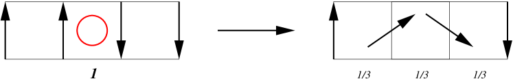
Figure 1: Illustration of vortex smearing: the $Z(2)$ links of the thin vortex plaquette (indicated by red circle) and the link rotation profile of the smeared (thick) vortex. Using steady rotations of $\pi/3$ in the same $U(1)$ subgroup, the center vortex flux $-\mathbbm{1}$ of the thin (dual) vortex plaquette is distributed uniformly within the original and neighboring plaquettes. This is indicated by the numbers below the plaquettes as multiples of $\pi$, indicating the composition of the total center vortex flux $\exp{i\pi}\equiv-\mathbbm{1}$. The $U(1)$ subgroup for each vortex plaquette is chosen such as to minimize the affected plaquettes.

There are of course many ways to implement these rotations, therefore we perform a systematic analysis to explore which method is best suited for our goal. In order to reproduce the original vortex structure the smoothed $SU(2)$ links should stay in the same hemisphere of the corresponding $S_{3}$ after MCG projection, hence we apply only rotations smaller than $\pi/2$. A statistical analysis shows that the maximally nontrivial plaquette reduces more effectively if the two corresponding links rotate in the same $U(1)$ subgroup of $SU(2)$, however the situation is nevertheless not trivial: It is interesting to observe that, overall, the smallest plaquette values are observed for link rotations of $\pi/5$ or $\pi/6$ away from their corresponding center elements, whereas for $\pi/3$ and $\pi/4$ we still observe plaquettes with Tr $U_{\mu\nu}=-2$. These situations can occur at vortex corners or intersections, where different rotations affect single plaquettes. In fact, we can easily construct situations where multiples of $\pi/3$ or $\pi/4$ add up to $\pm\pi$, resulting in $\exp{\pm i\pi}=-\mathbbm{1}$, see also Hollwieser:2012kb . For rotations up to $\pi/5$ MCG and center projection also reproduce the original vortex structure very well. If we now restrict all rotations to the same $U(1)$ subgroup, the smeared configurations still show a gap in the overlap spectra, i.e., no near-zero modes are found, as it is the case for maximal Abelian projected configurations. Therefore, we generalize the procedure; for each vortex plaquette we randomly choose a $U(1)$ subgroup to perform the smearing rotation. This way, the eigenvalue gap closes and a finite density of near-zero modes shows up. In order to improve the result, instead of randomly choosing the $U(1)$ subgroups we try to minimize the affected plaquettes. Now the maximally nontrivial plaquette reduces further, however the eigenvalue spectra do not change significantly. Finally, we try various smearing methods, i.e., APE, EXP, LOG and their improved and HYP versions Falcioni:1984ei ; Teper:1987wt ; Albanese:1987ds ; Morningstar:2003gk ; Hasenfratz:2007rf ; Durr:2007cy , to make the smeared vortex configurations even smoother. Even though the average plaquette now reduces further, intriguingly the maximally nontrivial plaquette moves back towards $-\mathbbm{1}$. While the standard smearing routines act too mildly, the improved ones, using bigger Wilson loops or the hypercubic nesting trick, smooth the configurations enough within a few smearing steps. In Fig. 2 we show the overlap and asqtad staggered spectra for original (full) $SU(2)$, MCG projected $Z(2)$ and various vortex and HYP smeared configurations. We see that 2-3 HYP smearing steps seem to be appropriate to reproduce the original Dirac spectra. However, even by systematically scanning the parameter sets for the various smearing routines, we cannot avoid that the vortex structure is deformed during the smearing and we are not able to reproduce the initial vortex configuration after MCG projection. Therefore we rule out standard smearing routines and try yet another strategy, i.e. distributing the vortex flux of a single vortex plaquette (Tr $U_{\mu\nu}=-2$) to several (neighboring) plaquettes.

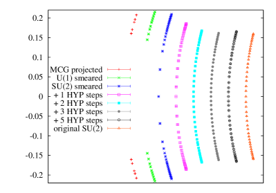
a) b)

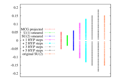
Figure 2: 20 lowest a) overlap and b) asqtad staggered eigenvalues for original (full) $SU(2)$, Maximal Center Gauge projected $Z(2)$, $U(1)$ and $SU(2)$ vortex smeared configurations with different numbers of HYP smearing steps.

II.2 Center vortex flux distribution

The first step is again to identify the vortex plaquettes, i.e. plaquettes with Tr $U_{\mu\nu}=2\exp{\pm i\pi}=-2$ in a given $Z(2)$ configuration. The plaquettes and therefore also the vortex structure are by definition gauge invariant. The $Z(2)$ links however are not and therefore the pair of links giving the overall $-\mathbbm{1}$ identified in the link smearing procedure discussed above is somewhat arbitrary. For the link rotation smearing we restricted ourselves to the direction of the jump from $+\mathbbm{1}$ to $-\mathbbm{1}$ (or the other way around) to perform the smooth rotation since this jump in fact defines the vortex in the $Z(2)$ configuration within its specific gauge. Thinking in terms of vortex flux distribution, however, there is no such preferred direction and we want to distribute the flux symmetrically among neighboring plaquettes. Therefore we now smear all four links of the vortex plaquette by individual link rotations in the same $U(1)$ subgroup in order to guarantee uniform flux distributions. The $U(1)$ subgroup is either chosen randomly for each vortex plaquette, or such as to reduce the plaquettes orthogonal to the vortex plaquettes, affected by the individual link rotations.

Fig. 3 shows an example of how to change the individual links using $\pm\pi/8$ rotations away from the original links. We have to distinguish four different cases according to the initial link configurations in order to get flux distributions of $\exp{\pm i\pi/2}$ and $\exp{\pm i\pi/8}$ at the original and four neighboring plaquettes summing up to the initial center element. The flux distributions for the individual cases are shown in Fig. 4. There are of course many ways to distribute the center vortex flux symmetrically and uniformly among various plaquettes, and even more ways to realize these distributions by different link configurations. In order to reproduce the initial vortex configuration however, we have to restrict the individual rotations to $\pm\pi/8$ giving the maximally possible center flux distribution shown in Fig. 4.

Smearing the $Z(2)$ configuration in this way (with individual rotations up to $\pm\pi/8$) is not enough to close the gap in the overlap spectrum. Standard smearing routines APE, EXP and LOG are again too mild to resolve this problem, whereas their improved HYP versions again destroy the vortex structure. Choosing the $U(1)$ subgroup for each of the four rotations individually in order to minimize the affected plaquettes, instead of applying the individual rotations to the four links in the same subgroup, not only destroys the uniform flux distribution but also does not close the gap in the overlap spectrum. Distributing the flux to more and more plaquettes dissolves the vortex structure in a sense, especially when it comes to edges and corners of the vortex structure. We therefore resort to yet a further technique: resolving the vortex structure within a finer lattice in order to generate more lattice spacings in which to smear it.

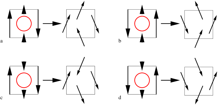
Figure 3: Distribution of center vortex flux: the $Z(2)$ links of the initial vortex plaquette ($\exp{\pm i\pi}=-\mathbbm{1}$) and the corresponding smeared links using $\pm\pi/8$ rotations away from the initial links. We distinguish four cases according to the initial link configurations. The smeared links distribute the flux as shown in Fig. 4, for rotations in the same $U(1)$ subgroup.

Figure 4: Vortex flux distributions for smeared vortex plaquettes with link rotations shown in Fig. 3. They add to a total flux of $\pm\pi$, consisting of $\pm\pi/2$ at the original vortex and $\pm\pi/8$ at neighboring plaquettes. These vortex flux distributions among plaquettes are valid for link rotations in the same $U(1)$ subgroup only, and do not necessarily correspond to the final vortex smeared configurations, where the individual rotations are performed in different $U(1)$ subgroups, such as to minimize the affected (including orthogonal) plaquettes, see text.

II.3 Vortex (lattice) refinement and blocking

By smearing the vortex structure on the original lattice we quickly end up destroying the vortex structure, since we cannot treat every single vortex edge, corner, writhing or intersection point, etc. independently. However, we can obtain more freedom in treating these structures by putting the vortex configuration on a finer lattice. For $Z(2)$ gauge links the refinement procedure can be defined straightforwardly and yields exactly the same vortex structure but on a finer lattice. The refinement procedure is illustrated in Fig. 5; we double the number of links in each direction, hence the lattice volume increases by a factor of $2^{4}=16$. If the initial link was $\mathbbm{1}$ we only insert two $\mathbbm{1}$ links, however if the initial link has value $-\mathbbm{1}$, we insert a $\mathbbm{1}$ and a $-\mathbbm{1}$ link in forward direction. The new link pairs are copied forward by half the initial lattice spacing in all orthogonal directions, e.g. an x-link $U_{x}(\vec{x})=-\mathbbm{1}$ at $\vec{x}=(x,y,z,t)$ gives $\tilde{U}_{x}=\mathbbm{1}$ at $(x,y,z,t)$, $(x,y+1/2,z,t)$, $(x,y,z+1/2,t)$, $\ldots$, $(x,y+1/2,z+1/2,t+1/2)$ and $\tilde{U}_{x}=-\mathbbm{1}$ at $(x+1/2,y,z,t)$, $(x+1/2,y+1/2,z,t)$, $(x+1/2,y,z+1/2,t)$, $\ldots$, $(x+1/2,y+1/2,z+1/2,t+1/2)$ .

Figure 5: Refinement routine: Example of one $-\mathbbm{1}$ (fat z-) link giving eight $-\mathbbm{1}$ and eight $\mathbbm{1}$ links after refinement.

Just as refinement gives the same vortex structure on the finer lattice, the inverse procedure, blocking, again gives the original configuration. During blocking, the copies between the coarse lattice planes are thrown away and the two refined links, e.g. $\tilde{U}_{x}(\vec{x}=(x,y,z,t))$ and $\tilde{U}_{x}(\vec{x}=(x+1/2,y,z,t))$, are multiplied to reproduce the original $U_{x}(\vec{x}=(x,y,z,t))=\mathbbm{1}\cdot\pm\mathbbm{1}=\pm\mathbbm{1}$ link, see also Sec. II.6 for more details. On the refined lattice, however, one now has the advantage that deformations of the vortex surface within the original lattice spacing still yield the correct vortex structure after blocking. Visualizing the actual (closed) vortex surface on the dual lattice, refinement not only multiplies the number of vortex plaquettes, yielding more (refined) plaquettes (and therefore also links) at e.g. vortex edges or corners, as shown in Fig. 6, but also adds links (and plaquettes) in directions orthogonal to the vortex surface, which we may use to smear our configurations. This way we may not make the vortex thicker in terms of the original lattice, but we can make the configuration smoother by adding additional rotations to the (refined) links or distributing the vortex flux to more (refined) plaquettes.

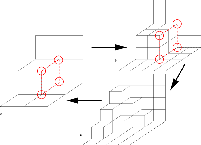
Figure 6: Vortex refinement (a$\rightarrow$b), smearing (b$\rightarrow$c) and blocking (c$\rightarrow$a): Example of a partial vortex surface on the dual lattice including edges and corners (red circles). Smearing the central (red dotted) plaquette in the coarse lattice (left) influences all other attached plaquettes since we smear in the directions orthogonal to the plaquette (i.e., its dual plaquette on the original lattice) and the vortex corners (and edges) are deformed. For the refined lattice on the right, smearing individual plaquettes only affects its direct neighbors if they are connected via an edge and therefore plaquettes attached to the vortex corners do not affect each other directly during smearing. Further, deformations of the refined vortex surface during smearing within the original lattice spacing (as indicated in c) will reproduce the original vortex structure after blocking.

The refinement and blocking procedures are discussed more extensively in Engelhardt:2000wc ; Bertle:2001xd where they help to remove ambiguities from vortex intersections, corners or writhing points, or, respectively, ultraviolet artifacts during vortex topological charge calculation. In fact, during vortex topological charge calculation the lattices are refined threefold, i.e., resulting in a lattice spacing $a/3$ in order to resolve intersection lines and to make sure that neighboring vortex surfaces cannot interact with each other. Even though smearing on finer and finer lattices might be more and more efficient, we restrict ourselves to a twofold refinement to limit the computational cost for the overlap Dirac operator evaluation. Nevertheless, resolving vortex structure ambiguities via refinement seems also useful for the present problem of smearing the vortex surface, since such structures, i.e., vortex intersections, corner or writhing points, are more easily deformed during the smearing process.

Having cast a configuration on a finer lattice, for the smearing routines we again start by identifying the (maximally nontrivial) center vortex plaquettes with Tr $U_{\mu\nu}=-2$. On the refined lattice there are of course more center vortex plaquettes compared to the original lattice. As mentioned above, the lattice volume, i.e., the number of lattice points and equally the number of links and plaquettes is multiplied by $2^{4}=16$. As can be seen in Fig. 5 however, the number of negative links is only increased by a factor of eight, since we also add eight positive links for an initially negative link. The number of vortex plaquettes finally is increased by four, as can be checked in Fig. 5 too, but can also be easily understood in terms of the dual lattice, where the vortex surface forms a closed surface of dual plaquettes, which are simply refined to four smaller plaquettes each (see also Fig. 6). We should therefore note that the vortex density is reduced by a factor four on the refined, original lattice; this ultimately was the initial goal of the refinement procedure, resolving vortex structure ambiguities by increasing the distance between close vortex structures or neighboring surfaces which would otherwise interact after thickening them during vortex smearing.

II.4 Refined link rotation smearing

As in section II.1, we locate the opposite link pairs causing (negative) vortex plaquettes now on the refined lattice and smooth out the jump from $\mathbbm{1}$ to $-\mathbbm{1}$ or the other way around. On the refined lattice we can extend the rotation to four links without disturbing any neighboring vortex plaquettes and additionally apply rotations to the neighboring links in link direction from the refinement procedure, see Fig. 7. We rotate the individual links either $\pi/8$ or $\pi/4$ away from their initial center elements and still reproduce the initial vortex configuration after blocking. At this stage, we made another interesting observation: Applying the Dirac operators to the refined, smeared configurations gives spurious results, the spectra show an even larger gap with individual eigenvalue bands, even for the asqtad staggered fermions. The problem seems related to the refinement procedure, since the asqtad (and the standard) staggered Dirac operator, which identifies zero modes well on center projected configurations, gives unphysical spectra already for the simply refined (non-smeared) configurations. This observation is insofar interesting as the refined lattices represent the same vortex configurations, except that they of course are half as thick compared to the original lattice due to the smaller lattice constant. The only difference to vortex configurations on originally finer lattices seems to be the fact that negative links only arise at every second (even) lattice slice of the corresponding link direction (e.g. x-links in x-slices, i.e., odd x-slices contain only $\mathbbm{1}$ x-links). Even though this seems not very likely in Monte Carlo generated vortex configurations, the fact that it causes a problem in identifying Dirac operator zero modes is worth noting. While the staggered Dirac operator might fail because of its even/odd-lattice implementation, we cannot think of any plausible explanation for the failure of the overlap Dirac operator. However, we find in the next section that this problem is not as severe for the overlap compared to the staggered fermions, since it is not present for the former in the case of flux distribution smearing on refined lattices, and therefore we will not discuss it further for now.

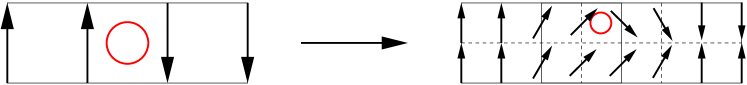
Figure 7: Refined link rotation smearing: The smearing rotation from $\mathbbm{1}$ to $-\mathbbm{1}$ can be extended to four links without disturbing any other vortex plaquettes. Center vortex plaquettes of the initial and refined (or MCG projected after smearing) configurations are again indicated by red circles. Link rotations in the top/bottom row are given by $\pi/8,\pi/4,3\pi/4,7\pi/8$ and $\pi/8,\pi/4,\pi/4,\pi/8$ and the individual $U(1)$ subgroups are chosen such that the affected plaquettes are minimized.

In order to overcome this issue in the present case of link rotation smearing, we try to spread the vortex structure back to its initial thickness, i.e., two lattice constants of the refined lattice, during the smearing process. Therefore we simply add another smeared link close to $-\mathbbm{1}$ to the corresponding odd lattice slice of the refined lattice. There are many different ways of doing the individual rotations; finally, we settle with the smearing rotations shown in Fig. 8, which seem to give the best results. The figure shows all rotations in the same U(1) subgroup, however, in practice, the subgroups for the individual rotations are chosen such as to minimize the corresponding plaquettes, i.e., reduce the maximally nontrivial plaquette among the six plaquettes affected by the link being rotated as much as possible. In order to check the vortex flux distribution among the refined and smeared plaquettes, we analyze the idealized case of all rotations in one $U(1)$ subgroup, which of course is not the optimal case for the overall smearing routine. We restrict ourselves to the plaquettes in one plane only, cf. Fig. 9, noting however that the smearing routine distributes vortex flux also to orthogonal plaquettes. The center vortex flux distribution is shown in Fig. 9 in terms of fractions of $\pi$ for the individual refined and original plaquette values for the two cases plotted in Fig. 8, i.e., $\mathbbm{1}\rightarrow-\mathbbm{1}$ or $-\mathbbm{1}\rightarrow\mathbbm{1}$. The individual contributions add up to $\pm\pi$ respectively, giving a flux of $\pm\pi/2$ for the initial vortex plaquette and $\pm\pi/4$ for the neighboring plaquettes.

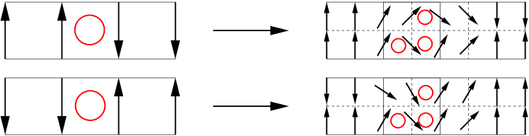
Figure 8: Refined link rotation smearing for $\mathbbm{1}\rightarrow-\mathbbm{1}$ and $-\mathbbm{1}\rightarrow\mathbbm{1}$ link pairs. The individual $U(1)$ rotations of the links from left to right in the top and bottom rows of the two cases are given by $\pi/8,\pi/4,5\pi/8,3\pi/4;\pi/8,3\pi/4,\pi/8,\pi/4$ and $5\pi/8,7\pi/8,\pi/8,\pi/8;\pi/8,3\pi/4,\pi/8,\pi/4$. The odd (lower) lattice slices also contain a certain number of smeared links close to $-\mathbbm{1}$, introducing additional vortex plaquettes (red circles) which distort and therefore smear the vortex surface in link direction. The $U(1)$ subgroups are not the same for the individual rotations, but chosen such as to minimize the corresponding plaquettes.

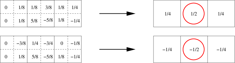
Figure 9: Vortex flux distributions for refined link rotation smeared vortex plaquettes with $\mathbbm{1}\rightarrow-\mathbbm{1}$ and $-\mathbbm{1}\rightarrow\mathbbm{1}$ link pairs in terms of fractions of $\pm\pi$ adding up to a total flux of $\pm\pi$, with $\pm\pi/2$ at the original vortex and $\pm\pi/4$ for neighboring plaquettes. These vortex flux distributions among plaquettes are valid for link rotations in the same U(1) subgroups only, and do not necessarily correspond to the final vortex smeared configurations, where the individual rotations are chosen such as to minimize the corresponding plaquettes.

With this refined smearing procedure, a flat vortex surface is distorted within the initial thickness it had before the refinement procedure, which seems to work just like a smearing effect for the thick center vortices. In terms of the thin vortex structure, i.e., if we apply the MCG and project the smeared (thick) vortices back to $Z(2)$, the thin vortex exhibits a rough instead of a flat surface, since we introduced additional vortex plaquettes on the refined lattice, within the original thickness of the vortex (see also Fig. 8). The actual effect of this vortex surface distortion will be presented for classical, i.e., planar and spherical vortices in section IV. These additional plaquettes are of course removed after blocking and we recover the original vortex surface. They are also partially removed already on the refined lattice by the smoothing procedure discussed in the next section.

II.5 Refined vortex flux smearing

On the refined lattice, we have a straightforward way to distribute the center vortex flux among the four refined plaquettes corresponding to each initial center vortex plaquette without affecting neighboring plaquettes or even links. In Fig. 10 we show examples of link configurations to distribute the center vortex flux $\exp{i\pi}=\exp{-i\pi}=-\mathbbm{1}$ uniformly among the four refined plaquettes, each carrying one fourth of the initial center vortex flux. The uniform distribution is of course only guaranteed if we apply all link rotations of $\pm\pi/4$ and $\pi/2$ in the same $U(1)$ subgroup.

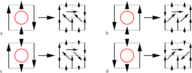
Figure 10: Examples of link configurations giving uniform center vortex flux distribution among the four refined plaquettes of the initial center vortex plaquette. The individual link rotations are given by $+\pi/2$, $\pm\pi/4$ and $\pm 3\pi/4$ in the same $U(1)$ subgroup. Each refined plaquette carries one fourth of the initial center vortex flux; a),c) $\exp{i\pi}=-\mathbbm{1}$ and b),d) $\exp{-i\pi}=-\mathbbm{1}$. In order to minimize the orthogonal plaquettes (the ones orthogonal to the displayed plane) we vary the $U(1)$ subgroup by applying ”2D gauge transformations” (see text) at the central points of the plaquettes, indicated by the red circle.

Since we change only links at half the initial lattice spacings, i.e., links dividing the original plaquettes into four refined plaquettes, blocking trivially (the mentioned links are thrown away) restores the initial $Z(2)$ link configuration and therefore the original vortex structure. However, this method also changes links orthogonal to the links giving the initial jump from $\mathbbm{1}$ to $-\mathbbm{1}$ or vice versa. In fact these are the links in direction of the jump (or, rotation, after smearing) plotted in Fig. 10 with rotations of $\pm\pi/4$. Depending on the vortex structure, the plotted link configurations may still cause maximally nontrivial plaquettes in directions orthogonal to the displayed plane; as mentioned above, we can easily construct situations where $\pm\pi/4$ and $\pi/2$ links add up to $\pm\pi$, giving $\exp{\pm i\pi}=-\mathbbm{1}$ for a plaquette. Therefore, we try to ”2D gauge transform” away from the simple examples in Fig. 10. In fact, applying a gauge transformation at the central lattice site leads to arbitrary link configurations without changing the plaquettes in the displayed plane. Since we only want to affect the displayed links and not the ones orthogonal to the displayed (paper) plane, we do not apply real (4D) gauge transformations, affecting all links at a certain point, but restrict the transformations to the displayed links in the 2D plane. Using this ”2D gauge transformation” at the central points of the original vortex plaquettes, using random $SU(2)$ vectors, we can minimize the affected plaquettes orthogonal to the original or refined vortex plaquette. This way we eliminate maximally nontrivial plaquettes and the overlap fermions seem to detect zero modes properly. Staggered fermions, however, still show a gap, which might be related to the problem discussed in the last section, i.e., its even/odd lattice implementation and the refinement procedure. In fact, the smeared configurations shown in Fig. 10 all have nontrivial links in the even (upper) slice of the refined lattice. Since we apply the ”2D gauge transformation” in order to minimize the plaquettes, the link configuration we start with does not matter. However, if we analyze the refined flux smeared configurations, we find that the majority of links close to $-\mathbbm{1}$ is still found in the even lattice slices after the smearing routine. This seems to be reasonable, since after refinement $-\mathbbm{1}$ links only appear in even lattice slices, see also Fig. 5; links close to $-\mathbbm{1}$ in odd lattice slices would obviously lead to plaquettes close to $-\mathbbm{1}$ as well, which we try to avoid. By omitting the minimizing ”2D gauge transformation” and applying different link rotations in order to reproduce the uniform flux distribution among the plaquettes we may overcome the problem of the staggered Dirac operator in a similar way as in the previous section. However, even though we examined many different combinations of link rotations, we did not find a solution which gives equally good results for both, overlap and staggered fermions. We also attempted extending the flux distribution to the next neighboring plaquettes, and further also included ”2D gauge transformations” at the points next to the central point. Apart from not being able to solve the initial problem this way, we furthermore lose the vortex finding property. Therefore we settle on the link configurations shown in Fig. 10, supplemented by the ”2D gauge configuration” at the center of the original vortex plaquette. This method gives us the best results towards our goal, approaching continuum $SU(2)$ gauge dynamics, except for the staggered fermion spectra. These, however, can be improved with yet another, final step in our vortex smearing procedure, described in the next section.

II.6 Vortex smeared blocking

A simple way to eliminate ultraviolet fluctuations of the center projection vortices obtained in the maximal center gauge is to apply blocking steps such as to transfer the vortex configurations onto new coarser lattices, while always preserving their chromomagnetic flux content on length scales larger than the new lattice spacing. Consider a new coarse lattice with $n$ times the spacing of an old fine lattice, superimposed on the latter such that all sites of the coarse lattice coincide with sites of the fine lattice. In this work we use $n=2$, but the blocking procedure in principle is feasible for arbitrary $n$. The gauge phases associated with plaquettes on the coarse lattice then are defined to be equal to the $n\times n$ Wilson loops on the old fine lattice to which these plaquettes correspond. Equivalently, if an odd number of vortices pierces the $n\times n$ Wilson loop on the old fine lattice, then one vortex is defined to pierce the corresponding plaquette on the new coarse lattice; if an even number of vortices pierces the $n\times n$ Wilson loop on the fine lattice, then no vortex pierces the corresponding plaquette on the coarse lattice. Note that, thinking in terms of thin center vortices, i.e., a $Z(2)$ lattice, this argumentation and the blocking simply reduces to the multiplication of the $n^{2}$ plaquettes forming the $n\times n$ Wilson loop. Note also that blocking manifestly preserves the values of all Wilson loops (as far as they can still be defined on the coarse lattice). Thus, blocking leaves the string tension induced by a thin vortex ensemble invariant. The only information that is lost during blocking are the original small plaquettes, i.e., ultraviolet fluctuations.

Now, in terms of $Z(2)$ lattices, we have seen that blocking is the exact inverse procedure to refinement. Hence, blocking a refined lattice exactly gives us the same links and plaquettes present in the original lattice, and therefore also the same vortex structure. For the following discussion let us identify original (x,y,z,t) and refined lattice sites (2x-1,2y-1,2z-1,2t-1), and let us call the latter ”odd” lattice sites on the refined lattice, since all indices are odd. Whenever one index of a refined lattice site is even, the lattice site is not part of the original lattice and we may call it ”half-even” or ”even” if all indices are even. It now is interesting to note that, due to the refinement procedure we defined in section II.3, we can alternatively block the refined lattices starting at (half-)even (refined) lattice points, i.e., one refined (half an original) lattice spacing away from the original (odd refined) lattice sites in any forward space-time direction and still get back the exact, original configuration. Hence, instead of starting the blocking procedure at the (odd) refined lattice point (1,1,1,1), which actually coincides with (1,1,1,1) on the original lattice, we can also start blocking at, e.g., point (2,1,1,1) on the refined lattice to reproduce the original configuration, or even at (2,2,2,2) as shown in Fig. 11. Now, as mentioned before for the refined flux smearing procedure, blocking the smeared lattice starting at odd refined lattice sites recovers the original vortex configurations, as the links making up the original plaquettes are not changed during the smearing procedure. However, if we start the blocking at any (half-)even lattice site we have to multiply several smeared $SU(2)$ links instead of $\pm\mathbbm{1}$s and end up with a $SU(2)$ instead of a $Z(2)$ configuration. This new, blocked configuration now represents some smeared version of the original $Z(2)$ lattice, since the smeared links are derived from the original lattice after refinement. In order to keep the smearing procedure symmetric, i.e., we do not want to favor any smearing direction, we start the blocking procedure at the even lattice sites of the refined lattice, i.e. one refined (half an original) lattice spacing forward in every space-time direction, as indicated in Fig. 11 by the red arrow. This procedure we will call ”smeared blocking” in the following.

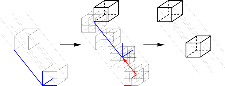
Figure 11: Refinement and smeared blocking procedure: After refinement the blocking is not performed starting at (1,1,1,1), the lower, left corner, but half an original (i.e., one refined) lattice spacing forward in every space-time direction, i.e., (2,2,2,2) on the refined lattice, indicated by the red arrow (the time direction is indicated by the fine lines connecting the space-like cubes). Without vortex smearing between steps 2 and 3 the lattices before and after the whole procedure are actually the same; with vortex smearing the re-blocked lattice gives a smeared version of the original lattice.

II.7 Vortex smoothing

Since center projection vortices exhibit artificial ultraviolet fluctuations, we also use the smoothing procedure first discussed in Bertle:1999tw . It operates using elementary cube transformations on the lattice vortex surface such that a net decrease in the number of vortex plaquettes is achieved.

One point at which the smoothing procedure can be applied is before the refinement process; note that, after refining, the vortex surface smoothing has no effect any more, since elementary cubes are made up of eight smaller cubes after refinement. The initial idea was that smearing smoothed vortex configurations might be easier since the number of small vortex structures is reduced. However, we found that results for smeared original and smoothed vortex configurations, even though they might differ for individual configurations, agree within uncertainties in ensemble averages. In fact, it was shown in Bertle:1999tw that smoothing does not change the long-range physics of gauge configurations, since it only removes artificial ultraviolet fluctuations of the vortices.

On the other hand, smoothing does turn out to be useful at a different point; namely, for our artificially distorted vortex surfaces after refined smearing and MCG projection, since it removes those distortions which turn out to be only elementary cube transformations of the refined vortex configurations. However, the smoothing procedure does not necessarily reproduce the originally refined vortex configuration, it only gives a smooth version of the vortex surface within the original lattice spacing (two refined lattice spacings). Again, see section IV for more details on the distortion and smoothing effects on classical configurations.

II.8 Summary

To conclude this section we briefly summarize the vortex smearing method for $Z(2)$ configurations (the initial smoothing and final blocking are optional and therefore put in parentheses):

• (smoothing of the thin vortex surface, see Sec. II.7 for details)

• refinement of the $Z(2)$ lattice configuration, see Fig. 5

• identification of vortex plaquettes, i.e., plaquettes with Tr $U_{\mu\nu}=-2$

• application of one of the two smearing routines:

  • link rotation smearing:

    • identification of opposite links causing the overall $-\mathbbm{1}$ of the plaquette, i.e., $U_{\mu}(\vec{x})U_{\mu}(\vec{x}+\hat{\nu})$ or $U_{\nu}(\vec{x})U_{\nu}(\vec{x}+\hat{\mu})$

    • application of refined link rotation smearing as depicted in Fig. 8, except for the $U(1)$ subgroups of the individual rotations not chosen uniformly, but such as to minimize the affected plaquettes

  • application of the refined vortex flux smearing, as depicted in Fig. 10, including ”2D gauge transformations” in order to minimize the orthogonal plaquettes (see Sec. II.5 for details)

• (vortex smeared blocking, see Fig. 11)

III Results

In order to test our method we use 500 thermalized Lüscher-Weisz $SU(2)$ gauge field configurations on $8^{4}$ lattices at coupling $\beta=3.3$ which gives a lattice string tension $\sigma_{lat}=0.1112\pm 0.0017$ corresponding to a lattice spacing $a=0.1495\pm 0.0012$fm. The locations of center vortices are identified as usual by mapping the $SU(2)$ lattice to a $Z(2)$ lattice which contains, by definition, only thin vortex excitations. The mapping is carried out by fixing the lattice to the direct maximal center gauge, which is equivalent to Landau gauge in the adjoint representation, and which maximizes the squared trace of the link variables. The gauge-fixing procedure is the over-relaxation method. We also apply the above mentioned vortex smoothing and evaluate our results on both original and smoothed vortex configurations after vortex smearing. As mentioned above, the results for original and smoothed vortex configurations are equal within uncertainties of ensemble averages. Hence, by combining the results we can double our statistics - we may think of two different Gribov copies for each Monte Carlo configuration, although the vortex structures are of course correlated. In the following sections we present various observables for refined link rotation smeared, refined vortex flux smeared and their vortex smeared blocked configurations and discuss the individual advantages and drawbacks.

III.1 Fermionic Eigenvalues and Overlap zero modes

Fermion eigenmodes are calculated by an implementation of the MILC milc code at the Phoenix and Vienna Scientific Cluster (VSC) of the Vienna University of Technology (VUT) and the Riddler Cluster at New Mexico State University (NMSU). In Fig. 12 we display the twenty lowest-lying complex conjugate eigenvalue pairs of the overlap and asqtad staggered Dirac operators  Narayanan:1994gw ; Neuberger:1997fp , for center projected, vortex smeared and original configurations. For the spectra on the refined lattices, the eigenvalues are multiplied by a factor two, to account for the refinement effect: For the free Dirac operator, using a plane wave ansatz $\psi_{\alpha}(x)=u_{\alpha}\ \exp(ip_{\mu}x_{\mu})$, the eigenvalues are given by $\lambda\propto\sqrt{p_{\mu}p_{\mu}}$, see e.g. Hollwieser:2013xja . The allowed values for $p_{\mu}$ are

$$p_{i}=\frac{2n_{i}\pi}{aN_{S}},\quad\quad p_{4}=\begin{cases}\frac{2n_{4}\pi}{aN_{T}}&\mbox{for periodic BC}\\ \frac{(2n_{4}+1)\pi}{aN_{T}}&\mbox{for anti-periodic BC}\end{cases},\quad\quad n\in\mathbb{Z}\,,$$

with $N_{S}$ the spatial and $N_{T}$ the temporal extent of the lattice. Hence, even though there are $2^{4}=16$ times more eigenmodes on the refined lattice, the eigenvalues scale linearly with $1/N_{S,T}$. The seeming mismatch is of course compensated by much higher degeneracy of higher modes on the finer lattice.

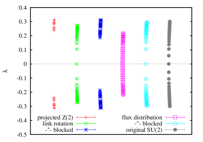
a) b)

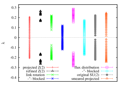
Figure 12: 20 lowest a) overlap and b) asqtad staggered eigenvalues for original (full) $SU(2)$, Maximal Center Gauge projected $Z(2)$ and vortex smeared configurations.

Looking more closely at the overlap spectra, we see that there only appear to be five eigenvalue pairs (out of twenty) in the center projected case, indicating a four-fold degeneracy when the overlap operator is applied to $Z(2)$ lattice configurations. This factor of four has the following origin: In the first place, when link variables are simply plus or minus the $2\times 2$ identity matrix, the two colors decouple, and we have a factor of two degeneracy. Secondly, whenever the link variables are real and the Dirac operator has the Wilson or overlap (but not staggered) form, the eigenvalue equation $D\psi_{n}=\lambda_{n}\psi_{n}$ is invariant under charge conjugation. Thus, if $\psi_{n}$ is an eigenstate with eigenvalue $\lambda_{n}$, then $C^{-1}\psi_{n}^{*}$ is also an eigenstate, with the same eigenvalue Leutwyler:1992yt . This gives another factor of two, resulting in an overall four-fold degeneracy. For the vortex smeared configurations there is no such degeneracy and the spectra approach the original (full) $SU(2)$ spectra. The actual correspondence of the spectra can be seen in the scatter plots in Fig. 13 for the ensemble mean eigenvalues and in Fig. 14a) for the overlap eigenvalues on individual configurations. The asqtad staggered results are not as good as for the overlap Dirac operator in the sense that the gap is much larger than for the original configurations, see Fig. 12b. This large gap is caused by the refinement procedure, as discussed already in Sec. II.4. Smearing the refined $Z(2)$ configurations still shows large eigenvalue gaps which only go away after smeared blocking. Since we focus on topological properties and therefore especially on zero modes, the smearing routine was optimized to reproduce the best overlap results. In Fig. 12b) we also plot the asqtad staggered spectra for simply refined and vortex smeared + MCG projected $Z(2)$ configurations; while the naive refinement process (without smearing) obviously troubles the Dirac operators (the overlap response is similar), the latter actually reproduces spectra which somewhat seem to interpolate between the original and projected cases. In Fig.14b) we show a scatter plot of the number of zero modes for original (full) $SU(2)$ and vortex smeared configurations. There is no one-to-one correlation for the individual configurations; the reason for this will be discussed in the next section where we analyze the influence of our method on topological properties of the gauge field.

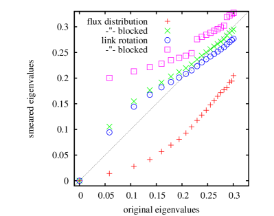
a) b)

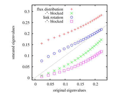
Figure 13: Scatter plot of a) overlap and b) asqtad staggered non-zero eigenvalues for original (full) $SU(2)$ and vortex smeared configurations (ensemble mean eigenvalues).

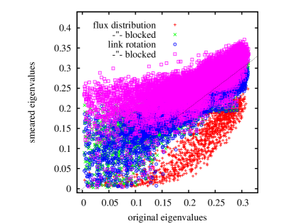
a) b)

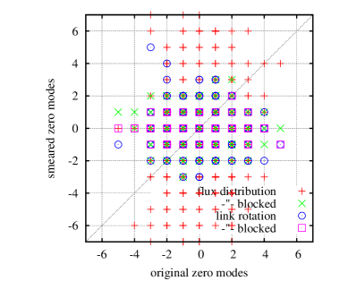
Figure 14: Scatter plot of overlap a) non-zero eigenvalues and b) number of zero modes for individual configurations.

Before that, we look at the distributions of the ”unfolded” level spacing and the lowest (non-zero) eigenvalues. Chiral random matrix theory (RMT) predicts that these distributions are universal when they are classified according to symmetry properties of the Dirac operator and the sector of fixed topological charge under consideration BerbenniBitsch:1997tx ; Edwards:1999ra ; Verbaarschot:2000dy . Fermion modes in the fundamental representation of gauge group SU(N) of the overlap operator have the symmetry properties of the orthogonal ensemble, i.e. their distribution is described by a Gaussian measure on the space of real $N\times N$ symmetric matrices and is invariant under orthogonal conjugation, whereas for the staggered operator they fall into the symplectic ensemble, described by a Gaussian measure on the space of quaternionic $N\times N$ Hermitian matrices and its distribution is invariant under conjugation by the symplectic group.

The unfolding is done by first sorting all non-zero positive eigenvalues $\lambda_{i}^{n}$ with $n$ labeling the configuration number in ascending order. $N_{i}^{n}$ then gives the location of $\lambda_{i}^{n}$ in the sorted list and is referred to as the unfolded spectrum. The level spacing $s$ is simply given by $s=(N_{i+1}^{n}-N_{i}^{n})/N_{c}$ where $N_{c}$ is the number of configurations. The distributions of the unfolded level spacing $s$ in RMT are well approximated by the various Wigner distributions Halasz:1995vd

$$P(s)=\begin{cases}{\pi\over 2}s{\rm e}^{-{\pi\over 4}s^{2}}&\mbox{orthogonal ensemble}\cr{262144\over 729\pi^{3}}s^{4}{\rm e}^{-{64\over 9\pi}s^{2}}&\mbox{symplectic ensemble}.\end{cases}$$ (1)

In Fig. 15a) we show the distribution of the unfolded level spacing for overlap and staggered fermions on our original $SU(2)$ configurations. The distributions are slightly shifted to lower values compared to RMT predictions, the reason could be a lack of statistics and our rather small lattice volume, but more likely our choice of gauge coupling $\beta=3.3$, which is right at the deconfinement phase transition where fluctuations can be expected. Fig. 15b) shows the results for overlap fermions on original and smeared configurations and we observe that the smearing processes shift the distributions further to the left, i.e. smaller level spacings. Only the blocking procedure for link rotation smearing seems to strongly distort the level spacing distributions. The results for staggered fermions are presented in Fig. 16, smearing again shifts the distributions slightly to smaller level spacings, after blocking, however, smeared and original distributions are not further apart than original and RMT predictions.

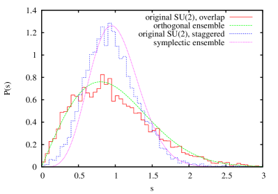
a) b)

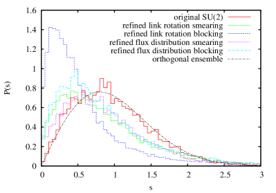
Figure 15: Distribution of the ”unfolded” level spacing $s$ for a) overlap and staggered eigenvalues on original configurations versus RMT universality predictions and b) overlap eigenvalues on original and smeared configurations. For better differentiation we attach the individual plots in Fig. 31 in Appendix A.

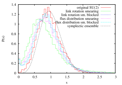
a) b)

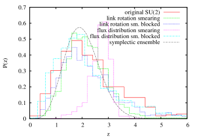
Figure 16: a) Distribution of the ”unfolded” level spacing $s$ for staggered eigenvalues on original and smeared configurations. b) Distribution of the smallest staggered eigenvalue $\lambda_{min}$ and RMT universality prediction $P(z)$ versus the rescaled variable $z=\Sigma V\lambda_{min}$, where $V$ is the volume and $\Sigma$ is the infinite volume value of the chiral condensate. Fitted values for $\Sigma$ are given in Table 1. For better differentiation we attach the individual plots in Figs. 34,35 in Appendix B.

Next we look at the distribution of the lowest eigenvalue $\lambda_{\rm min}$ for the various ensembles. Chiral RMT predicts that these distributions are universal when they are classified according to the number of exact zero modes $\nu$ within each ensemble and then considered as functions of the rescaled variable $z=\Sigma V\lambda_{\rm min}$. Here $V$ is the volume and $\Sigma$ is the infinite volume value of the chiral condensate $\langle\bar{\psi}\psi\rangle$. RMT gives for the distribution of the rescaled lowest eigenvalue for the orthogonal ensemble, expected to apply to the overlap fermions, in the $\nu=0$ and $\nu=1$ sector Forrester:1993kf

$$P(z)=\begin{cases}{2+z\over 4}{\rm e}^{-{z\over 2}-{z^{2}\over 8}}&\mbox{if $\nu=0$}\cr{z\over 4}{\rm e}^{-{z^{2}\over 8}}&\mbox{if $\nu=1$}.\end{cases}$$ (2)

For the symplectic ensemble, expected to apply to the staggered fermions, the RMT prediction is Forrester:1993kf ; Nagao:1995np ; Nagao:1998np

$$P(z)=\begin{cases}\sqrt{\pi\over 2}z^{3/2}I_{3/2}(z)e^{-{z^{2}\over 2}}&\mbox{if $\nu=0$}\cr{2\over{(2\nu+1)!(2\nu+3)!}}z^{4\nu+3}{\rm e}^{-z^{2}\over 2}T_{\nu}(z^{2})&\mbox{if $\nu>0$},\end{cases}$$ (3)

where $I_{3/2}(z)$ is the modified Bessel function and $T_{\nu}(x)$ a rapidly converging series based on partitions of integers, specified in the references. Staggered fermions, however, do not have exact zero modes at finite lattice spacing, even for topologically non-zero backgrounds, and thus seem to probe the $\nu=0$ predictions of chiral random matrix theory only. We compare the RMT predictions with our data in Fig. 16b) for staggered and Fig. 17 for overlap fermions. If one knows the value of the chiral condensate in the infinite volume limit, $\Sigma$, the RMT predictions for $P(z)$ are parameter free. On the rather small systems that we considered here, we did not obtain direct estimates of $\Sigma$. Instead, we made one-parameter fits of the measured distributions to the RMT predictions, with $\Sigma$ the free parameter and results given in Table 1. We note that the chiral condensate is very small and results on the various ensembles vary, within rather large uncertainties caused by small statistics and also the choice of gauge coupling $\beta=3.3$ right at the deconfinement phase transition causing large fluctuations. The distributions of the lowest staggered eigenvalues in Fig. 16b) are not consistent with RMT predictions for the original configurations; after link rotation smearing, they actually seem to agree with RMT predictions, but not for flux distribution smearing. After blocking the original distributions are reproduced, for different fitting parameters, i.e. chiral condensates though. Finally, the overlap results shown in Fig. 17 for $\nu=0$ and $\nu=1$ sectors are broadly consistent with RMT predictions, with the exception of link rotation smeared blocking in the $\nu=0$ case, which deviates strongly from the other distributions, and a somewhat distorted distribution for flux distribution smearing (without blocking) in the $\nu=1$ case. For $\nu=0$ the distribution found in the original configurations differs at zero eigenvalue from the RMT prediction, i.e., we find less low-lying eigenmodes. We conclude that the smeared ensembles roughly reproduce Dirac spectra and distributions of the original configurations except for link rotation smeared blocking with overlap and flux distribution smearing with staggered fermions.

a) b)

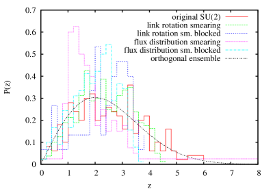
Figure 17: Distribution of the smallest overlap eigenvalue $\lambda_{min}$ and RMT universality prediction $P(z)$ for topological sectors a) $\nu=0$ and b) $\nu=1$ versus the rescaled variable $z=\Sigma V\lambda_{min}$, where $V$ is the volume and $\Sigma$ is the infinite volume value of the chiral condensate. Fitted values for $\Sigma$ are given in Table 1. Find the individual plots in Fig. 32,33 in Appendix A.

Configuration	overlap, $\nu=0$	overlap, $\nu=1$	staggered
original $SU(2)$	0.018 (133)	0.014 (255)	0.016 (500)
link rotation smeared	0.017 (341)	0.011 (393)	0.016 (1000)
-”- blocked	0.011 (928)	0.014 (66)	0.015 (1000)
flux distribution smeared	0.011 (87)	0.010 (174)	0.008 (1000)
-”- blocked	0.013 (480)	0.014 (444)	0.017 (1000)

Table 1: The chiral condensate $\Sigma$ from fits of the distribution of the lowest eigenvalue to the RMT predictions and the number of configurations in each topological sector in parenthesis.

III.2 Gluonic and Fermionic Topological Charge Correlation

If we want to recover the topological structure of the original (full) SU(2) configurations from the vortex smeared configurations we face the problem that standard gluonic definitions of topological charge via plaquette or hypercube constructions need some smearing or cooling procedure in order to guarantee a smooth gauge background which fulfills the Lüscher condition Luscher:1981zq . However, smoothing and especially cooling destroys the relevant vortex structures. In a word, gluonic topological charge definitions are not very reliable in the background of center vortices, this was also discussed in Hollwieser:2012kb . For the gluonic topological charge $Q_{T}$ we use the integral (sum, on the lattice) of the gluonic charge density $q(x)=\frac{1}{16\pi^{2}}\,\mathrm{tr}(\mathcal{F}_{\mu\nu}\tilde{\mathcal{F}}_{\mu\nu})$ in the “plaquette” and/or “hypercube” definitions on the lattice DiVecchia:1981qi ; DiVecchia:1981hh , which in fact give almost the same results, see Fig. 18a). In Fig. 18b) we show that the gluonic topological charge after cooling or LOG smearing correlates very well on both, original and vortex smeared configurations.

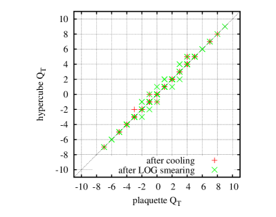
a) b)

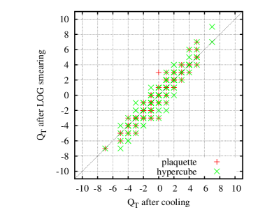
Figure 18: a) Scatter plot of plaquette and hypercubic definition of topological charge $Q_{T}$ after cooling and LOG smearing. b) Scatter plot of $Q_{T}$ after cooling and LOG smearing for plaquette and hypercube definitions. Both plots are for vortex smeared configurations, for original (full) configurations they look very similar.

The Atiyah-Singer index theorem relates the number of exact fermionic zero modes of a configuration and the topological charge $Q_{F}=\mbox{Tr}(\gamma_{5}D_{ov})=n_{-}-n_{+}=\text{ind}D_{ov}$ Atiyah:1971rm , which we call the fermionic topological charge. The relation $Q_{T}\approx Q_{F}$ is not exact on either original or vortex smeared configurations, see Fig. 19 for topological charge correlation between the two definitions on individual configurations. These results are not affected by additional cooling or LOG smearing. In view of the above concerns, it is not surprising that the correlation of either fermionic $Q_{F}$ (as seen in Fig. 14b) or gluonic topological charge $Q_{T}$ of the vortex smeared configurations with the original topological charge is not very good. In Fig. 19 we see that the refined vortex smeared configurations overestimate the original topological charge. For the smeared blocked configurations the net topological charge $Q_{T}$ is comparable to the original one; actually, in the blocked vortex flux distribution smeared case one can see a slightly positive correlation, see Fig. 20b. However the correlation between individual configurations is not very good. Again, this is not very surprising since cooling or smearing in order to evaluate the gluonic topological charge on the lattice destroys its center vortex content. However, in Bertle:2001xd it was shown that the vortex topological charge defined there based directly on the structure of the vortex configurations gives a good estimate of the topological susceptibility of the gauge field ensemble. Therefore we analyze the vortex topological charge and the topological susceptibility next.

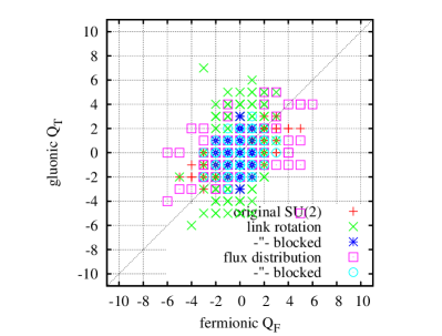
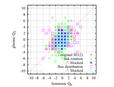
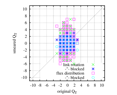
a) b) c) d)

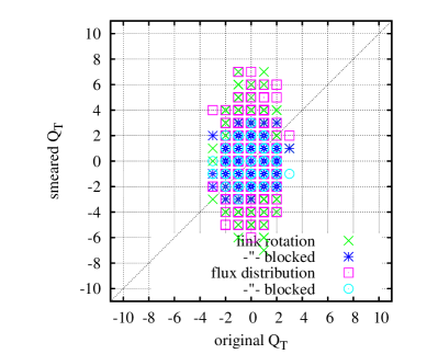
Figure 19: Scatter plot of fermionic $Q_{F}$ and gluonic topological charge $Q_{T}$ after a) cooling or b) (LOG) smearing on original (full) $SU(2)$ and various vortex smeared configurations ($Q_{F/T}$ on same configs); Scatter plot of gluonic topological charge $Q_{T}$ after c) cooling and d) (LOG) smearing for original (full) vs. vortex smeared configurations. In the blocked vortex flux distribution smeared case one can actually see a positive correlation, see also Fig. 20.

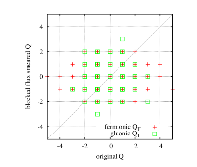
a) b)

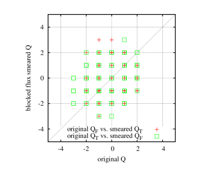
Figure 20: Scatter plot of fermionic and gluonic topological charge correlations and cross-correlations between original (full) vs. blocked vortex flux distribution smeared configurations.

III.3 Vortex Topological Charge and Topological Susceptibility

Center vortices give rise to topological charge at intersection and writhing points Engelhardt:2000wc ; Engelhardt:2002qs . It is known from Bertle:2001xd that center vortices reproduce the topological susceptibility of the original gauge fields. We want to estimate how well our vortex smearing procedure recovers this effect and further, how accurately the vortex topological charge reveals the topological content of individual gauge fields, i.e., we are interested in the correlation of the vortex topological charge with the index and gluonic topological charge definitions. The concepts of blocking and smoothing were introduced in Sec. II.7 and II.6, for more details on the use of these methods during vortex topological charge calculation see Bertle:2001xd , where it was also shown that the string tension is rather independent of vortex smoothing; however, smoothing reduces vortex topological charge and susceptibility by removing short range fluctuations of the vortex structure. On our original $8^{4}$ lattices with lattice spacing $a\approx 0.15$fm 1-2 blocking steps seem appropriate during the vortex topological charge calculation in order to get in the range of a physical vortex thickness of $~{}0.4$fm DelDebbio:1996mh ; DelDebbio:1998uu ; Engelhardt:1998wu . The refined lattices should accordingly be blocked 2-3 times.

The vortex topological charge is not necessarily correlated to the index of the Dirac operator, since the vortex configurations do not represent a topological torus, as there are monopoles and Dirac strings present. Thus, the basic index theorem is not valid and extra terms appear which are reflected in the difference of the vortex topological charge and the index. During cooling or smearing, monopoles and Dirac strings are smoothed out or fall through the lattice and the toroidal topology is restored, hence $F\tilde{F}$ approaches the index topological charge. However, the vortex finding property is lost during smearing and the vortex topological charge quickly vanishes for full configurations. These aspects were discussed in more detail in Hollwieser:2012kb . Vortex topological charge depends on the orientation of the (thick) vortex surfaces. The (thin) $Z(2)$ vortices lack any information of orientation and in order to calculate the vortex topological charge, orientation is applied randomly to the vortex surfaces. Similarly, during vortex smearing, by replacing the ”$Z(2)$ jump” with a smooth, random rotation in the $SU(2)$ space, we automatically give the vortex surfaces a random orientation in the color space, which influences the gluonic topological charge. Since these two processes are independent, we can not expect that the smeared vortex configurations or the vortex topological charge in general give comparable results for individual configurations concerning topological properties. However, as stated at the beginning of this section, the topological susceptibility of original gauge fields is mirrored by the vortex topological charge. Hence, we want to verify if this is also true for the vortex smeared configurations and if we can reproduce the topological susceptibility of the original $SU(2)$ gauge fields. The vortex topological charge for original and smeared configurations is essentially the same, since we deal with identical vortex structures. However, the random application of vortex orientation ruins a one-to-one correlation, unless we use the same random generator every single time. Even though this random step has no influence on the rather dominant writhing point contribution to topological charge, the random contribution of a few intersection points is enough to destroy a one-to-one correlation between individual configurations. Taking together all arguments from the previous and this section concerning the different approaches to topological charge determination, from center vortices, gluonic or fermionic definitions, it is not surprising that the first of these does not exactly reproduce the latter ones for individual configurations. In Figs. 21 and 22 we show correlations between gluonic resp. fermionic and vortex topological charge - there is no one-to-one correlation.

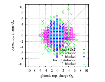
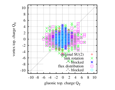
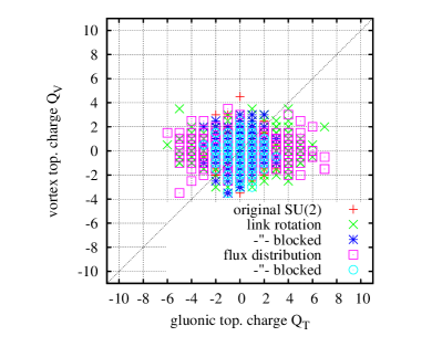
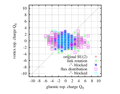
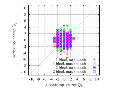
a) b) c) d) e) f)

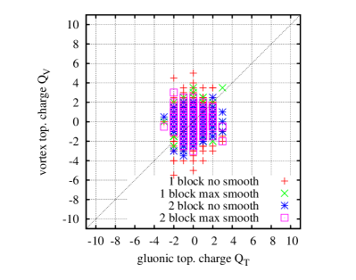
Figure 21: Scatter plot of the vortex vs. gluonic topological charge for original (full) $SU(2)$ and vortex smeared configurations. Vortex topological charge determination after a),b) one and c),d) two blocking steps and a),c) no and b),d) maximal smoothing. In e/f we show the combined results (a-d) for blocked flux distribution smeared configurations again.

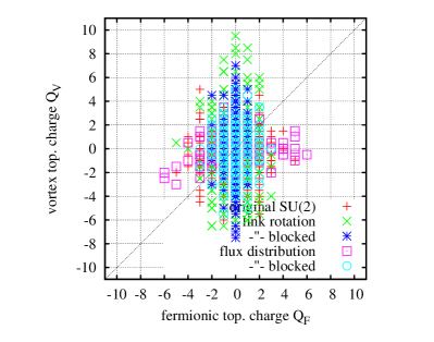
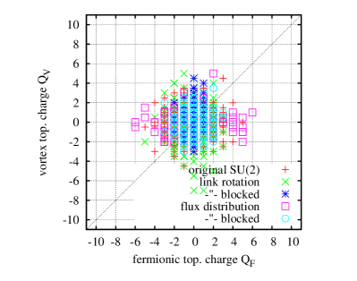
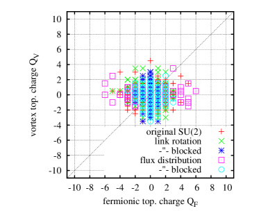
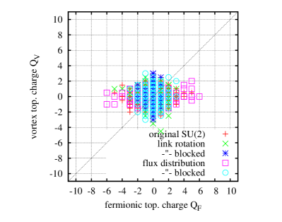
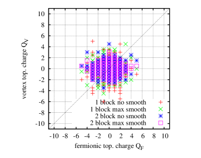
a) b) c) d) e) f)

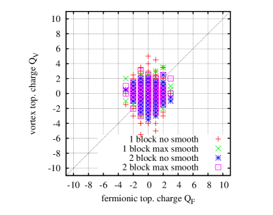
Figure 22: Scatter plot of the vortex vs. fermionic topological charge for original (full) $SU(2)$ and vortex smeared configurations. Vortex topological charge determination after a),b) one and c),d) two blocking steps and a),c) no and b),d) maximal smoothing. In e/f we show the combined results (a-d) for blocked flux distribution smeared configurations again.

In Fig. 23 we show the topological susceptibilities for original (full) $SU(2)$ and a) link rotation or b) flux distribution smeared configurations. The first thing we note is that for our original $SU(2)$ gauge ensemble, the topological susceptibilities from fermionic and gluonic topological charge definitions are not consistent, $\langle Q_{F}^{2}\rangle/V=(200$MeV$)^{4}$ and $\langle Q_{T}^{2}\rangle/V=(160$MeV$)^{4}$ (averaging cooling and smearing $Q_{T}$), presumably caused by our small original lattice volume of about $(1.2$fm$)^{4}$. It is very interesting, however, that the vortex topological susceptibility reproduces these values with one, respectively two blocking steps, averaging over the corresponding smoothing steps, see red dots/lines in Fig. 23. Next, we see that for the refined smeared configurations the gluonic and vortex topological charges (green dots and dashed lines) lead to much higher susceptibilities, caused by the artificial vortex fluctuations introduced during the refined smearing process giving many (extra) contributions to $\mathcal{F}_{\mu\nu}\tilde{\mathcal{F}}_{\mu\nu}$. This effect is larger for link rotation (Fig. 23a) compared to flux distribution smearing (Fig. 23b). After blocking, however,the original results are reproduced, shown in the lower plots in each case, i.e., compare red and blue dots/lines in Fig. 23c and d. The gluonic topological susceptibilities after cooling and (LOG) smearing (blue dashed lines) agree with the original values (red dashed lines) and vortex topological charge also matches the original averages (blue and red dots). Concerning fermionic topological susceptibility (solid lines), the refined link rotation smearing reproduces a value of $\langle Q_{F}^{2}\rangle/V=(180$MeV$)^{4}$; after smeared blocking, the value drops to $(95$MeV$)^{4}$, however. The vortex flux distribution smearing method gives a more reasonable result, perfectly consistent with gluonic and vortex topological susceptibilities. The refined version of flux distribution smearing gives a topological susceptibility from fermionic $Q_{F}$ of $(260$MeV$)^{4}$, which lies exactly between the gluonic values after cooling or LOG smearing for the refined flux distribution smeared configurations. After blocking this value drops to $(160$MeV$)^{4}$, consistent with gluonic topological charge susceptibilities from original (full) SU(2) and vortex flux smeared and blocked configurations. For our rather small original lattices of about $(1.2$fm$)^{4}$, a topological susceptibility of roughly $(160$MeV$)^{4}$ seems reasonable and we find that all definitions of topological charge agree on this value after appropriate smearing and blocking, as the lower plots at $a=0.6$fm show. The results confirm that vortices are indeed able to reproduce the topological susceptibility of full QCD, either via vortex topological charge or gluonic and fermionic definitions after vortex smearing.

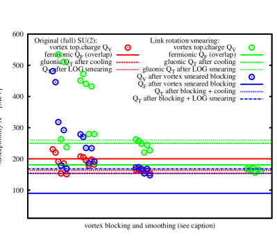
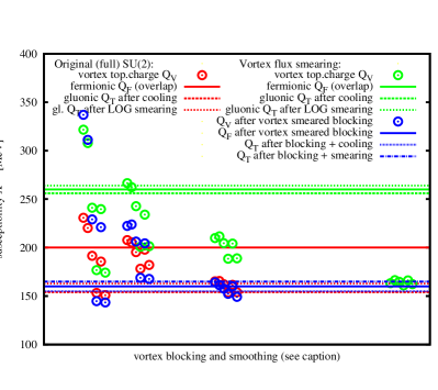
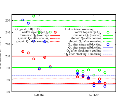
a) b) c) d)

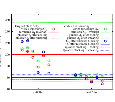
Figure 23: Topological susceptibility from fermionic $Q_{F}$, gluonic $Q_{T}$ and vortex topological charge $Q_{V}$ for original (full) $SU(2)$ (red) and refined a),c) link rotation (see Sec. II.4) or b),d) vortex flux distribution (see Sec. II.5) smeared (green) and blocked (blue, see Sec. II.6) configurations. In a) and b) we show all blocking and smearing steps for $Q_{V}$, i.e., we see four vertical groups of data points according to no, one, two and three blocking steps from left to right. Within these groups we plot the data points for zero to five smoothing steps from left to right again. In c) and d) we show 1-2 blocking steps for $8^{4}$ lattices, i.e., original and smeared blocked configurations, and 2-3 blocking steps for refined ($16^{4}$) lattices, resulting in lattice spacings $a\approx 0.3-0.6$fm respectively. We also zoom into the interesting susceptibility region and therefore miss a few data points from vortex topological charge $Q_{V}$ (green dots in a and c) and the blue line for topological susceptibility from fermionic $Q_{F}$ for blocked link rotation smearing (blue solid line) in c. Note that for original (full) $SU(2)$, the topological susceptibilities from fermionic (red solid line) and gluonic topological charge definitions (red dashed lines) are not consistent, $\langle Q_{F}^{2}\rangle/V=(200$MeV$)^{4}$ and $\langle Q_{T}^{2}\rangle/V\approx(160$MeV$)^{4}$ (averaging data from cooling and LOG smearing $Q_{T}$), presumably caused by our small original lattice volume of about $(1.2$fm$)^{4}$. Vortex topological charge $Q_{V}$ (red dots) reproduces the two values after one resp. two blocking steps in c) or d). Refined smeared configurations (green) show very high susceptibilities for gluonic and vortex topological charge, caused by artificial vortex fluctuations introduced in the refined smearing methods. Blocking removes these fluctuations and we observe good agreement between the different topological charge definitions on original and vortex smeared configurations, especially for the vortex flux distribution smearing - see d) at $a=0.6$fm (i.e., two blocking steps for $Q_{V}$).

III.4 Center Vortex and Dirac Eigenmode Correlations

We analyze the correlation of the overlap Dirac zero mode and first asqtad staggered Dirac eigenmode of the vortex smeared configurations to the original vortex structure. We use the correlator $C_{\lambda}(N_{\rm v})=\frac{\sum_{p_{i}}\sum_{x\in H}(V\rho_{\lambda}(x)-1)}{\sum_{p_{i}}\sum_{x\in H}1}$ Kovalenko:2005rz , where the sum is over sites $p_{i}$ on the dual lattice which belong to $N_{\rm v}$ plaquettes on the vortex surface (as identified from center projection), $\rho_{\lambda}(x)$ is the eigenmode density and $V$ is the lattice volume. At each such vortex site on the dual lattice there is a second sum ($x\in H$) over sites in a hypercube on the original lattice surrounding $p_{i}$. This correlator gives the relative enhancement of the eigenmode density at the vortex surface. A similar quantity $C_{\lambda}(q_{\rm v})$ can be formulated for vortex topological charge density $q_{\rm v}$, with $p_{i}$ the sites on the dual lattice carrying vortex topological charge $q_{\rm v}$.

In Figs. 24 and 25 we display the data for $C_{\lambda}(N_{\rm v})$ resp. $C_{\lambda}(q_{\rm v})$ computed for overlap and staggered eigenmodes on the original (full), center projected $Z(2)$ and various smeared configurations. We see that for refined vortex smeared configurations the eigenmodes are strongly correlated to the vortex surface and topological charge. The anti-correlation of overlap eigenmodes for the $Z(2)$ (center projected) configurations is completely removed after refined smearing, however after smeared blocking we lose the correlation to the original vortex structure again. We tried to extend the second sum ($\sum_{x\in H}$ in $C_{\lambda}$) to next-to-nearest neighbors but then the signal is lost in the background noise, i.e., we practically sum over all sites where the correlator gives zero per definition. In the case of asqtad staggered eigenmodes we get good correlations for all cases. The refined smeared configurations show drastically enhanced correlations whereas blocked smeared results lie between original SU(2) and center projected $Z(2)$ correlations.

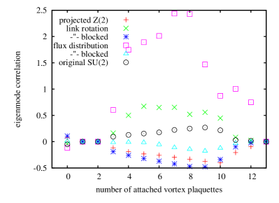
a) b)

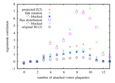
Figure 24: Vortex correlation of a) overlap and b) asqtad staggered eigenmodes for original (full) $SU(2)$, Maximal Center Gauge projected $Z(2)$ and vortex smeared configurations.

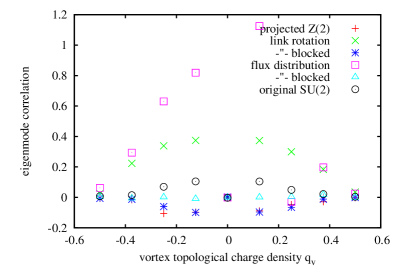
a) b)

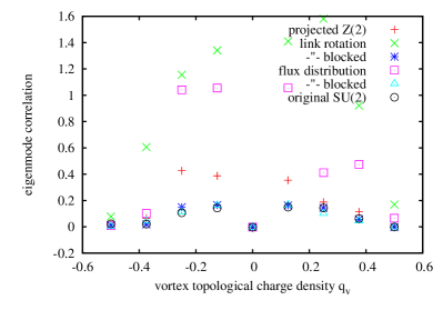
Figure 25: Correlation of vortex topological charge density with a) overlap zero mode and b) lowest asqtad staggered eigenmode densities for original (full) $SU(2)$, center projected $Z(2)$ and vortex smeared configurations.

III.5 Wilson Loops and Vortex Limited Wilson Loops

In Fig. 26 we show the standard and center projected Wilson loops of original $SU(2)$ vs. vortex smeared configurations. Plaquettes are systematically minimized during smearing, hence small smeared Wilson loops tend to be much closer to $\mathbbm{1}$. The $Z(2)$ Wilson loops, i.e., Wilson loops after MCG and center projection, for smeared blocked configurations however seem to reproduce the original $Z(2)$ Wilson loops.

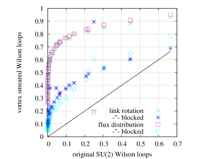
a) b)

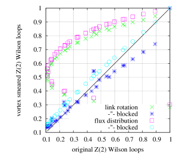
Figure 26: Scatter plot of a) $SU(2)$ and b) $Z(2)$ Wilson loops during smearing for original and various vortex smeared configurations.

In Fig. 27a we show the ratios of vortex limited Wilson loops, i.e., Wilson loop averages $W_{i}$ evaluated on subsets of loops with $i$ original vortex piercings. The results show that the vortex structure is preserved, only for large Wilson loops on blocked smeared lattices the signal becomes weak. Finally, in Fig. 27b we plot the Creutz ratios $\chi(R,R)$ which give for $R\rightarrow\infty$ the asymptotic string tension. We find that the vortex smeared configurations reproduce the original string tension, but not the Coulomb interaction for small $R$.

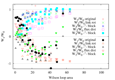
a) b)

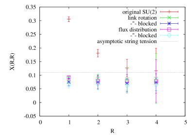
Figure 27: a) Vortex limited Wilson loops and b) Creutz ratios of original (full) $SU(2)$ and various vortex smeared configurations.

IV Vortex Smearing and Classical Configurations

Finally, we also tested the vortex smearing method on classical vortex configurations, namely planar and spherical vortices. The figures give an overview of the effects during vortex smearing and nicely illustrate the individual steps.

IV.1 Planar Vortex Pairs

Plane vortices are constructed as presented in Jordan:2007ff ; Hollwieser:2011uj . Due to the periodic boundary conditions of our lattice the vortex planes always appear in pairs and we analyze two vortex pairs in perpendicular directions, i.e., $xy$- and $zt$-vortices. They intersect at four space-time points, which contribute to the topological charge with contributions $Q=\pm 1/2$ depending on the orientation of the intersecting vortex sheets. After vortex smearing we may get total topological charge $Q=-2,-1,0,1$ or $2$, however the smearing routine seems to prefer the cases of even $Q$ ($-2,0$ and $2$). In fact, $Q=|1|$ requires orientation changes of single vortex sheets, which would introduce magnetic monopoles and therefore additional gauge singularities which seem to be suppressed by the minimizing of the plaquettes.

Fig. 28 shows the vortex configuration on the initial $8^{4}$ lattice, after refinement, vortex smearing and smoothing on the refined $16^{4}$ lattice. As stated above, refinement gives exactly the same vortex configuration on a finer lattice, whereas the smearing routine seems to distort the plane vortex sheets. However, after smoothing the smeared vortex surface as defined in Bertle:1999tw , all distortions are removed in the case of plane vortex sheets. After blocking even the unsmoothed smeared vortex configuration reveals the initial configuration.

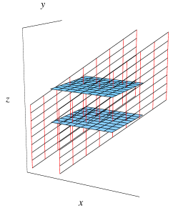
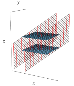
a) b) c)

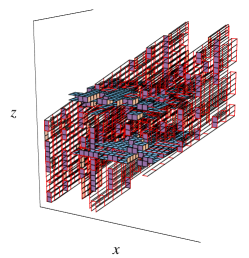
Figure 28: Two orthogonal pairs of planar vortices a) on a $8^{4}$ lattice and after b) refinement and c) vortex smearing on $16^{4}$ lattices. For a more detailed view of the configuration in c) see Fig. 29. Smoothing c) gives b) and blocking c) (or b) gives a). We plot the dual vortex plaquettes, which actually represent the closed vortex surfaces.

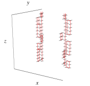
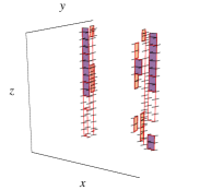
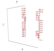
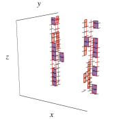
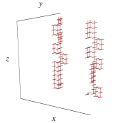
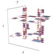
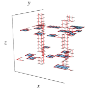
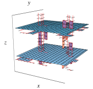
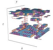
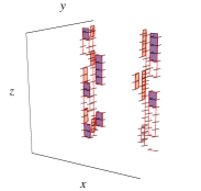
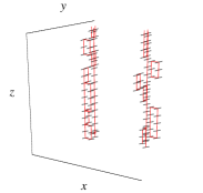
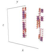
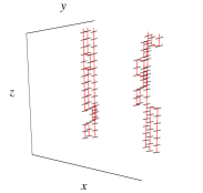
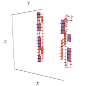
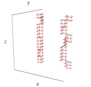
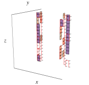
Figure 29: Dual vortex plaquettes of two orthogonal pairs of planar vortices after vortex smearing on $16^{4}$ lattices from Fig. 28c). From left to right and top to bottom we plot the single time slices (t=1-16).

IV.2 Spherical Vortex

The spherical vortex was introduced in Jordan:2007ff and analyzed in more detail in Hollwieser:2010mj and Schweigler:2012ae . The thin (Z(2)) vortex surface is given by a three dimensional sphere, which we put in a single time slice. In the thick vortex representation we can define an orientable and a non-orientable spherical vortex, which are characterized by topological charge $Q=0$ and $Q=\pm 1$. The latter shows a hedgehog like structure of gauge links at the vortex surface, the 3-sphere, defining a map $S^{3}\to SU(2)$ which is characterized by a winding number which yields the non-zero topological charge $Q$. Smearing the thin vortex, without any information on orientation, is very unlikely to reproduce the hedgehog-like structure and therefore always gives the $Q=0$ case. The vortex structure itself however, even though distorted during the smearing procedure, is nicely recovered during smoothing and perfectly after blocking, see Fig. 30.

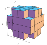
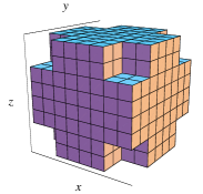
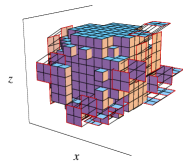
a) b) c) d)

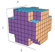
Figure 30: The spherical vortex a) on a $8^{4}$ lattice and after b) refinement, c) vortex smearing and d) smoothing on $16^{4}$ lattices. Blocking the configuration in c) (or b or d) gives a). We plot the dual vortex plaquettes, representing the closed vortex surface.

V Conclusions

We presented a method to smear $Z(2)$ vortex configurations such as to recover thick vortices with $SU(2)$ Yang-Mills information. The main goal was to remove the eigenvalue gap observed for overlap fermions in center projected $Z(2)$ vortex configurations. In order to maintain the original vortex structure we have to put the $Z(2)$ configurations on finer lattices, where we implemented two different smearing methods. On the refined lattice we can distribute the center vortex flux of the (dual) vortex plaquettes straightforwardly onto the refined plaquettes making up the original vortex plaquette. On the other hand, we can smear in terms of link variables, applying a smooth link profile, i.e., a ”slow” rotation of the links within several lattice spacings instead of the sudden jump from $+\mathbbm{1}$ to $-\mathbbm{1}$ or the other way around, which characterizes the vortex surface. Both approaches thicken the vortices in the sense that the center flux is not restricted to a singular surface but spread out over a few lattice spacings. The refinement procedure applied to the $Z(2)$ configurations, although preserving the exact vortex structure, causes new obstacles for lattice fermions, especially for the staggered Dirac operator, which are supposedly related to discretization effects. For the staggered operator these seem to be caused by its special implementation with even/odd lattices and are hard to overcome with smearing methods. For the overlap operator however, we can optimize our smearing routines to close the eigenvalue gap and reproduce a finite number of actual zero modes. Besides the refined smearing methods, we also discuss a method to block the smeared lattice back to its original size. With the various methods we can also reproduce topological properties of the original gauge fields; on blocked vortex smeared lattices the different definitions of topological charge, i.e., fermionic, gluonic and vortex topological charge, result in comparable susceptibilities. However, one-to-one correlations of topological aspects for individual configurations are not observed. The reason was discussed in detail above and can be summarized in a simple manner. Gluonic topological charge definitions are usually applied after cooling or smearing, both transforming Monte Carlo configurations into smooth gauge fields without center vortex excitations. Thin center vortex gauge fields, i.e., $Z(2)$ configurations, on the other hand lack any information of the orientation of thick center vortices, which is crucial for topological charge determination. During vortex smearing or vortex topological charge determination we apply random orientations to the vortex sheets and cannot expect to reproduce the original topological charge. However, earlier results and the analysis here show that vortex gauge fields reproduce the net topological charge and susceptibility via vortex topological charge definition and via fermionic or gluonic definitions after the introduced vortex smearing methods. The vortex smeared configurations, besides preserving the original vortex structure, also reproduce the asymptotic string tension of the original gauge field ensemble, which is the basis of the confinement mechanism by center vortices. It should be stressed that our method is not intended to reproduce full Yang-Mills dynamics on arbitrarily short length scales, but rather to encode the infrared dynamics consistently in fields which only vary appreciably over lengths commensurate with an infrared effective picture. This consistency is, strictly speaking, not manifest as long as one remains in a thin P-vortex framework. In the process, properties are seen to be recovered which are not accessible using pure $Z(2)$ configurations. In accordance with this, it should be remarked that, although we primarily have not analyzed the scaling behavior of our smeared ensembles due to the considerable numerical effort associated with the refined lattices, we do not envisage reproducing a particular scaling law with the smeared degrees of freedom. Rather, the center vortex picture as an infrared effective model has a fixed scale given by the vortex thickness, which acts as an ultraviolet cutoff and has a direct relation to $\Lambda_{QCD}$. Starting from (thin) $Z(2)$ vortices our smearing method tries to regain the finite vortex thickness, which then sets the initial scale and allows us to extract observables within these infrared effective degrees of freedom. Going forward in that sense, the plan is to use the developed tools to analyze topological and fermionic properties of the $SU(2)$ effective center vortex model Engelhardt:1999wr . Further, the methods shall be advanced to the $SU(3)$ gauge group and applied to the corresponding vortex model Engelhardt:2003wm .

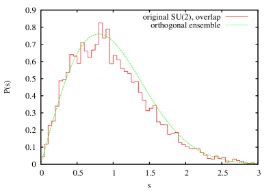
a) b) c) d) e) f)

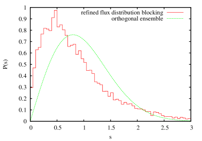
Figure 31: ”Unfolded” level spacing of overlap eigenvalues in the fundamental representation of SU(2) (orthogonal ensemble) for a) all, b) original and c-d) smeared configs: c) link rotation smearing, d) flux distribution smearing and their blocked versions in e) and f), respectively.

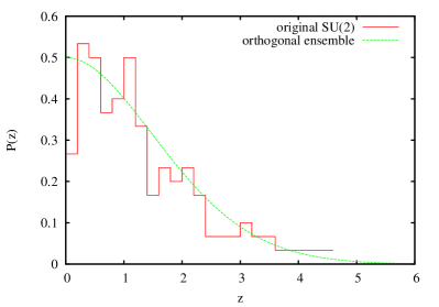
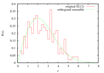
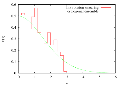
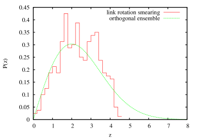
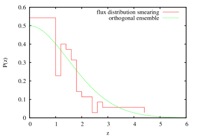
a) b) c) d) e) f)

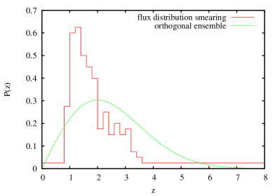
Figure 32: Distribution of lowest overlap eigenvalues in the fundamental representation of SU(2) (orthogonal ensemble) for a-b) original, c-d) link rotation and e-f) flux distribution smearing in topological sectors $\nu=0$ (left) and $\nu=1$ (right).

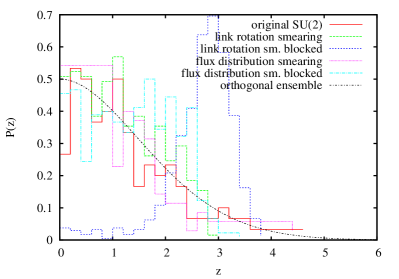
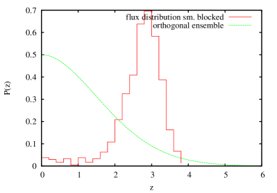
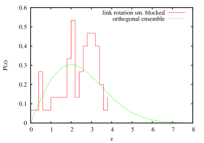
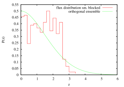
a) b) c) d) e) f)

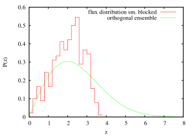
Figure 33: Distribution of lowest overlap eigenvalues in the fundamental representation of SU(2) (orthogonal ensemble) for a-b) combined configurations, c-d) link rotation and e-f) flux distribution smeared blocking in topological sectors $\nu=0$ (left) and $\nu=1$ (right).

Appendix B: Staggered Fermion Mode Distributions

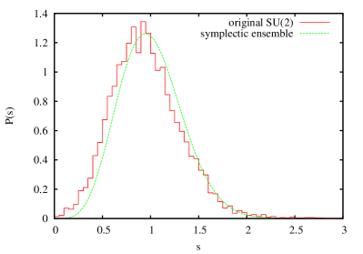
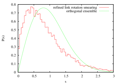
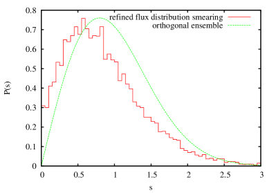
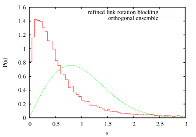
a) b) c) d) e) f)

Figure 34: ”Unfolded” level spacing of staggered eigenvalues in the fundamental representation of SU(2) (symplectic ensemble) for a) all, b) original and c-f) smeared configurations: c) link rotation smearing, d) flux distribution smearing and their blocked versions in e) and f), respectively.

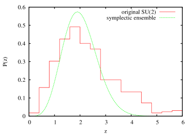
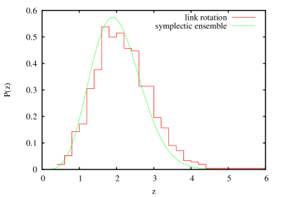
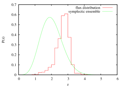
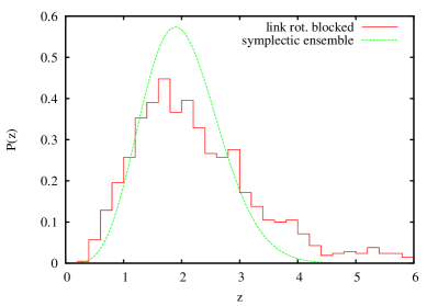
a) b) c) d) e) f)

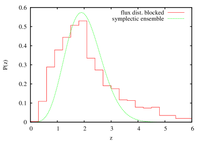
Figure 35: Distribution of lowest staggered eigenvalues in the fundamental representation of SU(2) (symplectic ensemble) for a) all, b) original and c-f) smeared configurations: c) link rotation and d) flux distribution smearing and their blocked versions in e) and f), respectively.

References

- (1) G. ’t Hooft, “On the phase transition towards permanent quark confinement,” Nucl. Phys. B138 (1978) 1.
- (2) P. Vinciarelli, “Fluxon solutions in nonabelian gauge models,” Phys. Lett. B78 (1978) 485–488.
- (3) T. Yoneya, “Z(n) topological excitations in yang-mills theories: Duality and confinement,” Nucl. Phys. B144 (1978) 195.
- (4) J. M. Cornwall, “Quark confinement and Vortices in massive gauge invariant QCD,” Nucl. Phys. B157 (1979) 392.
- (5) H. B. Nielsen and P. Olesen, “A Quantum Liquid Model for the QCD Vacuum: Gauge and Rotational Invariance of Domained and Quantized Homogeneous Color Fields,” Nucl. Phys. B160 (1979) 380.
- (6) We use direct maximal center gauge, which is equivalent to Landau gauge in the adjoint representation, and which maximizes the squared trace of link variables.
- (7) L. Del Debbio, M. Faber, J. Greensite, and Š. Olejník, “Center dominance and Z(2) vortices in SU(2) lattice gauge theory,” Phys. Rev. D 55 (1997) 2298–2306, arXiv:9610005 [hep-lat].
- (8) K. Langfeld, H. Reinhardt, and O. Tennert, “Confinement and scaling of the vortex vacuum of SU(2) lattice gauge theory,” Phys. Lett. B419 (1998) 317–321, arXiv:9710068 [hep-lat].
- (9) L. Del Debbio, and M. Faber, and J. Greensite, and Š. Olejník, “Center dominance, center vortices, and confinement,” arXiv:9708023 [hep-lat].
- (10) T. G. Kovacs and E. T. Tomboulis, “Vortices and confinement at weak coupling,” Phys. Rev. D 57 (1998) 4054–4062, arXiv:9711009 [hep-lat].
- (11) M. Engelhardt and H. Reinhardt, “Center vortex model for the infrared sector of Yang-Mills theory: Confinement and deconfinement,” Nucl.Phys. B585 (2000) 591–613, arXiv:hep-lat/9912003 [hep-lat].
- (12) M. Engelhardt, M. Quandt, and H. Reinhardt, “Center vortex model for the infrared sector of SU(3) Yang-Mills theory: Confinement and deconfinement,” Nucl.Phys. B685 (2004) 227–248, arXiv:0311029 [hep-lat].
- (13) R. Höllwieser, D. Altarawneh, and M. Engelhardt, “Random center vortex lines in continuous 3D space-time,” AIP Conf. Proc. ConfinementXI (2014) to appear, arXiv:1411.7089 [hep-lat].
- (14) D. Altarawneh, R. Höllwieser and M. Engelhardt, “Confining Bond Rearrangement in Random Center Vortex Models,” (submitted to JHEP) (2015) , arXiv:1508.07596 [hep-lat].
- (15) R. Höllwieser and D. Altarawneh, “Center Vortices, Area Law and the Catenary Solution,” (submitted to PRD) (2015) , arXiv:1509.00145 [hep-lat].
- (16) R. Bertle, M. Engelhardt, and M. Faber, “Topological susceptibility of Yang-Mills center projection vortices,” Phys. Rev. D 64 (2001) 074504, arXiv:0104004 [hep-lat].
- (17) M. Engelhardt, “Center vortex model for the infrared sector of Yang-Mills theory: Topological susceptibility,” Nucl.Phys. B585 (2000) 614, arXiv:0004013 [hep-lat].
- (18) M. Engelhardt, “Center vortex model for the infrared sector of SU(3) Yang-Mills theory: Topological susceptibility,” Phys. Rev. D 83 (2011) 025015, arXiv:1008.4953 [hep-lat].
- (19) R. Höllwieser, M. Faber, U.M. Heller, “Lattice Index Theorem and Fractional Topological Charge,” arXiv:1005.1015 [hep-lat].
- (20) R. Höllwieser, M. Faber, U.M. Heller, “Intersections of thick Center Vortices, Dirac Eigenmodes and Fractional Topological Charge in SU(2) Lattice Gauge Theory,” JHEP 1106 (2011) 052, arXiv:1103.2669 [hep-lat].
- (21) T. Schweigler, R. Höllwieser, M. Faber and U.M. Heller, “Colorful SU(2) center vortices in the continuum and on the lattice,” Phys.Rev. D87 no. 5, (2013) 054504, arXiv:1212.3737 [hep-lat].
- (22) R. Höllwieser, M. Faber, U.M. Heller, “Critical analysis of topological charge determination in the background of center vortices in SU(2) lattice gauge theory,” Phys. Rev. D 86 (2012) 014513, arXiv:1202.0929 [hep-lat].
- (23) R. Höllwieser and M. Engelhardt, “Smearing Center Vortices,” PoS LAT2014 (2014) 356, arXiv:1411.7097 [hep-lat].
- (24) P. de Forcrand and M. D’Elia, “On the relevance of center vortices to QCD,” Phys. Rev. Lett. 82 (1999) 4582–4585, arXiv:hep-lat/9901020 [hep-lat].
- (25) C. Alexandrou, P. de Forcrand, and M. D’Elia, “The role of center vortices in QCD,” Nucl. Phys. A663 (2000) 1031–1034, arXiv:hep-lat/9909005 [hep-lat].
- (26) M. Engelhardt and H. Reinhardt, “Center projection vortices in continuum Yang-Mills theory,” Nucl. Phys. B567 (2000) 249, arXiv:9907139 [hep-th].
- (27) M. Engelhardt, “Center vortex model for the infrared sector of Yang-Mills theory: Quenched Dirac spectrum and chiral condensate,” Nucl.Phys. B638 (2002) 81–110, arXiv:hep-lat/0204002 [hep-lat].
- (28) D. Leinweber, P. Bowman, U. Heller, D. Kusterer, K. Langfeld, et al., “Role of centre vortices in dynamical mass generation,” Nucl.Phys.Proc.Suppl. 161 (2006) 130–135.
- (29) V. Bornyakov et al., “Interrelation between monopoles, vortices, topological charge and chiral symmetry breaking: Analysis using overlap fermions for SU(2),” Phys. Rev. D 77 (2008) 074507, arXiv:0708.3335 [hep-lat].
- (30) R. Höllwieser, M. Faber, J. Greensite, U.M. Heller, and Š. Olejník, “Center Vortices and the Dirac Spectrum,” Phys. Rev. D 78 (2008) 054508, arXiv:0805.1846 [hep-lat].
- (31) R. Höllwieser, Center vortices and chiral symmetry breaking. PhD thesis, Vienna, Tech. U., Atominst., 2009-01-11. http://katalog.ub.tuwien.ac.at/AC05039934.
- (32) P. O. Bowman, K. Langfeld, D. B. Leinweber, A. Sternbeck, L. von Smekal, et al., “Role of center vortices in chiral symmetry breaking in SU(3) gauge theory,” Phys.Rev. D84 (2011) 034501, arXiv:1010.4624 [hep-lat].
- (33) R. Höllwieser, T. Schweigler, M. Faber and U.M. Heller, “Center Vortices and Chiral Symmetry Breaking in SU(2) Lattice Gauge Theory,” Phys.Rev. D88 (2013) 114505, arXiv:1304.1277 [hep-lat].
- (34) R. Höllwieser, M. Faber, Th. Schweigler, and U.M. Heller, “Chiral Symmetry Breaking from Center Vortices,” PoS LAT2013 (2014) 505, arXiv:1410.2333 [hep-lat].
- (35) D. Trewartha, W. Kamleh, and D. Leinweber, “Centre Vortex Effects on the Overlap Quark Propagator,” PoS LATTICE2014 (2014) 357, arXiv:1411.0766 [hep-lat].
- (36) D. Trewartha, W. Kamleh, and D. Leinweber, “Evidence that centre vortices underpin dynamical chiral symmetry breaking in SU(3) gauge theory,” Phys. Lett. B747 (2015) 373–377, arXiv:1502.06753 [hep-lat].
- (37) J. Greensite and R. Höllwieser, “Double-winding Wilson loops and monopole confinement mechanisms,” Phys. Rev. D91 no. 5, (2015) 054509, arXiv:1411.5091 [hep-lat].
- (38) We also want to mention a similar attempt to smear vortices in Bruckmann:2003yd , although for an explicit example of a vortex configuration and with a different goal, i.e., to understand topological charge contributions from vortex writhe and intersections. In the present investigation we want to develop a smearing method for random vortex configurations.
- (39) F. Bruckmann and M. Engelhardt, “Writhe of center vortices and topological charge: An Explicit example,” Phys. Rev. D 68 (2003) 105011, arXiv:0307219 [hep-th].
- (40) M. Lüscher, “Topology of Lattice Gauge Fields,” Commun.Math.Phys. 85 (1982) 39.
- (41) To each cell on the original lattice corresponds a cell of the dual lattice, where is the dimension of the lattice. The dual lattice is shifted with respect to the original lattice half a lattice spacing in each direction. In four dimensions, there is a one-to-one correspondence between original and dual plaquettes, i.e., -plaquettes correspond to -plaquettes etc. and corresponding plaquettes share the same center point.
- (42) M. Falcioni, M. Paciello, G. Parisi, and B. Taglienti, “AGAIN ON SU(3) GLUEBALL MASS,” Nucl.Phys. B251 (1985) 624–632.
- (43) M. Teper, “An Improved Method for Lattice Glueball Calculations,” Phys.Lett. B183 (1987) 345.
- (44) APE Collaboration Collaboration, M. Albanese et al., “Glueball Masses and String Tension in Lattice QCD,” Phys.Lett. B192 (1987) 163–169.
- (45) C. Morningstar and M. J. Peardon, “Analytic smearing of SU(3) link variables in lattice QCD,” Phys.Rev. D69 (2004) 054501, arXiv:hep-lat/0311018 [hep-lat].
- (46) A. Hasenfratz, R. Hoffmann, and S. Schaefer, “Hypercubic smeared links for dynamical fermions,” JHEP 0705 (2007) 029, arXiv:hep-lat/0702028 [hep-lat].
- (47) S. Durr, “Logarithmic link smearing for full QCD,” Comput.Phys.Commun. 180 (2009) 1338–1357, arXiv:0709.4110 [hep-lat].
- (48) R. Bertle, M. Faber, J. Greensite, and Š. Olejník, “The structure of projected center vortices in lattice gauge theory,” JHEP 03 (1999) 019, arXiv:9903023 [hep-lat].
- (49) The MIMD Lattice Computation (MILC) Collaboration: http://www.physics.utah.edu/ detar/milc.
- (50) R. Narayanan and H. Neuberger, “A construction of lattice chiral gauge theories,” Nucl. Phys. B443 (1995) 305–385, arXiv:9411108 [hep-th].
- (51) H. Neuberger, “Exactly massless quarks on the lattice,” Phys. Lett. B417 (1998) 141–144, arXiv:9707022 [hep-lat].
- (52) H. Leutwyler and A. Smilga, “Spectrum of Dirac operator and role of winding number in QCD,” Phys. Rev. D 46 (1992) 5607–5632.
- (53) M. Berbenni-Bitsch, S. Meyer, A. Schafer, J. Verbaarschot, and T. Wettig, “Microscopic universality in the spectrum of the lattice Dirac operator,” Phys.Rev.Lett. 80 (1998) 1146–1149, arXiv:hep-lat/9704018 [hep-lat].
- (54) R. G. Edwards, U. M. Heller, J. E. Kiskis, and R. Narayanan, “Quark spectra, topology and random matrix theory,” Phys.Rev.Lett. 82 (1999) 4188–4191, arXiv:hep-th/9902117 [hep-th].
- (55) J. Verbaarschot and T. Wettig, “Random matrix theory and chiral symmetry in QCD,” Ann.Rev.Nucl.Part.Sci. 50 (2000) 343–410, arXiv:hep-ph/0003017 [hep-ph].
- (56) A. M. Halasz and J. Verbaarschot, “Universal fluctuations in spectra of the lattice Dirac operator,” Phys.Rev.Lett. 74 (1995) 3920–3923, arXiv:hep-lat/9501025 [hep-lat].
- (57) P. Forrester, “The spectrum edge of random matrix ensembles,” Nucl. Phys. B402 (1993) 709–728.
- (58) T. Nagao and P. Forrester, “Asymptotic correlations at the spectrum edge of random matrices,” Nucl.Phys. B435 (1995) 401–420.
- (59) T. Nagao and P. Forrester, “The smallest eigenvalue distribution at the spectrum edge of random matrices,” Nucl.Phys. B509 (1998) 561–598.
- (60) P. Di Vecchia, K. Fabricius, G. C. Rossi, and G. Veneziano, “Preliminary Evidence for U(1)-A Breaking in QCD from Lattice Calculations,” Nucl. Phys. B192 (1981) 392.
- (61) P. Di Vecchia, K. Fabricius, G. C. Rossi, and G. Veneziano, “Numerical checks of the lattice definition independence of topological charge fluctuations,” Phys. Lett. B108 (1982) 323.
- (62) M. F. Atiyah and I. M. Singer, “The Index of elliptic operators. 5,” Annals Math. 93 (1971) 139–149.
- (63) L. Del Debbio, M. Faber, J. Giedt, J. Greensite, and Š. Olejník, “Detection of center vortices in the lattice Yang-Mills vacuum,” Phys.Rev. D58 (1998) 094501, arXiv:hep-lat/9801027 [hep-lat].
- (64) M. Engelhardt, K. Langfeld, H. Reinhardt, and O. Tennert, “Interaction of confining vortices in SU(2) lattice gauge theory,” Phys.Lett. B431 (1998) 141–146, arXiv:hep-lat/9801030 [hep-lat].
- (65) A. V. Kovalenko, S. M. Morozov, M. I. Polikarpov, and V. I. Zakharov, “On topological properties of vacuum defects in lattice yang-mills theories,” Phys. Lett. B648 (2007) 383–387, arXiv:0512036 [hep-lat].
- (66) G. Jordan, R. Höllwieser, M. Faber, U.M. Heller, “Tests of the lattice index theorem,” Phys. Rev. D 77 (2008) 014515, arXiv:0710.5445 [hep-lat].