Coupled Oscillator Model for Nonlinear Gravitational Perturbations

Abstract

Motivated by the gravity/fluid correspondence, we introduce a new method for characterizing nonlinear gravitational interactions. Namely we map the nonlinear perturbative form of the Einstein equation to the equations of motion of a collection of nonlinearly-coupled harmonic oscillators. These oscillators correspond to the quasinormal or normal modes of the background spacetime. We demonstrate the mechanics and the utility of this formalism within the context of perturbed asymptotically anti-de Sitter black brane spacetimes. We confirm in this case that the boundary fluid dynamics are equivalent to those of the hydrodynamic quasinormal modes of the bulk spacetime. We expect this formalism to remain valid in more general spacetimes, including those without a fluid dual. In other words, although borne out of the gravity/fluid correspondence, the formalism is fully independent and it has a much wider range of applicability. In particular, as this formalism inspires an especially transparent physical intuition, we expect its introduction to simplify the often highly technical analytical exploration of nonlinear gravitational dynamics.

I Introduction

Can spacetimes become turbulent? Direct numerical simulations of large asymptotically anti–de Sitter (AdS) black holes Adams et al. (2014) and their holographically dual fluids Carrasco et al. (2012); Green et al. (2014) have provided convincing evidence that this is the case. This phenomenon, perhaps counterintuitive at first glance, can be understood through the gravity/fluid correspondence Baier et al. (2008); Bhattacharyya et al. (2008a); Van Raamsdonk (2008). This correspondence links the behavior of long-wavelength perturbations of black holes in AdS to viscous relativistic hydrodynamics, and its regime of applicability can include cases of high Reynolds number on the fluid side. Spacetime turbulence then follows from turbulence in the dual fluid Van Raamsdonk (2008); Carrasco et al. (2012). On the gravity side, a high Reynolds number corresponds to dissipation of gravitational perturbations that is weak when compared with nonlinear interactions. It is therefore not surprising that it arises in the vicinity of asymptotically AdS black holes, which can have relatively long lived quasinormal modes.

The observation of gravitational turbulence in AdS motivates a further question: Can one analyze this striking nonlinear behavior directly in general relativity without relying on the existence of a holographic dual? That is, rather than borrowing from the dual hydrodynamic description—and any restricted regime of applicability—can one establish a bona-fide description of turbulence as a perturbative solution of the Einstein equation? Recall that turbulence is a nonlinear phenomenon characterized, in particular, by cascades of energy (and sometimes enstrophy) between wave numbers. It is therefore delicate to fully capture this behavior within ordinary perturbation theory without carrying it out to sufficiently high orders and performing a suitable resummation Green et al. (2014). In order to take into account the essential gravitational self-interactions of perturbations that are present in the Einstein equation we will require a more general perturbative framework.

In this work we introduce a nonlinear coupled-oscillator model to describe the interaction of quasinormal or normal modes of a background spacetime, in particular their mode-mode couplings. This proposal is a natural generalization of our earlier study of nonlinear scalar wave generation around rapidly-spinning asymptotically flat black holes Yang et al. (2015), where the back-reaction on the driving mode was neglected (we account for it properly in this paper). This previous model illustrated that the onset of turbulence in gravity does not require the spacetime to be asymptotically anti–de Sitter. In the nonlinear oscillator model presented here, the coupling between modes is accounted for explicitly and in real time as opposed to implicitly through a recursive scheme. Therefore the equations of motion provide solutions that are valid over longer time scales.

Within this model, nonlinear gravitational perturbations are described by excitations of modes (quasinormal or normal). For a given background spacetime, the collection of modes is parametrized by a particular set of frequencies, damping rates, and, at the nonlinear level, mode coupling coefficients. Through these parameters, we can quantitatively compare and contrast signatures of nonlinear gravitational perturbations in different backgrounds, in the same way that frequencies and damping rates alone characterize linear perturbations. In this way we can gain a better understanding of nonlinear interactions and associated phenomena (such as turbulence) in general relativity. The route taken when constructing this formalism essentially offers a new perspective on how to deal with nonlinear metric perturbations that is conducive to intuition building. This compares favorably with more traditional methods, where one has to contend with difficult technical details that often mask the underlying physics.

To provide a concrete example, we will apply our methods to study nonlinear perturbations of an asymptotically AdS black brane. The gravity/fluid correspondence applies in this case and the resulting coupled-oscillator system may be compared against the dual fluid. We find that our equations are consistent with the relativistic hydrodynamic equations provided by the duality. Although the agreement is expected, our derivation provides an explicit demonstration and a natural physical interpretation of the observed phenomena in terms of quasinormal modes. We emphasize that the derivations in the gravity and fluid sides are independent of each other, and so the treatment for gravitational perturbations does not depend on the existence of a dual fluid and can be applied to more general spacetimes.

In the interest of caution, we recall that quasinormal modes do not form a basis for generic metric perturbations (see Warnick (2013) for a recent discussion). For instance, consider linear perturbations of the (asymptotically flat) Kerr spacetime as an example (see also discussions in Sec. II). The signal sourced by some matter distribution comprises quasinormal modes, the late-time “tail” term, as well as a prompt piece that travels along the light cone. In this sense, our formalism is approximate as we consider only the quasinormal mode contributions. However, in many cases, such as the ringdown stage of binary black hole mergers or when considering long wavelength perturbations of an asymptotically AdS black brane, it is sufficient to track only the quasinormal modes, as they are the dominant part of the signal (see, e.g., Barranco et al. (2014), for a related discussion). In more general scenarios, we can always check the validity of our approximation by estimating the magnitudes of the other contributions.

This paper is organized as follows. In Sec. II, we introduce the general formalism of the nonlinear coupled-oscillator model, and compare it with traditional methods for handling nonlinear gravitational perturbations. In Sec. III, we briefly review the asymptotically AdS black brane spacetime and the gravity/fluid correspondence, and we analyze the boundary fluid in the mode-expansion picture. In Sec. IV, we apply the general formalism to the specific case of the asymptotically AdS black brane. We conclude in Sec. V. The gravitational constant $G$ and the speed of light $c$ are both set to one, unless otherwise specified. Appendices are provided to elaborate on certain details.

II General Formalism

In this section, we begin by reviewing the traditional approach to solving the Einstein equation using ordinary perturbation theory and assuming a series expansion in the perturbation amplitude. This method might not lend itself to easily capturing relevant phenomena like turbulence. In the case where the linearized dynamics take the form of independently evolving normal or quasinormal modes (in the absence or presence of dissipation, respectively), we then show how the nonlinear Einstein equation can be represented as a set of coupled oscillator equations, which is analogous to treatments of the Navier-Stokes equation in fluid dynamics, and is indeed capable of cleanly capturing turbulence. For simplicity, we restrict our discussion to vacuum spacetimes, but it is straightforward to generalize the analysis to spacetimes with a cosmological constant.

II.1 Ordinary perturbation theory

Given any metric $g_{\mu\nu}$, one can split it into the sum of a “background” metric and a “perturbation”,

$$g_{\mu\nu}=g^{\rm B}_{\mu\nu}+h_{\mu\nu}\,.$$ (1)

Without invoking any approximation, the vacuum Einstein equation may then be written as

$$R_{\mu\nu}(g^{\rm B})+R^{(1)}_{\mu\nu}(g^{\rm B},h)+R^{(2)}_{\mu\nu}(g^{\rm B},h)+\sum_{n=3}^{\infty}R^{(n)}_{\mu\nu}(g^{\rm B},h)=0\,,$$ (2)

where $R^{(n)}_{\mu\nu}(g^{\rm B},h)$ denotes the $n$th order Ricci tensor expanded about $g^{\rm B}_{\mu\nu}$. Explicitly, the linearized and second order terms are

$$R^{(1)}_{\mu\nu}\equiv\frac{1}{2}(-h_{|\mu\nu}-{h_{\mu\nu|\alpha}}^{\alpha}+{h_{\alpha\mu|\nu}}^{\alpha}+{h_{\alpha\nu|\mu}}^{\alpha})\,,$$ (3)

and

$$R^{(2)}_{\mu\nu}\equiv \frac{1}{4}\left[h^{\alpha\beta}{}_{|\nu}h_{\alpha\beta|\mu}+2\left(h_{\nu\alpha|\beta}-h_{\nu\beta|\alpha}\right)h_{\mu}{}^{\alpha|\beta}\right.$$

$$\left.+\left(h_{\alpha\mu|\nu}+h_{\alpha\nu|\mu}-h_{\mu\nu|\alpha}\right)\left(h_{\beta}{}^{\beta|\alpha}-2h^{\alpha\beta}{}_{|\beta}\right)\right.$$

$$\left.+2h^{\alpha\beta}\left(h_{\alpha\beta|\mu|\nu}+h_{\mu\nu|\alpha|\beta}-h_{\alpha\mu|\nu|\beta}-h_{\alpha\nu|\mu|\beta}\right)\right]\,.$$ (4)

In these expressions, covariant derivatives associated to the background metric $g^{\rm B}_{\mu\nu}$ are denoted by vertical lines. The background metric is also used to raise and lower indices.

As described in Wald (1984), ordinary perturbation theory assumes the existence of a one-parameter family of solutions $g_{\mu\nu}(\epsilon)$, where $g_{\mu\nu}(0)=g_{\mu\nu}^{\text{B}}$, and $h_{\mu\nu}$ depends differentiably on $\epsilon$. One can then Taylor expand the perturbation,

$$h_{\mu\nu}=\epsilon h^{(1)}_{\mu\nu}+\epsilon^{2}h^{(2)}_{\mu\nu}+\cdots.$$ (5)

Perturbative equations of motion of order $n$ follow by differentiating the Einstein equation (2) $n$ times with respect to $\epsilon$, and then setting $\epsilon=0$. At zeroth order we have simply

$$R_{\mu\nu}(g^{\text{B}})=0\,,$$ (6)

so that $g^{\text{B}}_{\mu\nu}$ is a vacuum solution itself.

At first order in $\epsilon$ we have the linearized Einstein equation,

$$R^{(1)}_{\mu\nu}(g^{\text{B}},h^{(1)})=0\,.$$ (7)

It is generally much easier to solve this equation (after making appropriate gauge choices and imposing boundary and initial conditions) than it is to solve the full Einstein equation. Then for sufficiently small $\epsilon$, $g_{\mu\nu}^{\text{B}}+\epsilon h_{\mu\nu}^{(1)}$ should be a good approximation to $g_{\mu\nu}(\epsilon)$.

This procedure may be continued to higher orders. For instance, at second order, we obtain

$$R^{(1)}_{\mu\nu}(g^{\text{B}},h^{(2)})=-R^{(2)}_{\mu\nu}(g^{\text{B}},h^{(1)})\,.$$ (8)

The second order perturbation is seen to evolve in the background spacetime $g^{\text{B}}_{\mu\nu}$, and it is sourced by the first order solution $h^{(1)}_{\mu\nu}$.

Generically, this approach reduces the nonlinear problem to a series of linear inhomogeneous problems of the form

$$R^{(1)}_{\mu\nu}(g^{\text{B}},h^{(n)})=S_{\mu\nu}^{(n)}(g^{\text{B}};h^{(1)},\ldots,h^{(n-1)})\,.$$ (9)

Thus, at each order, one solves a linear partial differential equation with a source, subject to appropriate boundary conditions and gauge choices. The left hand side of the equation at order $n$ consists always of the $n$th order perturbation $h^{(n)}_{\mu\nu}$ evolving linearly in the background spacetime $g^{\text{B}}_{\mu\nu}$. The source term $S_{\mu\nu}^{(n)}$ involves only already-solved lower order pieces $h_{\mu\nu}^{(m)}$ for $m<n$, so a higher order perturbation does not backreact on one of lower order. Moreover, since the $n$th order perturbation evolves in the zeroth order background metric—not the $(n-1)$th order metric—the efficient capture of parametric resonance type effects is precluded Green et al. (2014); Yang et al. (2015). (Of course, with enough intuition, it may be possible to identify this behavior through a suitable resummation of perturbations of sufficiently high order.) In following this program, the calculations are quite involved and the gauge choices at different orders are often subtle (see e.g., Bruni et al. (1997); Gleiser et al. (2000); Ioka and Nakano (2007); Brizuela et al. (2009)). In the specific context of extreme mass ratio binaries, recent examples of this program are given in Pound (2012); Gralla (2012).

II.2 Larger perturbations

After iterating the above procedure to any given order, the resulting perturbative metric should be a good approximation to $g_{ab}(\epsilon)$ for sufficiently small $\epsilon$. However, in certain situations one may be interested in studying systems with larger (but still small) values of $\epsilon$, where the Taylor expansion (5) either fails to converge or would require a large number of terms to obtain a good solution. Typically the perturbative solution would be valid for a short time, but for long times secular terms might dominate. Therefore, a more suitable scheme would be required. In, for example, the context of the Navier-Stokes equation, ordinary perturbation theory might be capable of capturing the initial onset of turbulence, but it would be ineffective in capturing fully developed turbulence (and likewise for gravitational turbulence Green et al. (2014); Yang et al. (2015)).

In order to characterize the nonlinear dynamics in general relativity in a more efficient and transparent manner, we present here an alternative way of obtaining approximate solutions that is better suited for exploring certain nonlinear phenomena such as wave interactions and turbulence. We assume as before that $g_{\mu\nu}^{\text{B}}$ satisfies the vacuum Einstein equation. But then, rather than Taylor expanding $h_{\mu\nu}$ as in (5), we consider the full metric perturbation $h_{\mu\nu}$, and we attempt to solve directly a truncated version of (2). In fact truncation at second order,

$$R^{(1)}_{\mu\nu}(g^{\text{B}},h)+R^{(2)}_{\mu\nu}(g^{\text{B}},h)=0\,,$$ (10)

captures the essential nonlinearities of interest to us here. We note that our formalism could straightforwardly be extended to higher orders, but for simplicity we restrict to second order nonlinearities here.

To summarize, instead of solving a tower of inhomogeneous linear equations (9) we solve a nonlinear equation, but we neglect the higher order nonlinearities. Instead of dealing with gauge issues at each order, we have only to impose the gauge condition once on $h_{\mu\nu}$. Of course, the truncation of the Ricci tensor is not a tensor itself so the equation (10) is not gauge invariant. But it should be sufficient to the order we are working ($O(h^{2})$). As we shall see, this approach readily captures the nonlinear mode coupling effects of interest to us.

In general it will be very difficult to solve (10), even neglecting the higher order nonlinearities as we have done. However, as we describe in the following subsection, in cases where the linear dynamics is dominated by the evolution of normal or quasinormal modes, (10) reduces to a system of nonlinearly coupled (and possibly damped) oscillators.

II.3 Expansion into modes

We now restrict consideration to background spacetimes whose linear perturbations are characterized (for some region of spacetime) by a set of modes (normal or quasinormal). In this case the first order metric perturbation may be written

$$h_{\mu\nu}^{(1)}(t,{\bf x})\sim\sum_{j}[q^{-}_{j}(t)\mathcal{Z}^{(j-)}_{\mu\nu}({\bf x})+q^{+}_{j}(t)\mathcal{Z}^{(j+)}_{\mu\nu}({\bf x})]\,,$$ (11)

with

$$q^{-}_{j}(t)=A_{j}e^{-i\omega_{j}t},\quad q^{+}_{j}(t)=B_{j}e^{i\omega^{*}_{j}t}\,.$$ (12)

The background spacetime is assumed to be stationary and the $t$ coordinate is the associated Killing parameter. Modes always occur in pairs with frequencies $\omega_{j}$ and $-\omega_{j}^{\ast}$, so we have organized the summation above along these lines, labeling each pair with a multi-index $j$ (denoting both the transverse harmonic and radial overtone). The associated spatial wave functions are denoted $\mathcal{Z}^{(j\pm)}_{\mu\nu}({\bf x})$. Finally, $q^{\pm}_{j}$ and $\{A_{j},B_{j}\}$ are the displacements and the amplitudes for modes $j\pm$, respectively. As $h_{\mu\nu}$ must be real at all time, we expect that $\{A_{j},B_{j}\}$ (as well as $\{\mathcal{Z}^{(j-)},\mathcal{Z}^{(j+)}\}$) are conjugate to each other.

The reason we organize our modes into pairs in (11) is to emphasize that all modes must be included in the nonlinear analysis; many linear analyses use symmetry arguments to only treat modes with $\Re(\omega)>0$ Berti et al. (2009). In the case of normal modes, the mode functions $\mathcal{Z}^{(j\pm)}_{\mu\nu}$ are degenerate and $\omega_{j}\in\mathbb{R}$, so we take $q_{j}=q^{-}_{j}+q^{+}_{j}=A_{j}e^{-i\omega_{j}t}+B_{j}e^{i\omega_{j}t}$. For quasinormal modes, the radial dependence of $\mathcal{Z}^{(j\pm)}_{\mu\nu}$, along with the dissipative boundary conditions at the horizon and/or infinity, fixes the time dependence of the mode uniquely. Any “degenerate” mode in this case must therefore have $\omega_{j}=-\omega_{j}^{\ast}$, so the frequency is purely imaginary, and the multi-index $j$ describes just a single mode. We analyze these cases separately from the non-degenerate case in the following sections.

Frequencies of quasinormal modes have nonzero positive imaginary part, which implies an exponential time decay as a result of energy dissipation. In addition, this complex frequency means that the mode functions generally blow up at spatial infinity and the horizon bifurcation surface. However, as physical observers effectively lie near null infinity, the quasinormal-mode signals they observe are finite and the modes are indeed physical perturbations of the spacetime. For such observers, the sum in (11) can become a good approximation over finite time intervals, although we remind the reader that quasinormal modes do not form a complete basis for generic metric perturbations. Additional contributions to the metric can arise at late times from waves being scattered by the background potential at large distances (the “tail” term), or at early times from a prompt signal (on the light cone) from the source (see, e.g., Leaver (1986); Kokkotas and Schmidt (1999); Berti et al. (2009); Casals et al. (2013)); we collect these into the “residual part”.

In this paper our focus is on mode-mode interactions and the associated coupling coefficients. We will therefore not consider the nonlinear interactions between the modes and the tail and prompt components of the metric perturbation. We caution, however, that such couplings need not always be small. While they are small for perturbations of AdS black branes in the hydrodynamic limit (which we analyze below), readers should keep in mind that they will lead to additional contributions to, e.g., Eq. (15) below. Furthermore, questions as to how quasinormal modes are excited by moving matter, or how to compute the excitation factors for these modes based on some arbitrary initial data are also beyond the scope of this work (see Leaver (1986); Hadar and Kol (2011); Zhang et al. (2013) and Appendix D).

With these observations in mind, following the discussion in Sec. II.2 we write the full metric perturbation as

$$h_{\mu\nu}(t,{\bf x}) = \sum_{j}[q^{-}_{j}(t)\mathcal{Z}^{(j-)}_{\mu\nu}({\bf x})+q^{+}_{j}(t)\mathcal{Z}^{(j+)}_{\mu\nu}({\bf x})]$$ (13)

$$\quad+\text{ residual part,}$$

but now generalizing the coefficients $A_{j}$ and $B_{j}$ to be functions of time,

$$q^{-}_{j}(t)=A_{j}(t)e^{-i\omega_{j}t},\quad q^{+}_{j}(t)=B_{j}(t)e^{i\omega^{*}_{j}t}\,.$$ (14)

Our task is to determine the nonlinear evolution of quasinormal modes; in other words, to evaluate the time dependence of $q^{\pm}_{j}$. Addressing this task is generally nontrivial as it requires the proper separation of the quasinormal modes from the residual part of the full metric perturbation. For Schwarzschild and Kerr spacetimes this is achievable by invoking the Green’s function technique (Appendix D), whereas the generalization of this approach to generic spacetimes remains an open problem. To present the coupled-oscillator model, we apply an alternative strategy of plugging (13) into the truncated Einstein equation (10) and projecting our the spatial dependencies, thereby obtaining mode evolution equations. This method is most accurate for dealing with normal-mode evolutions and cases where the residual parts are negligible (for example, see Sec. IV). In more general scenarios, we shall make several additional approximations (such as neglecting certain time derivatives, neglecting the residual part) to single out the ordinary differential equations for $q^{\pm}_{j}$. We also caution that since the set of modes generally does not form a complete basis, the resulting $h_{\mu\nu}$ is still only an approximate solution to the truncated Einstein equation. For simplicity, hereafter we shall not explicitly write down the residual part in the equations.

Upon substitution, the truncated Einstein equation (10) takes the form

$$\sum_{j}\sum_{s=\pm}\left[\rho_{j}^{s}({\bf x})\ddot{q}_{j}^{s}+\tau_{j}^{s}({\bf x})\dot{q}_{j}^{s}+\sigma_{j}^{s}({\bf x})q_{j}^{s}\right]$$ (15)

$$= O\left(q_{k}^{s^{\prime}}q_{l}^{s^{\prime\prime}},q_{k}^{s^{\prime}}\dot{q}_{l}^{s^{\prime\prime}},\dot{q}_{k}^{s^{\prime}}\dot{q}_{l}^{s^{\prime\prime}},q_{k}^{s^{\prime}}\ddot{q}_{l}^{s^{\prime\prime}}\right)\,.$$

Here $\rho_{j}^{s}$, $\tau_{j}^{s}$, and $\sigma_{j}^{s}$ are tensor functions of the spatial coordinates, and they depend on the background metric as well as the corresponding wave function of the quasinormal mode. The right hand side of the equation has a complicated $\bf x$-dependence that we have suppressed.

We would now like to project Eq. (15) onto individual modes to obtain equations for a set of nonlinearly coupled oscillators in the form of

$$a_{j}^{s}\ddot{q}_{j}^{s}+b_{j}^{s}\dot{q}_{j}^{s}+c_{j}^{s}q_{j}^{s}$$ (16)

$$= \hat{S}_{j}^{s}\left(q_{k}^{s^{\prime}}q_{l}^{s^{\prime\prime}},q_{k}^{s^{\prime}}\dot{q}_{l}^{s^{\prime\prime}},\dot{q}_{k}^{s^{\prime}}\dot{q}_{l}^{s^{\prime\prime}},q_{k}^{s^{\prime}}\ddot{q}_{l}^{s^{\prime\prime}}\right)\,,$$

for each $j$ and $s$. In order to do so we require a suitable set of projectors. If, along any of the dimensions transverse to the radial direction, the background metric possesses a suitable isometry group so that this part of the wave function is described by tensor harmonics (Fourier modes, tensor spherical harmonics, etc.) then it is easy to project out this part by using an inner product. The remaining part (generally including the radial direction) is however more problematic.

It is often the case that the equations can be written in the form of a standard eigenvalue problem, $\ddot{\Psi}=-A\Psi$. For normal modes, one can define an inner product $\langle\chi|\eta\rangle$ with respect to which $A$ is self-adjoint, and the modes are orthogonal. One can then use this inner product to define the projector. For dissipative systems with quasinormal modes, the eigenvalues are complex and $A$ cannot be self-adjoint. Another problem is that often $|\mathcal{Z}_{\mu\nu}^{(j\pm)}|\to\infty$ at the dissipative boundaries of the system. Nevertheless, it is still possible to define a suitable bilinear form, with respect to which $A$ is symmetric Leung et al. (1994, 1998, 1997); Yang et al. (2015); Zimmerman et al. (2014); Yang and Zhang (2014); Mark et al. (2015). This bilinear form involves an integral of $\chi\eta$ without any complex conjugation so symmetry of $A$ does not imply that the eigenvalues are real. Furthermore it is still necessary to appropriately regulate the integration to eliminate divergences. The bilinear form may be regarded as a “generalized” inner product, and be used as such. In particular, it may then be shown that $\langle\mathcal{Z}^{j\pm}|\mathcal{Z}^{k\pm}\rangle=0$ for $\omega_{j}\neq\omega_{k}$, and this orthogonality leads to a suitable projector.

In the general case (such as the coordinate system we use in Sec. IV) it is not necessarily possible to re-write the equation as a standard eigenvalue problem. Nevertheless, we can still define a generalized inner product and use it to project the equation onto modes. It may be that the modes are not orthogonal with respect to this inner product, in which case the projection of the left hand side of (10) contains contributions from additional modes beyond the desired projection mode. After performing projections onto all modes, it would then be necessary to diagonalize the system to obtain a set of equations of the form (16). This is possible by applying procedures described in Sec. II.3.1 to remove “unphysical modes” and reduce the order of the differential equations. At this point, it is worth noting that in principle any inner product which leaves this set of equations non-degenerate fits our purpose. However, in order to minimize the error from neglecting the residual part, it is good practice to adopt an inner-product suitable for eigenvalue perturbation analysis (see Sec. IV.2 for a concrete example of such an inner-product).

With the equations decoupled as in (16) with a suitable generalized inner product, we can now substitute in Eq. (14) for $q_{j}^{\pm}$. We obtain,

$$a_{j}^{-}\ddot{A}_{j}+\tilde{b}_{j}^{-}\dot{A}_{j} = S_{j}^{-}\left(A_{k},B_{l}\right),$$ (17)

$$a_{j}^{+}\ddot{B}_{j}+\tilde{b}_{j}^{+}\dot{B}_{j} = S_{j}^{+}\left(A_{k},B_{l}\right),$$ (18)

where $\tilde{b}_{j}^{-}\equiv b_{j}^{-}-2i\omega_{j}a_{j}^{-}$ and $\tilde{b}_{j}^{+}\equiv b_{j}^{+}+2i\omega_{j}^{\ast}a_{j}^{+}$. We have used the fact that $e^{-i\omega_{j}t}$ and $e^{i\omega_{j}^{\ast}t}$ are homogeneous solutions to simplify the left hand sides. The “source” terms on the right hand sides are quadratic in $A_{k}$ and $B_{k}$. We have dropped quadratic terms involving derivatives of $A_{k}$ and $B_{k}$ in $S_{j}^{s}$ as we expect them to be smaller than quadratic terms not involving derivatives. Indeed Eqs. (17)–(18) already indicate that time derivatives of the coefficients are of quadratic order in the perturbation amplitudes, so that, e.g., terms on the right hand side of the form $A_{k}\dot{A}_{l}$ would be of cubic order. In general, the nonlinear terms will then be of the form

$$S_{j}^{-} = \sum_{lk}\left[\kappa^{-(1)}_{jkl}A_{k}A_{l}e^{-i(\omega_{k}+\omega_{l}-\omega_{j})t}+{\kappa}^{-(2)}_{jkl}A_{k}B_{l}e^{-i(\omega_{k}-\omega^{*}_{l}-\omega_{j})t}\right.$$ (19)

$$\quad\left.+{\kappa}^{-(3)}_{jkl}B_{k}B_{l}e^{i(\omega^{*}_{k}+\omega^{*}_{l}+\omega_{j})t}\right],$$

where the coefficients $\kappa_{jkl}^{-(n)}$ are constants (and similarly for $S_{j}^{+}$).

We now proceed to separately analyze non-degenerate and degenerate modes.

II.3.1 Non-degenerate modes

The non-degenerate case applies to quasinormal modes only. We immediately see from examining (17)–(18) that with $S_{j}^{s}=0$, $\{A_{j},B_{j}\}=\text{ constants}$ are solutions. This is by design as (12) are solutions to the linearized equations. However, if $a_{j}^{s}\neq 0$ the left hand sides of (17)–(18) are second order in time, so that there are additional homogeneous solutions,

$$A_{j}\propto e^{-\tilde{b}_{j}^{+}t/a_{j}^{+}},\quad B_{j}\propto e^{-\tilde{b}_{j}^{-}t/a_{j}^{-}},$$ (20)

which give rise to

$$q_{j}^{+}\propto e^{(i\omega_{j}-b_{j}^{+}/a_{j}^{+})t},\quad q_{j}^{-}\propto e^{(-i\omega_{j}^{\ast}-b_{j}^{-}/a_{j}^{-})t}.$$ (21)

These solutions are clearly not quasinormal modes since when combined with the spatial wavefunctions, they do not satisfy the appropriate dissipative boundary conditions. In addition, if we multiply them with the wave function $\mathcal{Z}^{\pm}_{j}$, the original linearized Einstein equation is not necessarily satisfied (if $a^{s}_{j}\neq 0$ and $b^{s}_{j}\neq 0$). At the linear level, one can require $A_{j},B_{j}$ to be constants to remove these spurious modes. At the nonlinear level, we need a systematic strategy to eliminate this extra unphysical degree of freedom.

Let us first assume that $a_{j}^{s}\neq 0$. For clarity we only consider the $s=+$ modes, but the analysis carries over directly to $s=-$. We will argue that the second time derivative terms in equations (17) and (18) should be dropped. To arrive at an intuition for this, first note that we are considering the problem of mode excitation in the presence of sources. In equations (17) and (18), the source terms come from nonlinear couplings, but it is more instructive to move beyond this particular specialization and consider generic sources. If a delta-function source $S=\delta^{(4)}(x^{\mu}-x^{\mu}_{0})$ is introduced to the spacetime, it gives rise to a finite-value discontinuity of the quasinormal mode amplitude at $t=t_{0}$, after which quasinormal modes evolve freely and $A_{j}$ remains constant (see the example in Appendix D). In other words, only $A_{j}$ jumps at the delta source while $\dot{A}_{j}$ is unaffected (otherwise it will not remain constant in the ensuing free-evolution), so that only $\dot{A}_{j}$ is needed in a sourced mode evolution equation to account for the influence of that source, while $\ddot{A}$ does not in fact contribute to the evolution of the physical modes. Furthermore, dropping $\ddot{A}$ also frees us of the unphysical spurious modes, as the evolution equation is now first order in time. We have subsequently

$$\dot{A}_{j}=\frac{S_{j}^{-}}{\tilde{b}_{j}^{+}},\qquad\dot{B}_{j}=\frac{S_{j}^{+}}{\tilde{b}_{j}^{+}}.$$ (22)

Mathematically, this physical intuition is reflected in the fact that when we integrate (17) from $t_{0-}$ to $t_{0+}$ with a delta-function source at $t=t_{0}$, we realize that the integration of the $\ddot{A}$ term in fact vanishes because $\dot{A}^{s}_{j}(t_{0-})$ and $\dot{A}^{s}_{j}(t_{0+})$ must both be zero in order to satisfy the free evolution condition when the source vanishes. We note of course that the solutions of equation (22) no longer strictly satisfy the original equations (17) or (18). However, since both set of equations should be satisfied on physical grounds, $\ddot{A}$ and $\ddot{B}$ terms should be balanced by the residual part of the metric perturbations, which is implicit in the left hand sides of (17) and (18).

The situation with $a_{j}^{s}=0$ does not present any of the above difficulties as the oscillator equation (17) or (18) is already first order in time, so that

$$\dot{A}_{j}=\frac{S_{j}^{-}}{b_{j}^{+}},\quad\text{or}\quad\dot{B}_{j}=\frac{S_{j}^{+}}{b_{j}^{+}}.$$ (23)

In fact, this is the case we shall encounter in Sec. IV when we perturb about the anti–de Sitter black brane background in ingoing Eddington-Finkelstein coordinates. In that case perturbations are described by a first order in time and second order in space partial differential equation.

II.3.2 Degenerate modes

For a degenerate mode, the two equations in (16) for $s=\pm$ degenerate to a single equation for $q_{j}=q_{j}^{-}+q_{j}^{+}$. Thus the 4 degrees of freedom present for a given $j$ that we saw in the non-degenerate case reduce to 2 degrees of freedom (or 1 if $a_{j}=0$). In other words, we do not have any unphysical spurious solutions in the degenerate case, but instead two sets of physical solutions with the same spatial wavefunction, which should both be kept. The consequence of this observation is that in the end, the evolution equation for each mode is of first order, and we need not apply the treatment for the $\ddot{A}$ term employed in the non-degenerate case.

Consider first the case where $a_{j}\neq 0$. As noted earlier, this corresponds to a non-dissipative (i.e. normal) mode. An example where this occurs is in perturbations about pure anti–de Sitter spacetime (without any black hole). (The case of coupled scalar field-general relativity perturbations about AdS was analyzed as coupled oscillators within the context of a two timescale expansion in Balasubramanian et al. (2014).)

As discussed before, even for this $a_{j}\neq 0$ case, the (17)–(18) should reduce to first order, and we show below how this is to be achieved. First note that we have

$$q_{j}=A_{j}(t)e^{-i\omega_{j}t}+B_{j}(t)e^{i\omega^{*}_{j}t}\,,$$ (24)

and when we introduced time dependence into $A_{j}$ and $B_{j}$, these parameters can in themselves contain $e^{-i\omega_{j}t}$ and $e^{i\omega^{*}_{j}t}$ factors, so their choices in equation (24) are not unique, and we have in effect a freedom that we have to fix. The most obvious optimal choice is to enforce

$$\dot{q}_{j}=-i\omega_{j}A_{j}e^{-i\omega_{j}t}+i\omega_{j}^{\ast}B_{j}e^{-\omega_{j}^{\ast}t}.$$ (25)

as a gauge fixing, or equivalently

$$\dot{A}_{j}e^{-i\omega_{j}t}+\dot{B}_{j}e^{i\omega_{j}^{\ast}t}=0,$$ (26)

which incidentally looks as if we were solving an inhomogeneous equation through a variation of parameters method. The physical intuition behind this constraint is that $A_{j}$ and $B_{j}$ change only slowly with time so it is appropriate to regard them as “instantaneous” amplitudes. (However, this does not constitute a restriction on the solution.) We then have

$$A_{j}=e^{i\omega_{j}t}\frac{\omega^{*}q_{j}+i\dot{q}_{j}}{\omega+\omega^{*}}\,,$$

$$B_{j}=e^{-i\omega^{*}_{j}t}\frac{\omega^{*}q_{j}-i\dot{q}_{j}}{\omega+\omega^{*}}\,.$$ (27)

So far we have not imposed any equation of motion, and after substituting in equation (16) and walking through the same procedure as that presented in Appendix A, we obtain

$$\dot{A}_{j}=\frac{ie^{i\omega_{j}t}}{a_{j}(\omega_{j}^{*}+\omega_{j})}\hat{S}_{j}\,,\quad\dot{B}_{j}=-\frac{ie^{-i\omega^{*}_{j}t}}{a_{j}(\omega_{j}+\omega^{*}_{j})}\hat{S}_{j}\,.$$ (28)

We have thus re-expressed the second order equation (16) for $q_{j}$ in terms of first order equations for the amplitudes $A_{j}$ and $B_{j}$ .

In the case where $a_{j}=0$, we have $\omega_{j}=-\omega_{j}^{\ast}=-ic_{j}/b_{j}$, so $\omega_{j}$ is purely imaginary and there is a single degree of freedom. There is then no need to distinguish $A_{j}$ and $B_{j}$, so we can set $B_{j}=0$. Equation (17) easily reduces to

$$\dot{A}_{j}=\frac{S_{j}}{b_{j}}=\frac{\hat{S}_{j}e^{i\omega_{j}t}}{b_{j}}\,.$$ (29)

Equations (22), (23), (28) and (29) are our desired first order equations of motion. They describe a collection of nonlinearly coupled harmonic oscillators. For any suitable background spacetime, perturbations are characterized by the mode spectrum, the mode-mode coupling coefficients and the mode excitation factors.

Despite being a simplified model in the small amplitude limit, the formalism we introduced in this section effectively serves as a general platform to quantitatively compare and study the nature of nonlinear gravitational phenomena in different spacetimes. A most attractive feature is that the vast literature on nonlinear coupled oscillators that has been developed in other branches of physics can now be applied directly to the study of gravitational interactions. For example, a precursor to the present procedure led to the discovery of the parametric instability in the wave generation process in near-extremal Kerr spacetimes in Ref. Yang et al. (2015), which exhibited similar properties to the parametric instability in nonlinear driven oscillators. In general relativity, another example is furnished by the study of perturbed anti–de Sitter spacetimes through a two timescale analysis Balasubramanian et al. (2014) and its connection to the Fermi-Pasta-Ulam problem Benettin et al. (2008); Berman and Izrailev (2005).

In Sec. IV below (with some details relegated to Appendix B), we provide a concrete example on how to implement the abstract procedure laid out in this section, using the asymptotically AdS spacetime containing a black brane as the background. The study of this particular case also results in a number of interesting physical observations, and so has its own intrinsic value. For example, we shall see that relativistic hydrodynamics admits a similar description to the gravitational equations of motion, thus expanding the gravity/fluid correspondence. Additionally, by connecting it to the fluid side one concludes that the symmetry of $\kappa$ is closely connected to the cascading/inverse-cascading behavior in the turbulent regime. Hence, this duality mapping provides further evidence and insights for the behavior of turbulence in gravity.

III AdS black brane spacetimes and the gravity/fluid correspondence

In advance of our analysis of coupled AdS black brane quasinormal modes in Sec. IV, here we review the gravity/fluid correspondence and study the black blane perturbations from the fluid side. We first present the background uniform AdS black brane solution. We then review the derivative expansion method that leads to boundary fluid equations that describe long wavelength perturbations. Finally, by Fourier transforming the boundary coordinates we re-write the system as a set of coupled oscillators to facilitate comparison with our later gravitational analysis. For a more complete introduction to the gravity/fluid correspondence, interested readers should consult the original references Baier et al. (2008); Hubeny et al. (2012); Bhattacharyya et al. (2008a); Van Raamsdonk (2008).

III.1 Background metric

The metric for the $d+1$ dimensional uniformly boosted AdS black brane is given in ingoing Eddington-Finkelstein coordinates by

$$ds^{2}_{[0]}=-2u_{\mu}dx^{\mu}dr+r^{2}\left(\eta_{\mu\nu}+\frac{1}{(br)^{d}}u_{\mu}u_{\nu}\right)dx^{\mu}dx^{\nu}.$$ (30)

where $u^{\mu}$ (with $u^{\mu}u_{\mu}=-1$) is some arbitrary constant four velocity, $r$ is the radial coordinate and $x^{\mu}$ are the boundary coordinates. The Hawking temperature of the black brane is the constant $T=d/(4\pi b)$. This metric satisfies the Einstein equation

$$G_{\mu\nu}+\Lambda g_{\mu\nu}=0\,,$$ (31)

with cosmological constant $\Lambda=-d(d-1)/2$.

Different choices of $u^{\mu}$ correspond simply to different Lorentz-boosted boundary frames. In particular, in the case where the spatial velocity vanishes, the above metric simplifies to

$$ds^{2}_{[0]}=2dvdr-r^{2}f(r)dv^{2}+r^{2}\sum^{d-1}_{i=1}(dx_{i})^{2}\,,$$ (32)

where $f(r)\equiv 1-1/(br)^{d}$ and $v=x^{0}$ is the ingoing Eddington-Finkelstein coordinate. The horizon is then located at $r=1/b$.

If we define the tortoise coordinate $r_{*}$ as $dr_{*}=dr\,/(r^{2}f(r))$ and $dv=dt+dr_{*}$, then the metric can be re-written

$$ds^{2}_{[0]}=r^{2}\left[-f(r)dt^{2}+\sum^{d-1}_{i=1}(dx_{i})^{2}\right]+\frac{dr^{2}}{r^{2}f(r)}\,,$$ (33)

which is in the same form of Eq. (4.1) of Ref. Kovtun and Starinets (2005). Sometimes it is more convenient to work with a compactified radial coordinate, and normalize the boundary coordinates by the scale of the black brane horizon. With $u\equiv 1/(br)^{2}$, $\tilde{t}\equiv t\,8\pi T/d$, $\tilde{x}^{i}\equiv x^{i}\,8\pi T/d$ and $f(u)=1-u^{d/2}$, the metric becomes

$$ds^{2}_{[0]}= \frac{(4\pi T/d)^{2}}{u}\left[-f(u)dt^{2}+\sum^{d-1}_{i=1}(dx^{i})^{2}\right]+\frac{1}{4u^{2}f(u)}du^{2}$$

$$= \frac{1}{4u}\left[-f(u)d\tilde{t}^{2}+\sum^{d-1}_{i=1}(d\tilde{x}^{i})^{2}\right]+\frac{1}{4u^{2}f(u)}du^{2}\,.$$ (34)

To derive the gravity/fluid correspondence, we take as our starting point the uniformly boosted black brane (30).

III.2 Gravity/fluid correspondence

To each asymptotically AdS bulk solution there is an associated metric and conserved stress-energy tensor on the timelike boundary of the spacetime at $r\to\infty$ (see, e.g., Ref. Balasubramanian and Kraus (1999)). The boundary metric, in the case of (30) is $\eta_{\mu\nu}$, while the boundary stress-energy tensor is

$$T_{\mu\nu}^{[0]}=\frac{1}{16\pi G_{d+1}b^{d}}(du_{\mu}u_{\nu}+\eta_{\mu\nu}).$$ (35)

This describes a perfect fluid with energy density $\rho$ and pressure $p$ given by

$$\rho =\frac{d-1}{16\pi G_{d+1}b^{d}},$$ (36)

$$p =\frac{1}{16\pi G_{d+1}b^{d}}.$$ (37)

The stress-energy tensor is traceless, with equation of state

$$p=\frac{\rho}{d-1},$$ (38)

as required by conformal invariance. Imposing the first law of thermodynamics, $\mathrm{d}\rho=T\mathrm{d}s$, as well as the relation $\rho+p=sT$, gives the entropy density $s$ and fluid temperature $T$,

$$s =AT^{d-1},$$ (39)

$$\rho =\frac{d-1}{d}AT^{d}.$$ (40)

Here, $A$ is a constant of integration. This is fixed to $A\equiv(4\pi)^{d}/(16\pi G_{d+1}d^{d-1})$ by equating $T$ with the Hawking temperature.

At this point, the fluid we have described is of constant density, pressure and velocity. To go beyond the uniform fluid, $b$ and $u^{\mu}$ are promoted to functions of the boundary coordinates $x^{\mu}$. Importantly, these will be assumed to vary slowly; that is, if $L$ is the typical length scale of variation of these fields, then $L\gg b$. With non-constant boundary fields, the metric (30) no longer describes a solution to the Einstein equation. However, a solution can be obtained by systematically correcting the metric order by order though a derivative expansion, so that the Einstein equation is solved to any desired order in derivatives. One can then compute the boundary stress-energy tensor corresponding to the metric at each order, and take this as defining the boundary fluid.

After a rather long, but direct, calculation, the resulting boundary stress-energy tensor (to second order in derivatives) is

$$T_{\mu\nu}^{[0+1+2]}=\frac{\rho}{d-1}\left(du_{\mu}u_{\nu}+\eta_{\mu\nu}\right)+\Pi_{\mu\nu},$$ (41)

where the viscous part $\Pi_{\mu\nu}$ is (see, e.g., Eq. (3.11) of Ref. Baier et al. (2008))

$$\Pi_{\mu\nu}={} -2\eta\sigma_{\mu\nu}$$

$$+2\eta\tau_{\Pi}\left(\langle u^{\alpha}\partial_{\alpha}\sigma_{\mu\nu}\rangle+\frac{1}{d-1}\sigma_{\mu\nu}\partial_{\alpha}u^{\alpha}\right)$$

$$+\langle\lambda_{1}\sigma_{\mu\alpha}\sigma_{\nu}^{\phantom{\nu}\alpha}+\lambda_{2}\sigma_{\mu\alpha}\omega_{\nu}^{\phantom{\nu}\alpha}+\lambda_{3}\omega_{\mu\alpha}\omega_{\nu}^{\phantom{\nu}\alpha}\rangle.$$ (42)

The shear and vorticity tensors are defined as,

$$\sigma_{\mu\nu} \equiv\langle\partial_{\mu}u_{\nu}\rangle,$$ (43)

$$\omega_{\mu\nu} \equiv P_{\mu}^{\phantom{\mu}\alpha}P_{\nu}^{\phantom{\nu}\beta}\partial_{[\alpha}u_{\beta]}.$$ (44)

We have employed angled brackets to denote the symmetric traceless part of the projection orthogonal to $u^{\mu}$,

$$\langle A_{\mu\nu}\rangle\equiv\left(P_{(\mu}^{\phantom{(\mu}\alpha}P_{\nu)}^{\phantom{\nu)}\beta}-\frac{1}{d-1}P_{\mu\nu}P^{\alpha\beta}\right)A_{\alpha\beta},$$ (45)

and defined $P_{\mu\nu}$ to be the spatial projector orthogonal to $u^{\mu}$,

$$P_{\mu\nu}\equiv\eta_{\mu\nu}+u_{\mu}u_{\nu}.$$ (46)

Notice that $\Pi_{\mu\nu}$ is symmetric and satisfies

$$\Pi^{\mu}_{\phantom{\mu}\mu} =0,$$ (47)

$$u^{\nu}\Pi_{\mu\nu} =0.$$ (48)

The transport coefficients $\{\eta,\,\tau_{\Pi},\,\lambda_{i}\}$ for various dimensions can be found in, e.g., Van Raamsdonk (2008); Haack and Yarom (2008); Bhattacharyya et al. (2008b). In particular, $\eta=s/(4\pi)$.

Projection of the Einstein equation along the boundary directions shows that the boundary stress-energy tensor is conserved, giving rise to the fluid equations of motion,

$$0 = u^{\nu}\partial_{\nu}\rho+\frac{d}{d-1}\rho\partial_{\nu}u^{\nu}-u^{\mu}\partial^{\nu}\Pi_{\mu\nu}\,,$$ (49)

$$0 = \frac{d}{d-1}\rho u^{\mu}\partial_{\mu}u^{\alpha}+\frac{\partial^{\alpha}\rho}{d-1}-\frac{d}{(d-1)^{2}}u^{\alpha}\rho\partial_{\mu}u^{\mu}$$ (50)

$$+\frac{1}{d-1}u^{\alpha}u^{\mu}\partial^{\nu}\Pi_{\mu\nu}+P^{\alpha\mu}\partial^{\nu}\Pi_{\mu\nu}\,.$$

The gravity/fluid correspondence thus provides an explicit link between black hole perturbations in the sufficiently long wavelength regime—described by small wave numbers—and relativistic hydrodynamics. Ordinary perturbation theory, by contrast, provides a solution that is valid for sufficiently small amplitudes, but cannot easily capture the transfer of energy between modes. Our coupled-oscillator approach in contrast does capture the leading mode-mode couplings that are manifest in the fluid picture, and it is in that sense valid for larger amplitudes (see Sec. II.2). As illustrated in Fig. 1, there is an overlapping regime where the predictions of both approaches can be compared.

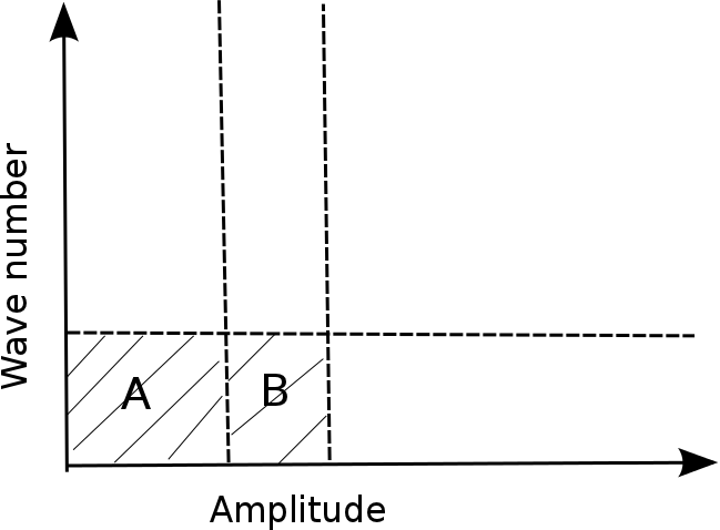
Figure 1: An illustration of the hydrodynamical expansion (small wave number) and black-hole perturbation (small amplitude). They both admit effective coupled oscillator descriptions. In AdS black-brane spacetime we compare the results from both sides of the duality, in the shaded region of the plot. For small perturbation amplitude, this comparison has been done in the linearized perturbation theory (as depicted by region “A” and see for example Kovtun and Starinets (2005)). For larger perturbation amplitude (region “B”), we are able to expand the comparison to equations of motion with nonlinear couplings using the coupled-oscillator model.

III.3 Mode expansion of the boundary fluid

We now proceed to re-write the fluid equations as a set of coupled oscillator equations so that they can be compared with the equations we will derive on the gravity side. We denote the four velocity $u^{\mu}=(\gamma,{\bf u})$, where $\gamma^{2}=1+{\bf u}\cdot{\bf u}$, and the density $\rho=\rho_{0}e^{\xi}$. Keeping viscous terms to linear order in $\bf u$ and $\xi$, and inviscid terms to quadratic order (as needed for the comparison), the energy conservation and Euler equations reduce to

$$0 = \partial_{t}\xi+{\bf u}\cdot\nabla\xi+\frac{d}{d-1}(\partial_{t}\gamma+\nabla\cdot{\bf u})\,,$$ (51)

$$0 = \partial_{t}{\bf u}+{\bf u}\cdot\nabla{\bf u}+\frac{1}{d}\nabla\xi-\frac{1}{d-1}(\partial_{t}\gamma+\nabla\cdot{\bf u}){\bf u}$$ (52)

$$-\frac{\eta}{\rho_{0}}\left(\frac{d-1}{d}\nabla^{2}{\bf u}+\frac{d-3}{d}\nabla(\nabla\cdot{\bf u})\right)\,.$$

Furthermore, dropping nonlinear terms,

$$0 = \partial_{t}\xi^{(1)}+\frac{d}{d-1}\nabla\cdot{\bf u}^{(1)}\,,$$ (53)

$$0 = \partial_{t}{\bf u}^{(1)}+\frac{1}{d}\nabla\xi^{(1)}$$ (54)

$$-\frac{\eta}{\rho_{0}}\left(\frac{d-1}{d}\nabla^{2}{\bf u}^{(1)}+\frac{d-3}{d}\nabla(\nabla\cdot{\bf u}^{(1)})\right)\,.$$

Linearized solutions are decomposed into two families of modes: sound and shear. A sound wave of momentum $\bf k$ takes the form

$${\bf u}^{(1)}_{b}\sim A_{b}({\bf k})e^{-i\omega_{b}t}e^{i{\bf k}\cdot{\bf x}}\hat{\bf k}\,,\quad\xi^{(1)}\sim B_{b}({\bf k})e^{-i\omega_{b}t}e^{i{\bf k}\cdot{\bf x}}\,.$$ (55)

By solving the linearized equations (53) and (54), the dispersion relation is found to be

$$\omega_{b}=\pm\frac{k}{\sqrt{d-1}}-i\frac{d-2}{d}\frac{\eta}{\rho_{0}}k^{2}+O(k^{3})\,,$$ (56)

and

$$B_{b}({\bf k})=\frac{d}{d-1}\frac{k}{\omega_{b}}A_{b}({\bf k})\,.$$ (57)

For the shear modes, $\xi^{(1)}=0$ and

$${\bf u}^{(1)}_{s}\sim A_{s}({\bf k})e^{-i\omega_{s}t}e^{i{\bf k}\cdot{\bf x}}\hat{\bf u}_{s}\,,$$ (58)

with $\hat{\bf u}_{s}\cdot{\bf k}=0$. The resulting dispersion relation is

$$\omega_{s}=-i\frac{d-1}{d}\frac{\eta}{\rho_{0}}k^{2}+O(k^{3})\,,$$ (59)

so shear modes are purely decaying. The general solution to the linearized fluid equations is simply a sum over sound and shear modes of different $\bf k$ and shear polarizations $s$.

We are now in a position to include the effects of nonlinear coupling terms. To do so, we express $\xi$ and $\bf u$ as sums over linear modes, but we allow for the coefficients $A$ and $B$ to be functions of time. The velocity ansatz then takes the form

$${\bf u}({\bf x},t)=\sum_{\bf k}\left[q_{b}({\bf k},t)\hat{\bf k}+\sum_{s}q_{s}({\bf k},t)\hat{\bf u}_{s}\right]e^{i{\bf k}\cdot{\bf x}}\,,$$ (60)

where $q_{s}({\bf k},t)=A_{s}({\bf k},t)e^{-i\omega_{s}t}$ and $q_{b}({\bf k},t)=A_{b}({\bf k},t)e^{-i\omega_{b}t}$. The coefficients are of course subject to a reality condition. Inserting this expansion into Eq. (52), and projecting it onto a particular shear mode, we obtain

$$\partial_{t}A_{s}({\bf k},t)$$

$$= i\sum_{{\bf p}+{\bf q}={\bf k},\,s^{\prime},\,{s^{\prime\prime}}}[\hat{\bf u}_{s^{\prime}}({\bf p},t)\cdot{\bf q}][\hat{\bf u}_{s}({\bf k},t)\cdot\hat{\bf u}_{s^{\prime\prime}}({\bf q},t)]A_{s^{\prime}}({\bf p},t)A_{s^{\prime\prime}}({\bf q},t)$$

$$+\sum_{{\bf p}+{\bf q}={\bf k},\,s^{\prime}}(\cdots)A_{s^{\prime}}({\bf p},t)q_{b}({\bf q},t)+\sum_{{\bf p}+{\bf q}={\bf k}}(\cdots)q_{b}({\bf p},t)q_{b}({\bf q},t)\,,$$

Notice that the left hand side has been reduced to simply the time derivative of $A_{s}$ because the mode function satisfies the linearized equation of motion. The right hand side describes the nonlinear coupling between modes.

The second and third terms (coupling coefficients unspecified) in Eq. (III.3) describe the mixing between the sound modes and the shear modes, as well as between two sound modes. The coefficients to these terms contain fast [$\exp(i\omega t)$ type] oscillatory time-dependent factors, so their effects tend to average to zero during the longer time scales in which we examine the growth and decay of modes. On the other hand, the first term describes the mixing between two shear modes, and it trivially satisfies the “resonant condition” in the time-domain since $\Re(\omega_{s})=0$. This results in significant energy transfer between shear modes (and had we been performing an ordinary perturbative expansion would have resulted in secular growth). It is then natural to expect that the effect of sound modes is sub-dominant in the turbulent process of conformal fluids, where the viscous damping is less important. In fact, if we ignore all the sound modes in the relativistic hydro equation, the resulting Eq. (III.3) is the same as the one for incompressible fluid (Appendix B), and they share the same conservation laws in the Fourier domain.

Equation (III.3) expresses the fluid as a collection of coupled oscillators, to be compared with (28) on the gravity side. In the next section we shall apply the general formalism of Sec. II to the AdS black brane spacetime and directly match its mode coupling coefficients (for the fundamental hydro shear quasinormal modes) to the shear-shear mode coupling coefficients in Eq. (III.3). One can apply the same procedure to verify the correspondence in the sound channel (which we have not written down). We will only address the shear modes, as the main purpose of this work is to formulate the coupled oscillator model and to illustrate its technical details, rather than to provide a full verification of the gravity/fluid correspondence. We envisage that this framework shall prove its unique value when studying gravitational interactions in spacetime without a clear gravity/fluid correspondence, or in cases where the hydrodynamical (long-wavelength) approximation becomes too restrictive.

IV Linear and nonlinear gravitational perturbations of the AdS₅ black-brane

In this section we study gravitational perturbations about an asymptotically AdS black brane within the context of the coupled oscillator model. We adopt this particular example for two reasons: On the one hand, the boundary metric of the background spacetime is flat, which simplifies calculations when performing wave function projections. On the other hand, the gravity/fluid correspondence is well established in this spacetime, and this allows us to compare results obtained in the gravity and dual fluid pictures, as depicted in Fig. 1. In particular, we shall focus on the analysis of shear modes at both linear and nonlinear levels. We also fix the spacetime dimension to $d+1=5$, although it is straightforward to generalize the analysis below to other dimensions. For calculations within this section, we make further simplifications by scaling the coordinates such that $b=1$, so the horizon is located at $r=1$. This means that we effectively choose $T=1/\pi$ so [see above Eq. (III.1)]

$$x^{i}=\frac{1}{2}\tilde{x}^{i}\,,\quad k_{i}=2\tilde{k}_{i}\,.$$ (62)

IV.1 Linear perturbation

Linear quasinormal mode perturbations of AdS black branes have been thoroughly analyzed in Kovtun and Starinets (2005). There, the fundamental (slowly decaying) quasinormal modes of the spacetime were shown to be the same as the hydrodynamical modes of the boundary fluid. The analysis was performed using the coordinate system of Eq. (III.1), whereas for our purposes it is more convenient to use the ingoing coordinates of Eq. (32). As discussed in Appendix C, choosing different coordinates leads to different definitions for the modes. At the linear level there exists a clean one-to-one mapping of modes in different bases as each quasinormal mode is a solution to the linear Einstein equation. However, when studying nonlinear perturbations, their projection with respect to a mode-basis associated to a different coordinate system leads to an expansion with a less direct identification. In Appendix C we illustrate this point with a simple example describing a scalar field propagating on Minkowski spacetime.

As demonstrated in Kovtun and Starinets (2005), linear perturbations of the AdS black brane can be classified into shear, sound and scalar sectors. In addition, as the boundary metric is flat, it is straightforward to Fourier transform the metric components along the boundary coordinates. The same logic applies when we adopt ingoing coordinates. Without loss of generality, we consider a mode whose boundary-coordinate dependence is $e^{ikz}$. For shear perturbations, the relevant metric components are then $h_{r\alpha},h_{v\alpha},h_{z\alpha}$, where $\alpha=x,y$. Without loss of generality, we choose the polarization $\alpha=x$, and impose the radial gauge condition $h_{rM}=0$, with $M=\{r,v,z,x,y\}$. Defining the auxiliary variables

$$H_{zx}\equiv h_{zx}\frac{e^{-ikz}}{r^{2}},\quad H_{vx}\equiv h_{vx}\frac{e^{-ikz}}{r^{2}}\,,$$ (63)

the independent components of the linearized Einstein equation take the form

$$0 = 5r\frac{\partial H_{vx}}{\partial r}+ik\frac{\partial H_{zx}}{\partial r}+r^{2}\frac{\partial^{2}H_{vx}}{\partial r^{2}}\,,$$ (64)

$$0 = k^{2}H_{vx}-5r^{3}f\frac{\partial H_{vx}}{\partial r}-r^{4}f\frac{\partial^{2}H_{vx}}{\partial r^{2}}+ik\frac{\partial H_{zx}}{\partial v}-r^{2}\frac{\partial^{2}H_{vx}}{\partial v\partial r}\,.$$

We can further simplify this system by defining the master variable, $\Psi\equiv\partial_{r}H_{vx}$. This satisfies the master equation,

$$-k^{2}\Psi+(5r^{3}f\Psi)^{\prime}+(r^{4}f\Psi^{\prime})^{\prime}+7r\dot{\Psi}+2r^{2}\dot{\Psi}^{\prime}=0\,,$$ (65)

where in this section we will often denote partial derivatives as $(\cdot)^{\prime}\equiv\partial_{r}$ and $\dot{(\cdot)}\equiv\partial_{v}$. To look for quasinormal modes, we first take advantage of the time translation symmetry of the equation to impose a $e^{-i\omega v}$ time dependence (so $\dot{\Psi}\to-i\omega\Psi$). Solving the remaining spatial equation with appropriate boundary conditions at the horizon and spatial infinity gives rise to a set of quasinormal modes in the ingoing coordinates, and the frequency spectrum $\omega(k)$.

To analyze the horizon boundary, we multiply Eq. (65) by $f$ and take the horizon limit $r\rightarrow 1$. The wave equation becomes

$$(\partial^{2}_{r_{*}}+2\partial_{v}\partial_{r_{*}})\Psi=0\,,$$ (66)

with two independent solutions,

$$\partial_{r_{*}}\Psi=0,\quad{\rm and}\quad(\partial_{r_{*}}+2\partial_{v})\Psi=0\,.$$ (67)

The ingoing boundary condition for the quasinormal modes selects

$$\frac{\partial\Psi}{\partial r_{*}}\to 0,\quad r\rightarrow 1\,.$$ (68)

As $r\to\infty$ we impose a reflecting boundary condition (since the spacetime is asymptotically AdS), so the metric perturbation is required to vanish. This means that we should at least expect $h=O(1/r)$ and $\Psi=O(1/r^{4})$.

The above discussion applies to all quasinormal modes of our system. However, the dual fluid captures only the longest lived shear and sound modes, which have $\omega\to 0$ as $k\to 0$ (known as the “hydro” modes). In order to compare our results with the fluid we therefore restrict to $\tilde{k}\ll 1$. We can then construct the eigenfunctions perturbatively in $k$ (and $\omega$). In this expansion, the leading order part of equation (65) is

$$(5r^{3}f)^{\prime}\Psi+5fr^{3}\Psi^{\prime}+r^{4}f\Psi^{\prime\prime}+(r^{4}f)^{\prime}\Psi^{\prime}=0\,.$$ (69)

After imposing the horizon boundary condition, the solution is

$$\Psi_{0}=\frac{C(v)}{r^{5}}\,.$$ (70)

where the subscript $0$ indicates that this solves the leading order equation. (Notice that this solution also falls off sufficiently rapidly at spatial infinity.) To look for quasinormal mode solutions we take $C(v)=e^{-i\omega v}$.

The leading order solution $\Psi_{0}$ then sources the first order correction $\Psi_{1}$ through

$$(5r^{3}f)^{\prime}\Psi_{1}+5fr^{3}\Psi_{1}^{\prime}+r^{4}f\Psi_{1}^{\prime\prime}+(r^{4}f)^{\prime}\Psi_{1}^{\prime}$$

$$=-(-k^{2}\Psi_{0}+7r\dot{\Psi}_{0}+2r^{2}\dot{\Psi}^{\prime}_{0})\,.$$ (71)

The combined solution $\Psi=\Psi_{0}+\Psi_{1}$ is then

$$\Psi= \left[\frac{1}{r^{5}}+\frac{-(k^{2}-4i\omega)\log(1-r)-(k^{2}+4i\omega)\log(1+r)}{16r^{5}}\right.$$

$$\left.+\frac{8i\omega\arctan r+k^{2}\log(1+r^{2})}{16r^{5}}\right]e^{-i\omega v}\,.$$ (72)

In order to satisfy the horizon boundary condition we must impose $k^{2}=4i\omega$, resulting in

$$\Psi=\left[\frac{1}{r^{5}}+\frac{2k^{2}\arctan r-2k^{2}\log(1+r)+k^{2}\log(1+r^{2})}{16r^{5}}\right]e^{-i\omega v}\,.$$ (73)

Using Eq. (62), we verify that $k^{2}=4i\omega$ is equivalent to $\tilde{\omega}=-i\tilde{k}^{2}/2$, which is exactly the dispersion relation of shear hydro quasinormal modes derived in Kovtun and Starinets (2005) using a different coordinate system. In addition, it is easy to check that the dispersion relation matches (59), derived on the fluid side.

Knowing $\Psi$, it is straightforward to use Eq. (64) to reconstruct the metric perturbations. For the shear modes considered here, the metric perturbation is

$$h_{vx} = -\frac{A}{4r^{2}}e^{-i\omega v+ikz}\left[1+\frac{k^{2}r^{2}}{16}(\pi r^{2}-4r+2)\right.$$

$$\quad\left.-\frac{k^{2}}{16}(r^{4}-1)\left(2\arctan r+\log\frac{1+r^{2}}{(1+r)^{2}}\right)\right]\,,$$

$$h_{zx} = i\frac{A}{4}kr^{2}e^{-i\omega v+ikz}\left[\frac{\pi}{4}-\frac{1}{r}-\frac{\arctan r}{2}\right.$$ (75)

$$\quad\left.+\frac{1}{4}\log\frac{(1+r^{2})(1+r)^{2}}{r^{4}}\right]\,.$$

IV.2 Mode projection

Having carried out the linear analysis, we are almost ready to calculate the shear-shear mode coupling coefficient. There is one more problem to tackle however, which is to project the Einstein equation onto an individual mode to see how a source term affects its evolution. As described in Sec. II.3, we adopt a technique that has been proven very powerful in solving similar problems Leung et al. (1997, 1999); Yang et al. (2015); Mark et al. (2015); Yang and Zhang (2014); Zimmerman et al. (2014). Namely, we enlist a suitable bilinear form to project the equation onto individual modes.

For later convenience, we define $\phi=r^{5}\Psi$, so that Eq. (65) takes the form

$$\left(\frac{f}{r}\phi^{\prime}\right)^{\prime}-k^{2}\frac{\phi}{r^{5}}+\frac{7}{r^{4}}\dot{\phi}+2r^{2}\left(\frac{\dot{\phi}}{r^{5}}\right)^{\prime}=0\,.$$ (76)

Fourier transforming the wave operator in $v$, we define

$$H_{\omega}\phi\equiv\left(\frac{f}{r}\phi^{\prime}\right)^{\prime}-k^{2}\frac{\phi}{r^{5}}-\frac{7i\omega}{r^{4}}\phi-2i\omega r^{2}\left(\frac{\phi}{r^{5}}\right)^{\prime}\,.$$ (77)

We also define a generalized inner product,

$$\langle\chi|\eta\rangle=\int^{\infty}_{1}dr\chi\,\eta\,.$$ (78)

The operator $H_{\omega}$ is not symmetric under this bilinear form, i.e., $\langle\chi|H_{\omega}\eta\rangle\neq\langle H_{\omega}\chi|\eta\rangle$, because of the fourth term in $H_{\omega}$. However, in the hydrodynamic limit ($\tilde{k}\ll 1$) this term is neglected, so (78) is suitable for our purpose of comparing to the dual fluid.

For completeness, we note that should the need arises for the study of perturbations of higher overtones away from the hydro limit, we may use an alternative bilinear form (dependent on $\omega$) with respect to which $H_{\omega}$ is symmetric so that $\langle\chi|H_{\omega}\eta\rangle_{\omega}=\langle H_{\omega}\chi|\eta\rangle_{\omega}$. In this case,

$$\langle\chi|\eta\rangle_{\omega} = \int^{\infty}_{1}drg_{\omega}(r)\chi\,\eta\,,\quad\text{with}$$ (79)

$$\log g_{\omega}(r) = -i\omega\left(\arctan r+\frac{1}{2}\log\frac{1-r}{1+r}\right)+{\rm const}\,,$$

is the unique option. There is one $g_{\omega}$ for each $\omega$, so we have a family of such generalized inner products. Using $g_{\omega}$ to project onto the mode with frequency $\omega$ [followed by a diagonalization procedure as per the discussion above Eq. (17)] is a natural choice, and indeed leads to agreement with the Green’s function method for projecting modes (see Appendix D). In any case, to $O(k^{2})$, these generalized inner products reduce to Eq. 78.

For the purpose of the time-domain analysis in the next section, we expect the effect of non-hydrodynamical modes [see Eq. (87) below] and the excitation of residual parts to be at least $O(k)$. Therefore only the hydrodynamical modes are important to leading order and we shall adopt the generalized inner product (78) for calculations, as it is easier to implement in the time-domain analysis. As an example, we show below that this inner product generates the correct leading order (in $k$) frequency in the eigenvalue analysis.

Let us now consider a simple example that demonstrates the essence of how to utilize this inner product to carry out perturbation studies. Suppose we perturb $k$ to $k+\epsilon\delta k$ ($\epsilon\ll 1$) and ask for the change of $\omega$. On the one hand, based on the dispersion relation $\omega=-ik^{2}/4$, we immediately know that $\delta\omega=-ik\delta k/2$. On the other hand, we can arrive at the same conclusion through a perturbation analysis of the eigenvalue problem defined by Eq. (77).

The change $k\rightarrow k+\epsilon\delta k$ causes $H$ to pick up an extra term, $-2\epsilon k\delta k/r^{5}$. We expect both the eigenfrequency and the eigenfunction to also change to order $\epsilon$,

$$\phi\rightarrow\phi+\epsilon\phi^{(1)}+O(\epsilon^{2})\,,$$

$$\omega\rightarrow\omega+\epsilon\delta\omega+O(\epsilon^{2})\,.$$ (80)

Plugging into the wave equation Eq. (77), and projecting both sides onto $\phi$ while keeping only the $O(\epsilon)$ terms, we can eliminate the unknown function $\phi^{(1)}$ to obtain

$$-i\delta\omega= 2k\delta k\frac{\langle\phi|1/r^{5}\phi\rangle}{\langle\phi|7\phi/r^{4}+2r^{2}(\phi/r^{5})^{\prime}\rangle}+O(k^{2})$$

$$\approx -\frac{k}{2}\delta k\,,$$ (81)

which is consistent with our expectation. We note that it was necessary in this analysis to use the symmetry property of $H_{\omega}$ to eliminate terms involving $\phi^{(1)}$. Although somewhat excessive for this simple problem, we see that with the help of our generalized inner product, it is now possible to carry out a perturbation analysis in a manner analogous to the application of perturbation theory in quantum mechanics Shankar (1980) (for a direct mapping of a wave equation with outgoing boundary condition into a Schrödinger equation with non-Hermitian Hamiltonian, see Leung et al. (1998)).

IV.3 Nonlinear analysis

We are now in a position to move beyond the linear level and study the second order (nonlinear) Einstein equation (10). We begin by considering its projection onto the shear sector with spatial dependence $e^{ikx}$ and spatial polarization $\alpha=z$ (see Sec. IV.1). (It is straightforward to perform this projection onto a Fourier basis element with an ordinary inner product. The nontrivial aspect is the subsequent projection onto the hydro mode.) The non-vanishing $vx$ and $rx$ components of the Einstein equation take the form

$$5r\frac{\partial H_{vz}}{\partial r}+ik\frac{\partial H_{zx}}{\partial r}+r^{2}\frac{\partial^{2}H_{vz}}{\partial r^{2}}=\tau_{rz}\,,$$

$$k^{2}H_{vz}-5r^{3}f\frac{\partial H_{vz}}{\partial r}-r^{4}f\frac{\partial^{2}H_{vz}}{\partial r^{2}}+ik\frac{\partial H_{zx}}{\partial v}-r^{2}\frac{\partial^{2}H_{vz}}{\partial v\partial r}$$

$$=\tau_{vz}\,.$$ (82)

We have formally written the nonlinear terms as “sources” on the right hand side of the equation. At quadratic order the nonlinear terms are

$$\tau_{rz}\equiv-\langle e^{-ikx},2R^{(2)}_{rz}\rangle,\quad\tau_{vz}\equiv-\langle e^{-ikx},2R^{(2)}_{vz}\rangle\,.$$ (83)

The inner product $\langle\cdot,\cdot\rangle$ is the ordinary inner product over the boundary spatial coordinates. Equation (IV.3) is simply (64) with nonlinear terms included, and a simple switch of coordinates $x\leftrightarrow z$.

Since the second order Ricci tensor is a quadratic function of the metric perturbation, which can be expanded over Fourier modes (and scalar, sound, shear sectors), the projection (83) enforces a wave number matching condition on the terms that can contribute to the right hand side of (IV.3). Namely, modes with wave numbers ${\bf p}$ and ${\bf q}$ can only act as a source for mode ${\bf k}$ if ${\bf p}+{\bf q}={\bf k}$ (see Fig. 2). [This of course also holds for the fluid analysis in (III.3).] We define the angles $\theta_{1}\equiv\arccos(\hat{q}\cdot\hat{k})$ and $\theta_{2}\equiv\arccos(\hat{p}\cdot\hat{k})$.

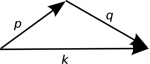
Figure 2: An illustration of three wave numbers satisfying the “momentum matching” condition.

Following the same procedure as in the linear analysis, we re-write Eq. (IV.3) in the form of a sourced version of Eq. (76),

$$\left(\frac{f}{r}\phi^{\prime}\right)^{\prime}-k^{2}\frac{\phi}{r^{5}}+\frac{7}{r^{4}}\dot{\phi}+2r^{2}\left(\frac{\dot{\phi}}{r^{5}}\right)^{\prime}$$ (84)

$$= -\dot{\tau}_{rz}-\tau_{vz}^{\prime}\equiv S_{\rm in}\,.$$

Since only first order time derivatives appear in this wave equation and we know from the previous subsection that the quasinormal frequency is purely imaginary, this shear hydrodynamic mode belongs to the class described by Eq. (29).

We now proceed to compute the nonlinear source $S_{j}$ [see (29)] using the generalized inner product of Sec. IV.2. As in Sec. II.3, we first express the field $\phi$ as a sum over radial modes

$$\phi\to A_{0}(t)e^{-i\omega_{0}v}\chi_{0}(r)+\sum_{j>0}A_{j}(t)e^{-i\omega_{j}v}\chi_{j}(r)+O(k)\,,$$ (85)

but we allow for the modes to have additional time dependence through the mode amplitudes $A_{j}$. Here the spatial wavefunctions are denoted $\chi_{j}$, with $j=0$ corresponding to the hydro mode. The non-hydro modes all have frequencies $\omega_{j}=O(1)$, while $\omega_{0}=-ik^{2}/4$. While $\phi$ is to be matched to modes of the $4$-velocity $u^{\mu}$ on the fluid side, we normalize the wave function

$$\chi_{0}=4$$ (86)

accordingly . The $O(k)$ appearing in the expression for $\phi$ includes the residual contribution under the hydrodynamical approximation (see Footnote 4).

We can now plug (85) into the wave equation (84), and then take the generalized inner product of both sides with $\chi_{0}$ using (78). Within this computation, the effect of the non-hydrodynamical terms is at least $O(k)$ [in fact $O(k^{2})$] as we claimed in Sec. IV.2. This is because $e^{-i\omega_{j}v}\chi_{j}$ solves the linear equation (76), so for $j>0$

$$\omega_{j}\left\langle\chi_{0}\left|\frac{7}{r^{4}}\chi_{j}+2r^{2}\left(\frac{\chi_{j}}{r^{5}}\right.\right)^{\prime}\right\rangle$$ (87)

$$= -\left\langle\chi_{0}\left|\left(\frac{f}{r}\chi_{j}^{\prime}\right)^{\prime}-k^{2}\frac{\chi_{j}}{r^{5}}\right.\right\rangle$$

$$= -\left\langle\left(\left.\frac{f}{r}\chi_{0}^{\prime}\right)^{\prime}-k^{2}\frac{\chi_{0}}{r^{5}}\right|\chi_{j}\right\rangle$$

$$= \omega_{0}\left\langle\left.\frac{7}{r^{4}}\chi_{0}+2r^{2}\left(\frac{\chi_{0}}{r^{5}}\right)^{\prime}\right|\chi_{j}\right\rangle$$

$$= O(k^{2})\,.$$

Given this observation, it is now simple to show that

$$\dot{A} \approx \frac{1}{4}\frac{\langle\chi_{0}|S_{\rm in}\rangle e^{i\omega_{0}v}}{\langle\chi_{0}|7\chi_{0}/r^{4}+2r^{2}(\chi_{0}/r^{5})^{\prime}\rangle}$$ (88)

$$\approx -\frac{1}{4}\tau_{vz}|_{r=1}\,,$$

where we dropped high order [$O(k^{2})$ and higher] terms in $k$, including nonlinear terms containing time derivatives (as discussed in Sec. II.3). Using Eq. (II.1), the mode expansion of $h_{\mu\nu}$, and after some lengthy but nevertheless straightforward calculations, one can show that the shear-shear mode coupling coefficient arising from (88) is

$$\kappa_{kpq} = ik\sin(\theta_{2}-\theta_{1})\,,$$ (89)

which agrees with the result obtained with its fluid counterpart from Eq. (III.3)

$$\kappa_{kpq}=i[\hat{\bf u}_{s^{\prime}}({\bf p},t)\cdot{\bf q}][\hat{\bf u}_{s}({\bf k},t)\cdot\hat{\bf u}_{s^{\prime\prime}}({\bf q},t)]+({\bf p}\leftrightarrow{\bf q})\,.$$ (90)

We end this section by noting that the agreement between the mode coupling coefficients inferred from the fluid equations and the AdS black brane perturbation theory relies on the fact that they are computed using the same mode basis, and that the comparison is made in the regime where $\tilde{k}\ll 1$ and $|h|\ll 1$ (cf. Fig. 1). However, the coupled oscillator model is applicable more broadly.

V Conclusions

The study of nonlinear wave phenomena is undoubtedly a fascinating subject. Gaining understanding in the particular case of general relativity poses unique challenges even given the fixed speed of propagation of physical perturbations. These challenges are rooted in the covariant nature of the theory and physical degrees of freedom often hidden within a larger set of (metric) variables. These issues have hampered understanding of gravitational perturbations beyond linear order except in a few specialized regimes Gleiser et al. (2000); Ioka and Nakano (2007); Brizuela et al. (2009); Pound (2012); Gralla (2012), seamingly leaving full numerical simulations as the main tool to try to understand these issues (for a recent overview of these efforts, see Choptuik et al. (2015) and references cited therein).

In the current work, we have presented a model to capture the nonlinear behavior of gravitational perturbations. This model regards the system as composed of a collection of nonlinearly coupled (damped) harmonic oscillators with characteristic (isolated) frequencies given by quasinormal modes. By construction this model reproduces standard results obtained at the linearized level. At the nonlinear level, it describes mode-mode couplings and their effect on frequency and amplitude shifts. As an illustration, we have shown how our model reproduces recent results captured through the gravity/fluid correspondence via a purely gravitational calculation. Importantly, the applicability of our formalism is not restricted to long-wavelength perturbations—as in the case of the gravity/fluid correspondence—so the coupled oscillator model can also treat so-called “fast (non-hydrodynamical) modes” of perturbed black holes Friess et al. (2007). As a consequence it can be employed to study a broder phenomenology than that reachable via the correspondence. We stress that our formalism is also applicable beyond asymptotically AdS spacetimes. Thus it can also help shed light on nonlinear mode generation in perturbations of asymptotically flat black hole spacetimes Papadopoulos (2002); Zlochower et al. (2003).

Appendix A Brief overview of coupled oscillator systems

Consider a family of nonlinearly coupled harmonic oscillators governed by,

$$\ddot{q}_{j}+\gamma_{j}\dot{q}_{j}+\tilde{\omega}^{2}_{j}q_{j}$$

$$=\sum_{kl}(\tilde{\lambda}^{(1)}_{jkl}q_{k}q_{l}+\tilde{\lambda}^{(2)}_{jkl}\dot{q}_{k}q_{l}+\tilde{\lambda}^{(3)}_{jkl}\dot{q}_{k}\dot{q}_{l})\equiv S_{j}\,,$$ (91)

where $\tilde{\omega}^{2}_{j}q_{j}$ is the restoring force and $\gamma_{j}$ is the damping coefficient. Each oscillator’s displacement can be decomposed in the same way as Eq. (14), with $\omega_{j}$ satisfying

$$-\omega^{2}_{j}-i\gamma_{j}\omega_{j}+\tilde{\omega}^{2}_{j}=0\,.$$ (92)

In the presence of nonlinear mode-mode coupling ($\tilde{\lambda}^{(n)}_{jkl}\neq 0$), $A_{j}$ and $B_{j}$ are both time-dependent. In fact, we can take one more time derivative of the first equation in Eq. (II.3.2) , and obtain

$$(\dot{A}_{j}-i\omega_{j}A_{j})e^{-i\omega_{j}t}=\frac{1}{\omega_{j}+\omega^{*}_{j}}(\omega^{*}_{j}\dot{q}_{j}+i\ddot{q}_{j})$$

$$=\frac{iS_{j}}{\omega_{j}+\omega^{*}_{j}}+\left(\frac{\dot{q}_{j}\omega_{j}^{*}}{\omega_{j}+\omega^{*}_{j}}+\frac{\gamma_{j}\dot{q}_{j}+\tilde{\omega}^{2}_{j}q_{j}}{i(\omega^{*}_{j}+\omega_{j})}\right)\,,$$

$$=\frac{iS_{j}}{\omega_{j}+\omega^{*}_{j}}-\frac{i\omega_{j}}{\omega_{j}+\omega^{*}_{j}}(\omega^{*}_{j}q_{j}+i\dot{q}_{j})\,,$$ (93)

such that

$$\dot{A}_{j}=\frac{iS_{j}}{\omega_{j}+\omega^{*}_{j}}e^{i\omega_{j}t}\,,$$ (94)

and similarly

$$\dot{B}_{j}=-\frac{iS_{j}}{\omega_{j}+\omega^{*}_{j}}e^{-i\omega^{*}_{j}t}\,.$$ (95)

These effective equations of motion have the same kind of first-order form as Eq. (29) and Eq. (28), which means that one can utilize results from previous studies on nonlinear coupled oscillators to analyze nonlinear gravitational interactions.

Appendix B Two-dimensional incompressible fluid in the inertial regime

Here we review the Navier-Stokes equation for a two-dimensional incompressible fluid. This discussion highlights how a new symmetry for the mode-mode coupling coefficient arises in the mode-expansion picture. Such symmetry is critical for the double-cascading (inverse energy and direct enstrophy cascades) behavior in two-dimensionalfluids. A more detailed discussion can be found in Ref. Kraichnan (1967).

The Navier-Stokes equation for an incompressible fluid in the spatial-frequency domain reads

$$\left(\frac{\partial}{\partial t}+\nu k^{2}\right)u_{j}({\bf k},t)$$

$$=ik_{l}P_{jn}({\bf k})\sum_{{\bf p}+{\bf q}={\bf k}}u_{n}({\bf p},t)u_{l}({\bf q},t)\,$$

$$=\frac{ik_{l}P_{jn}({\bf k})}{2}\sum_{{\bf p}+{\bf q}={\bf k}}[u_{n}({\bf p},t)u_{l}({\bf q},t)+u_{n}({\bf q},t)u_{l}({\bf p},t)]\,$$ (96)

where ${\bf u}({\bf x},t)=\sum_{{\bf k}}e^{i{\bf k}\cdot{\bf x}}{\bf u}({\bf k},t)$ and $P_{jn}({\bf k})\equiv\delta_{jn}-k_{j}k_{n}/k^{2}$. In incompressible fluids, the condition $\nabla\cdot{\bf u}=0$ translates to ${\bf k}\cdot{\bf u}({\bf k},t)=0$ in the Fourier domain. We can write ${\bf u}({\bf k},t)$ as

$${\bf u}({\bf k},t)=A({\bf k},t){\hat{u}}({\bf k},t)\,,$$ (97)

where $\hat{u}({\bf k},t)$ satisfies $\hat{u}\cdot{\bf k}=0$ and $\hat{u}\cdot\hat{u}=1$. In $2+1$ fluids, $\hat{u}$ is unique for any ${\bf k}$. Using the new variables, the Navier-Stokes equation can be rewritten as

$$\left(\frac{\partial}{\partial t}+\nu k^{2}\right)A({\bf k},t) =i\sum_{{\bf p}+{\bf q}={\bf k}}\kappa({\bf k},{\bf p},{\bf q})A({\bf p},t)A({\bf q},t)\,$$

$$=i\sum_{{\bf p}+{\bf q}={\bf k}}\{[\hat{u}({\bf k},t)\cdot\hat{u}({\bf p},t)][{\bf k}\cdot\hat{u}({\bf q},t)]+[\hat{u}({\bf k},t)\cdot\hat{u}({\bf q},t)][{\bf k}\cdot\hat{u}({\bf p},t)]\}A({\bf p},t)A({\bf q},t)\,.$$ (98)

This is the same as the shear-shear coupling term in Eq. (III.3), which is already written in a form consistent with the coupled oscillator model.

In the inertial regime we shall set the viscosity coefficient $\nu$ to zero (as such coefficient only governs the extent of the regime but not the behavior within it) and recall that ${\bf u}({\bf x},t)$ must be real. One can then show that

$$-\frac{\partial[u_{j}({\bf k},t)u^{*}_{j}({\bf k},t)]}{\partial t}=\sum_{{\bf p}+{\bf q}+{\bf k}=0}{\rm Im}\{[{\bf u}({\bf k},t)\cdot{\bf u}({\bf p},t)][{\bf k}\cdot{\bf u}({\bf q},t)]+[{\bf u}({\bf k},t)\cdot{\bf u}({\bf q},t)][{\bf k}\cdot{\bf u}({\bf p},t)]\}$$

$$\equiv\sum_{{\bf p}+{\bf q}+{\bf k}=0}{\rm Im}[\kappa({\bf k},{\bf p},{\bf q})A({\bf p},t)A({\bf q},t)A({\bf k},t)]\,.$$ (99)

Energy conservation requires that

$$\frac{\partial[u_{j}({\bf k},t)u^{*}_{j}({\bf k},t)]}{\partial t}+\frac{\partial[u_{j}({\bf p},t)u^{*}_{j}({\bf p},t)]}{\partial t}+\frac{\partial[u_{j}({\bf q},t)u^{*}_{j}({\bf q},t)]}{\partial t}=0\,,$$ (100)

which is equivalent to demanding

$$\kappa({\bf k},{\bf p},{\bf q})+\kappa({\bf q},{\bf k},{\bf p})+\kappa({\bf p},{\bf q},{\bf k})=0$$ (101)

for any vectors ${\bf k}$, ${\bf p}$, and ${\bf q}$ satisfying ${\bf p}+{\bf q}+{\bf k}=0$. It is straightforward to check that the above relation is automatically satisfied given the expression of $\mathcal{T}$. Moreover, for $2+1$ fluids, by using the fact that ${\bf k}\cdot{\bf u}({\bf k},t)={\bf p}\cdot{\bf u}({\bf p},t)={\bf q}\cdot{\bf u}({\bf q},t)=0$ and the identity

$$\sin^{3}\theta_{1}\cos(\theta_{2}-\theta_{3})+\sin^{3}\theta_{2}\cos(\theta_{3}-\theta_{1})+\sin^{3}\theta_{3}\cos(\theta_{1}-\theta_{2})=0\,,$$ (102)

for $\forall\theta_{1}+\theta_{2}+\theta_{3}=\pi\,,$ we can show that an additional symmetry for the mode-mode coupling exists, which is

$$k^{2}\kappa({\bf k},{\bf p},{\bf q})+q^{2}\kappa({\bf q},{\bf k},{\bf p})+p^{2}\kappa({\bf p},{\bf q},{\bf k})=0\,.$$ (103)

This additional symmetry is directly connected with the additional conserved quantity in $2+1$ fluids: enstrophy. With two conserved quantities in the inertial regime, Kraichnan Kraichnan (1967) explained that a dual-cascading behavior should be expected in the turbulent regime. This example strongly suggests that the symmetry of the mode-mode coupling coefficients in our coupled oscillator model could be crucial for classifying the nonlinear behavior of gravitational evolutions.

Appendix C Expansion in two different bases

Let us imagine a simple example of a scalar field whose perturbations propagate on a 2-dimensional flat spacetime with time-like boundaries at $x=0$ and $x=1$. For comparison purposes, we have assigned two coordinate systems in this spacetime: standard Cartesian coordinates $(t,x)$ and “null” $(v,x)$ coordinates, with $v\equiv t+x$. For simplicity, we impose Dirichlet boundary conditions $\Phi|_{x=0}=\Phi|_{x=1}=0$ for the wave. At linear order, the scalar wave satisfies the following wave equation

$$(-\partial^{2}_{t}+\partial^{2}_{x})\Phi=0\,,$$ (104)

in the $(t,x)$ coordinate system or

$$(\partial^{2}_{x}+2\partial_{v}\partial_{x})\Phi=0\,,$$ (105)

in the $(v,x)$ coordinate system.

Based on the wave equation and the boundary conditions, we can see that this is a standard Sturm-Liouville problem, where it is straightforward to write down the solutions of the wave equation in a mode expansion

$$\Phi(t,x)=\sum_{j}\left(A_{j}e^{-i\omega_{j}t}+B_{j}e^{i\omega_{j}t}\right)\sin(j\pi x)\,,$$ (106)

and

$$\Phi(v,x)=\sum_{j}\left(\tilde{A}_{j}e^{-i\omega_{j}v}e^{i\omega_{j}x}+\tilde{B}_{j}e^{i\omega_{j}v}e^{-i\omega_{j}x}\right)\sin(j\pi x)\,,$$ (107)

with $\omega_{j}=j\pi$. It is obvious that we can match up the linear modes from the two different expansions above, and in fact we can make the identifications

$$A_{j}=\tilde{A}_{j},\quad B_{j}=\tilde{B}_{j}\,.$$ (108)

Figure 3: An illustration for mode decompositions of a scalar field in a flat spacetime. At each point (such as the star in the diagram), we show two possible mode bases with respect to which to decompose the scalar wave.

Now suppose nonlinear terms ($\Phi^{2}$, $\Phi^{3}$ or even higher order) are present in the wave equations, resulting in a new solution [$\Phi(t,x)$ or $\Phi(v,x)$]. For such a wave, we can still choose constant-$t$ or constant-$v$ slices, and use the above spatial mode basis to perform a decomposition

$$\Phi(t,x)=\sum_{j}\left[A_{j}(t)e^{-i\omega_{j}t}+B_{j}(t)e^{i\omega_{j}t}\right]\sin(j\pi x)\,,$$ (109)

in the $(t,x)$ coordinates, and

$$\Phi(v,x)=\sum_{j}\left[\tilde{A}_{j}(v)e^{-i\omega_{j}v}e^{i\omega_{j}x}+\tilde{B}_{j}(v)e^{i\omega_{j}v}e^{-i\omega_{j}x}\right]\sin(j\pi x)$$ (110)

in the $(v,x)$ coordinates. We note that the mode amplitudes are generically time-dependent now.

Pick an arbitrary point in the spacetime (for example, the one labeled with a “star” in Fig. 3). There we can ask whether the matching described in Eq. (108) still holds for the two different mode expansions at that point. As we can see from Fig 3, these two mode expansions sample two different slices of the spacetime: one at constant $t$ and the other at constant $v$. Unlike the linear case, the scalar wave distributions on these two slices can be made quite “independent” of each other by freely detuning the nonlinear terms in the wave equations. In the end, the largely independent data on these two slices imply that simple mappings such as Eq. (108) no longer exist for mode expansions under different bases in the general nonlinear scenario. However, we emphasize that despite the lack of a simple mapping between them, both mode expansions are equally valid in describing the wave evolution. Although our present analysis is performed using this simple example where the mode expansion is complete, we see no reason why a similar conclusion would not hold for quasinormal mode expansions of generic spacetimes.

Appendix D Coupled oscillator model in Schwarzschild spacetime

As discussed in Sec. II, generic linear metric perturbations can be decomposed into quasinormal modes plus a residual part. Unless we are dealing with normal modes which form a complete basis, or under certain physical conditions in which quasinormal modes dominate (e.g., AdS perturbations in the hydrodynamical limit), ignoring the contribution from the residual part should always require justification. Here we offer an alternative way of arriving at the coupled oscillator model, using the Green’s function approach (see also Barranco et al. (2014)). Using this method, the quasinormal mode excitations can be unambiguously determined given a driving source term. So far this approach can only be demonstrated for perturbations with separable wave equations, such as Schwarzschild and Kerr perturbations, and we shall leave extensions to more general spacetimes to future studies.

To simplify the problem, we assume that the angular dependence has been factored out, and we focus on the nonlinear evolution of modes with spherical harmonic indices $(l,m)$, which satisfy the Regge-Wheeler (odd partity) and Zerilli-Moncrief (even parity) wave equations

$$\left[-\frac{\partial^{2}}{\partial t^{2}}+\frac{\partial^{2}}{\partial r^{2}_{*}}+V_{\rm e/o}(r)\right]\Psi_{\rm e/o}=S_{\rm e/o}(r,t)\,.$$ (111)

Here $r_{*}\equiv r+2M\log[r/(2M)-1]$ and $\Psi_{\rm e},\Psi_{\rm o}$ are the Zerelli-Moncrief and Regge-Wheeler gauge invariant quantities, respectively. The expressions for the potential $V_{\rm e/o}$ and angular-projected source $S_{\rm e/o}$ can be found in Martel and Poisson (2005); Yang et al. (2014). In our present study, $S_{\rm e/o}$ is defined by the second order Ricci tensor, which is bilinear in the metric perturbations.

Without the source term, for fixed time dependence $e^{-i\omega t}$ there are two independent solutions to each wave equation. One solution asymptotes to

$$u_{\rm in}\rightarrow e^{-i\omega(t+r_{*})},\quad r_{*}\rightarrow-\infty$$ (112)

near the event horizon, and

$$u_{\rm in}\rightarrow C_{\rm in}(\omega)e^{-i\omega(t+r_{*})}+C_{\rm out}(\omega)e^{-i\omega(r-r_{*})},\quad r_{*}\rightarrow\infty$$ (113)

at spatial infinity. The other solution satisfies

$$u_{\rm out}\rightarrow e^{-i\omega(t-r_{*})},\quad r_{*}\rightarrow\infty$$ (114)

at the spatial infinity, and

$$u_{\rm out}\rightarrow\tilde{C}_{\rm in}(\omega)e^{-i\omega(t+r_{*})}+\tilde{C}_{\rm out}(\omega)e^{-i\omega(r-r_{*})},\quad r_{*}\rightarrow-\infty$$ (115)

near the horizon. At the quasinormal mode frequencies $\omega_{n}$, these two solutions become degenerate, and $C_{\rm in}(\omega_{n})=\tilde{C}_{\rm out}(\omega_{n})=0$.

Using the Green’s function technique, Leaver Leaver (1986) showed that $\Psi$ can be decomposed as

$$\Psi=\Psi_{\rm QNM}+\Psi_{\rm F}+\Psi_{\rm BC}\,,$$ (116)

where $\Psi_{\rm F}$ is the contribution from high-frequency propagator, $\Psi_{\rm BC}$ is the branch-cut contribution in the Green function calculation, and $\Psi_{\rm QNM}$ is the quasinormal mode contribution that we seek. In addition, he showed that

$$\Psi_{\rm QNM}(r,t) = 2{\rm Re}\left[\sum_{n}\frac{u_{\rm in}(r)e^{-i\omega_{n}t}}{D_{n}}\int^{t}_{-\infty}dt^{\prime}\int^{\infty}_{-\infty}dr_{*}^{\prime}\right.$$ (117)

$$\quad\left.e^{i\omega_{n}t^{\prime}}u_{\rm in}(r^{\prime})S(r^{\prime},t^{\prime})\right]\,,$$

with

$$D_{n}\equiv 2\omega_{n}\left.\frac{dC_{\rm in}}{d\omega}\right|_{\omega_{n}}C^{-1}_{\rm out}(\omega_{n})\,.$$ (118)

Notice that we are taking the real part because this QNM contribution is supposed to sum over both positive and negative frequencies. Also note that in order to maintain causality, we have introduced an upper bound $t$ into the time integral of Eq. (117), while in the original paper Leaver (1986) this bound was set to $\infty$ (see also Andersson (1997)). From Eq. (117), it is then straightforward to derive the equations of motion for the amplitude of mode $n$

$$\dot{A}_{n}(r,t)=\frac{e^{i\omega_{n}t}}{D_{n}}\int dr^{\prime}_{*}u_{\rm in}(r^{\prime})S(r^{\prime},t)\equiv\frac{e^{i\omega_{n}t}}{D_{n}}\langle u_{\rm in}|S\rangle_{\text{CI}}\,,$$ (119)

where the integration should be performed as a contour integral in the complex $r^{\prime}$ plane to ensure convergence Yang and Zhang (2014). Interestingly, when we apply this Green’s function technique to analyze generation of the shear quasinormal modes in Sec. IV (as the wave equation is separable), we find that the generalized inner product $\langle\cdot|\cdot\rangle_{\rm CI}$ coincides with $\langle\cdot|\cdot\rangle_{\omega}$ defined in Eq. (79).

References

- Adams et al. (2014) A. Adams, P. M. Chesler, and H. Liu, Phys.Rev.Lett. 112, 151602 (2014), arXiv:1307.7267 [hep-th] .
- Carrasco et al. (2012) F. Carrasco, L. Lehner, R. C. Myers, O. Reula, and A. Singh, Phys.Rev. D86, 126006 (2012), arXiv:1210.6702 [hep-th] .
- Green et al. (2014) S. R. Green, F. Carrasco, and L. Lehner, Phys.Rev. X4, 011001 (2014), arXiv:1309.7940 [hep-th] .
- Baier et al. (2008) R. Baier, P. Romatschke, D. T. Son, A. O. Starinets, and M. A. Stephanov, JHEP 0804, 100 (2008), arXiv:0712.2451 [hep-th] .
- Bhattacharyya et al. (2008a) S. Bhattacharyya, V. E. Hubeny, S. Minwalla, and M. Rangamani, JHEP 0802, 045 (2008a), arXiv:0712.2456 [hep-th] .
- Van Raamsdonk (2008) M. Van Raamsdonk, JHEP 0805, 106 (2008), arXiv:0802.3224 [hep-th] .
- Yang et al. (2015) H. Yang, A. Zimmerman, and L. Lehner, Phys.Rev.Lett. 114, 081101 (2015), arXiv:1402.4859 [gr-qc] .
- Warnick (2013) C. M. Warnick, (2013), 10.1007/s00220-014-2171-1, arXiv:1306.5760 [gr-qc] .
- Barranco et al. (2014) J. Barranco, A. Bernal, J. C. Degollado, A. Diez-Tejedor, M. Megevand, et al., Phys.Rev. D89, 083006 (2014), arXiv:1312.5808 [gr-qc] .
- Wald (1984) R. M. Wald, General Relativity (University of Chicago Press, Chicago and London, 1984).
- Bruni et al. (1997) M. Bruni, S. Matarrese, S. Mollerach, and S. Sonego, Class. Quant. Grav. 14, 2585 (1997), arXiv:gr-qc/9609040 [gr-qc] .
- Gleiser et al. (2000) R. J. Gleiser, C. O. Nicasio, R. H. Price, and J. Pullin, Phys.Rept. 325, 41 (2000), arXiv:gr-qc/9807077 [gr-qc] .
- Ioka and Nakano (2007) K. Ioka and H. Nakano, Phys.Rev. D76, 061503 (2007), arXiv:0704.3467 [astro-ph] .
- Brizuela et al. (2009) D. Brizuela, J. M. Martin-Garcia, and M. Tiglio, Phys.Rev. D80, 024021 (2009), arXiv:0903.1134 [gr-qc] .
- Pound (2012) A. Pound, Phys.Rev.Lett. 109, 051101 (2012), arXiv:1201.5089 [gr-qc] .
- Gralla (2012) S. E. Gralla, Phys.Rev. D85, 124011 (2012), arXiv:1203.3189 [gr-qc] .
- Berti et al. (2009) E. Berti, V. Cardoso, and A. O. Starinets, Class. Quantum Grav. 26, 163001 (2009), arXiv:0905.2975 [gr-qc] .
- Kokkotas and Schmidt (1999) K. D. Kokkotas and B. G. Schmidt, Living Rev. Rel. 2 (1999), 2.
- Leaver (1986) E. W. Leaver, Phys. Rev D 34, 384 (1986).
- Casals et al. (2013) M. Casals, S. Dolan, A. C. Ottewill, and B. Wardell, Phys.Rev. D88, 044022 (2013), arXiv:1306.0884 [gr-qc] .
- Hadar and Kol (2011) S. Hadar and B. Kol, Phys.Rev. D84, 044019 (2011), arXiv:0911.3899 [gr-qc] .
- Zhang et al. (2013) Z. Zhang, E. Berti, and V. Cardoso, Phys. Rev. D 88, 044018 (2013).
- Leung et al. (1994) P. T. Leung, S. Y. Liu, and K. Young, Phys. Rev. A49, 3057 (1994).
- Leung et al. (1998) P. T. Leung, W. M. Suen, C. P. Sun, and K. Young, Phys. Rev. E57, 6101 (1998).
- Leung et al. (1997) P. Leung, Y. Liu, W. Suen, C. Tam, and K. Young, Phys. Rev. Lett. 78, 2894 (1997), arXiv:gr-qc/9903031 [gr-qc] .
- Zimmerman et al. (2014) A. Zimmerman, H. Yang, Z. Mark, Y. Chen, and L. Lehner, (2014), Proceedings of the Sant Cugat Forum on Astrophysics, Sessions on “Gravitational Wave Astrophysics”, arXiv:1406.4206 .
- Yang and Zhang (2014) H. Yang and F. Zhang, Phys. Rev. D 90, 104022 (2014), arXiv:1406.4602 [astro-ph.HE] .
- Mark et al. (2015) Z. Mark, H. Yang, A. Zimmerman, and Y. Chen, Phys.Rev.D 91, 044025 (2015), 1409.5800 .
- Balasubramanian et al. (2014) V. Balasubramanian, A. Buchel, S. R. Green, L. Lehner, and S. L. Liebling, Phys.Rev.Lett. 113, 071601 (2014), arXiv:1403.6471 [hep-th] .
- Benettin et al. (2008) G. Benettin, A. Carati, L. Galgani, and A. Giorgilli, The Fermi-Pasta-Ulam Problem and the Metastability Perspective, Lecture Notes in Physics, Vol. 728 (Springer, Berlin, 2008).
- Berman and Izrailev (2005) G. P. Berman and F. M. Izrailev, Chaos 15, 015104 (2005), nlin/0411062 .
- Hubeny et al. (2012) V. E. Hubeny, S. Minwalla, and M. Rangamani, , 348 (2012), arXiv:1107.5780 [hep-th] .
- Kovtun and Starinets (2005) P. K. Kovtun and A. O. Starinets, Phys.Rev. D72, 086009 (2005), arXiv:hep-th/0506184 [hep-th] .
- Balasubramanian and Kraus (1999) V. Balasubramanian and P. Kraus, Commun. Math. Phys. 208, 413 (1999), arXiv:hep-th/9902121 [hep-th] .
- Haack and Yarom (2008) M. Haack and A. Yarom, JHEP 0810, 063 (2008), arXiv:0806.4602 [hep-th] .
- Bhattacharyya et al. (2008b) S. Bhattacharyya, R. Loganayagam, I. Mandal, S. Minwalla, and A. Sharma, JHEP 0812, 116 (2008b), arXiv:0809.4272 [hep-th] .
- Leung et al. (1999) P. Leung, Y. Liu, W. Suen, C. Tam, and K. Young, Phys. Rev. D59, 044034 (1999), arXiv:gr-qc/9903032 [gr-qc] .
- Shankar (1980) R. Shankar, Principles of Quantum Mechanics (Springer, 1980).
- Choptuik et al. (2015) M. Choptuik, L. Lehner, and F. Pretorius, in General Relativity and Gravitation: A Centennial Perspective, edited by A. Ashtekar, B. Berger, J. Isenberg, and M. MacCallum (Cambridge University Press, 2015).
- Friess et al. (2007) J. J. Friess, S. S. Gubser, G. Michalogiorgakis, and S. S. Pufu, JHEP 0704, 080 (2007), arXiv:hep-th/0611005 [hep-th] .
- Heller et al. (2013) M. P. Heller, R. A. Janik, and P. Witaszczyk, Phys.Rev.Lett. 110, 211602 (2013), arXiv:1302.0697 [hep-th] .
- Papadopoulos (2002) P. Papadopoulos, Phys.Rev. D65, 084016 (2002), arXiv:gr-qc/0104024 [gr-qc] .
- Zlochower et al. (2003) Y. Zlochower, R. Gomez, S. Husa, L. Lehner, and J. Winicour, Phys.Rev. D68, 084014 (2003), arXiv:gr-qc/0306098 [gr-qc] .
- Kraichnan (1967) R. Kraichnan, Physics of Fluids 10, 1417 (1967).
- Martel and Poisson (2005) K. Martel and E. Poisson, Phys. Rev. D 71, 104003 (2005).
- Yang et al. (2014) H. Yang, H. Miao, and Y. Chen, Phys.Rev.D 89, 104050 (2014), arXiv:1211.5410 [gr-qc] .
- Andersson (1997) N. Andersson, Phys. Rev. D55, 468 (1997), arXiv:gr-qc/9607064 [gr-qc] .