Approximating Nearest Neighbor Distances

Abstract

Several researchers proposed using non-Euclidean metrics on point sets in Euclidean space for clustering noisy data. Almost always, a distance function is desired that recognizes the closeness of the points in the same cluster, even if the Euclidean cluster diameter is large. Therefore, it is preferred to assign smaller costs to the paths that stay close to the input points.

In this paper, we consider the most natural metric with this property, which we call the nearest neighbor metric. Given a point set P and a path $\gamma$, our metric charges each point of $\gamma$ with its distance to P. The total charge along $\gamma$ determines its nearest neighbor length, which is formally defined as the integral of the distance to the input points along the curve. We describe a $(3+\varepsilon)$-approximation algorithm and a $(1+\varepsilon)$-approximation algorithm to compute the nearest neighbor metric. Both approximation algorithms work in near-linear time. The former uses shortest paths on a sparse graph using only the input points. The latter uses a sparse sample of the ambient space, to find good approximate geodesic paths.

1 Introduction

Many problems lie at the interface of computational geometry, machine learning, and data analysis, including–but not limited to: clustering, manifold learning, geometric inference, and nonlinear dimensionality reduction. Although the input to these problems is often a Euclidean point cloud, a different distance measure may be more intrinsic to the data. In particular, we are interested in a distance that recognizes the closeness of two points in the same cluster, even if their Euclidean distance is large, and conversely, recognizes a large distance between points in different clusters, even if the Euclidean distance is small. For example, in Figure 1, the distance between $a$ and $b$ must be larger than the distance between $b$ and $c$.

Figure 1: The intrinsic density-based distance can differ from the Euclidean distance.

There are at least two seemingly different approaches to define a non-Euclidean metric on a finite set of point on $\mathbb{R}^{d}$. The first approach is to form a graph metric on the point set. An example of such a graph is the $k$th nearest neighbor graph where a point is only connected to another point if one is a $k$th nearest neighbor of the other. The edge weights may be a constant or the Euclidean distances. In this paper we consider the complete graph but the edge lengths are a power of their Euclidean lengths. We are particularly interested in the squared length, which we will refer to as the edge-squared metric.

The second approach is to endow all of $\mathbb{R}^{d}$ with a new metric. We start with a cost function $c:\mathbb{R}^{d}\rightarrow\mathbb{R}$, which takes the point cloud into account. Then, the length of a path $\gamma$ is the integral of the cost function along the path.

$$\ell_{c}(\gamma)=\int_{\gamma}{c(s)ds}=\int_{0}^{1}{c(\gamma(t))\left|\frac{d\gamma}{dt}(t)\right|dt}.$$ (1)

The distance between two points $x,y\in\mathbb{R}^{d}$ is then the length of the shortest path between them:

$$\mathbf{d}_{\mathrm{c}}(x,y)=\inf_{\gamma}{\ell_{c}(\gamma)}.$$ (2)

Note that the constant function, $c(x)=1$ for all $x\in\mathbb{R}^{d}$, gives the Euclidean metric; whereas, other functions allow space to be stretched in various ways.

In almost all applications mentioned above for cost-based metrics, in order to reinforce paths within clusters, one would like to assign smaller lengths to paths that stay close to the point cloud. Therefore, the simplest natural cost function on $\mathbb{R}^{d}$ is the distance to the point cloud. More precisely, given a finite point set $P$ the cost $c(x)$ for $x\in\mathbb{R}^{d}$ is chosen to be $\mathrm{N}(x)$, the Euclidean distance from $x$ to the nearest point in $P$. The nearest neighbor length ($\mathrm{N}$-length) $\ell_{\mathrm{N}}(\gamma)$ of a curve is given by (1), where we set $c(x)=\mathrm{N}(x)$ for all points $x\in\mathcal{C}$. We refer to the corresponding metric given by (2) as the nearest neighbor metric or simply the $\mathrm{N}$-distance.

In this paper, we investigate approximation algorithms for $\mathrm{N}$-distance computation. We describe a $(3+\varepsilon)$-approximation algorithm and a $(1+\varepsilon)$-approximation algorithm. The former comes from comparing the nearest neighbor metric with the edge-squared metric. The latter is a tighter approximation that samples the ambient space to find good approximate geodesics.

1.1 Overview

In Section 4, we describe a constant factor approximation algorithm obtained via an elegant reduction into the edge-squared metric introduced by [BRS11] and [VB03]. This metric is defined between pairs of points in $P$ by considering the graph distance on a complete weighted graph, where the weight of each edge is the square of its Euclidean length. We show that the $\mathrm{N}$-distance and edge-squared metric are equivalent up to a factor of three (after a scaling by a factor of four). As a result, because spanners for the edge-squared metric can be computed in nearly linear time [LSV06], we obtain a $(3+\varepsilon)$-approximation algorithm for computing $\mathrm{N}$-distance.

Theorem 1.1.

Let $P$ be a set of points in $\mathbb{R}^{d}$, and let $x,y\in P$. The nearest neighbor distance between $x$ and $y$ can be approximated within a $(3+\varepsilon)$ factor in $O(n\log n+n\varepsilon^{-d})$ time, for any $0<\varepsilon\leq 1$.

In Section 5, we describe a $(1+\varepsilon)$-approximation algorithm for the $\mathrm{N}$-distance that works in time $\varepsilon^{-O(d)}n\log n$. Our algorithm computes a discretization of the space for points that are sufficiently far from $P$. Nevertheless, the sub-paths that are close to $P$ are computed exactly. We can adapt our algorithm to work for any Lipschitz cost function that is bounded away from zero; thus, the algorithm can be applied to many of the scenarios describe in Appendix 2.

Theorem 1.2.

For any finite set of points $P\subset\mathbb{R}^{d}$ and any fixed number $0<\varepsilon<1$, the shortest $\mathrm{N}$-distance between any pair of points of the space can be $(1+\varepsilon)$-approximated in time $O(\varepsilon^{-O(d)}n\log n)$.

2 Related Work

Computing the distance between a pair of points with respect to a cost function encompasses several significant problems that have been considered by different research communities for at least a few centuries. As early as 1696, Johann Bernoulli introduced the brachistochrone curve, the shortest path in the presence of gravity, as “an honest, challenging problem, whose possible solution will bestow fame and remain as a lasting monument” [Ber96]. With six solutions to his problem published just one year after it was posed, this event marked the birth of the field of calculus of variations. In this section, we review some work related to computing shortest paths in a weighted domain.

Models for Geometries.

The cost function $c(\cdot)$ in (1) can be deliberately picked so that the metric $\mathbf{d}_{\mathrm{c}}(\cdot)$ coincides with well-known metrics. For example, $c(x,y)=1$ gives the Euclidean metric in the plane and $c(x,y)=1/y$ gives the Poincaré metric in the half-plane model of hyperbolic (Lobachevsky) geometry [Kat10].

Motion Planning.

Rowe and Ross [RR90] as well as Kime and Hespanha [KH03] consider the problem of computing anisotropic shortest paths on a terrain. An anisotropic path cost takes into account the (possibly weighted) length of the path and the direction of travel. Note that this problem can be translated into the problem of computing a shortest path between two compact subspaces of $\mathbb{R}^{6}$ under a certain cost function.

Computational Geometry.

Indeed, computational geometers are interested in different versions of this problem. In the simplest case, $c$ takes values from $\{1,\infty\}$, i.e., the space is divided into free space and obstacles. This problem can be solved in polynomial time using visibility graph in two dimensions, and it can be $\varepsilon$-approximated in three dimensions. For example, the computation of the Fréchet distance can be posed in this way [AG95]. A slightly more complicated case occurs when we let $c$ be a piecewise-constant function. Mitchell and Papadimitriou [MP91] formulated this problem in two dimensions and designed a linear-time algorithm to find the solution within $\varepsilon$-accuracy. They list the problem for more general cost functions as an open problem (See Section 10, problem number (3)). A series of works [ALMS98, AMS00, RS00, AMS05] has resulted in an $\varepsilon$-approximation algorithm that computes the shortest paths in a weighted polyhedral surface in $O((n/\sqrt{\varepsilon})\log(n/\varepsilon)\log(1/\varepsilon)$ time.

Machine Learning.

Sajama and Orlitsky [SO05] first applied density-based distance (DBDs) to semi-supervised learning. Assuming that the sample points are taken from an underlying distribution with density $f$, a density-based distance can be defined by setting $c(x)=f(x)^{-1/d}$ in (1) and (2). The goal here is to place points that can be connected through dense regions into the same cluster. Vincent and Bengio [VB03] and Bousquet et al. [BCH04] suggest estimating $f$ using a KDE and then approximating the metric by discretizing the space in a similar fashion to Tsitsiklis [Tsi95]. However, they do not provide any analysis on the complexity of the discretized space. Bijral et al. [BRS11] bypass estimating $f$ by building a complete graph over a set of points $\{x_{1},x_{2},\dots,x_{n}\}$ sampled with respect to $f$, in which the length of an edge $(x_{i},x_{j})$ is $||x_{i}-x_{j}||_{p}^{q}$ for fixed $p$ and $q$, and computing pairwise shortest paths in this graph. Hwang et al. [HDI14] prove that for certain values of $p$ and $q$, the latter metric and the density based metric are equivalent up to a linear factor for sufficiently large values of $n$.

The nearest neighbor metric can be viewed as a special case of density-based distance when the underlying density is the nearest neighbor density estimator.

3 Preliminaries

In this section, we define some basic concepts that are used in the paper.

3.1 Metrics

In this paper, we consider three metrics. Each metric is defined by a length function on a set of paths between two points of the space. The distance between two points is the length of the shortest path between them.

Euclidean metric.

This is the most natural metric defined by the Euclidean length. We use $\mathbf{\ell}(\gamma)$ to denote the Euclidean length of a curve $\gamma$; $\mathbf{\ell}(\gamma)$ can also be defined by setting $c(x)=1$ for all $x\in\mathbb{R}^{d}$ in (1). We use $\mathbf{d}(x,y)$ to denote the distance between two points $x,y\in\mathbb{R}^{d}$ based on the Euclidean metric.

Nearest neighbor metric.

As mentioned above, the nearest neighbor length of a curve with respect to a set of points $P$, is defined by setting $c(\cdot)$ to be $\mathrm{N}(\cdot)$ in (1). The nearest neighbor length of a curve $\gamma$ is denoted by $\mathbf{\ell}_{\mathrm{N}}(\gamma)$, and the distance between two points $x,y\in\mathbb{R}^{d}$ with respect to the nearest neighbor metric is denoted by $\mathbf{d}_{\mathrm{N}}(x,y)$.

Edge-squared metric.

Finally, the edge-squared metric is defined as the shortest path metric on a complete graph on a point set $P$, where the length of each edge is its Euclidean length squared. The length of a path $\gamma$ in this graph is naturally the total length of its edges and it is denoted by $\mathbf{\ell}_{\mathrm{sq}}(\gamma)$. The edge-squared distance between two points $x,y\in P$ is the length of the shortest path and is denoted by $\mathbf{d}_{\mathrm{sq}}(x,y)$.

3.2 Voronoi Diagrams and Delaunay Triangulations

Let $P$ be a finite set of points, called sites, in $\mathbb{R}^{n}$, for some $n\geq 1$. The Delaunay triangulation $\mathrm{Del}(P)$ is a decomposition of the plane into simplices such that for each simplex $\sigma\in\mathrm{Del}(P)$, the Delaunay empty circle property is satisfied; that is, there exists a circle $C$ such that the vertices of $\sigma$ are on the boundary of $C$ and int$(C)\cap V$ is empty. The Voronoi diagram, denoted $\mathrm{Vor}(P)$, is the planar dual to $\mathrm{Del}(P)$. We define the in-ball of a Voronoi cell with site $p$ to be the maximal ball centered at $p$ that is contained in the cell. The inradius of a Voronoi cell is the radius of its in-ball. We refer the reader to [DBVKOS00] for more details.

4 Nearest Neighbor Distance Versus Edge-Squared Distance

In this section, we show that the nearest neighbor distance of two points $x,y\in P$ can be approximated within a factor of three by looking at their edge-squared distance. More precisely, $\mathbf{d}_{\mathrm{sq}}(x,y)/4\geq\mathbf{d}_{\mathrm{N}}(x,y)\geq\mathbf{d}_{\mathrm{sq}}(x,y)/12$ (see Lemma 4.1 and Lemma 4.4).

As a consequence, a constant factor approximation of the $\mathrm{N}$-distance can be obtained via computing shortest paths on a weighted graph, in nearly-quadratic time. This approximation algorithm becomes more efficient, if the shortest paths are computed on a Euclidean spanner of the points, which is computable in nearly linear time [Hp11]. A result of Lukovszki et al. (Theorem 16(ii) of [LSV06]) confirms that a $(1+\varepsilon)$-Euclidean spanner is a $(1+\varepsilon)^{2}$-spanner for the edge squared metric. Therefore, we obtain Theorem 1.1.

Before, starting the technical part of this section, we remark that both the nearest neighbor and edge-squared metric can have $\Omega(\log n)$ doubling dimension. An illustrative example is a star with dense points sets on its edges.

4.1 The Upper Bound

We show that the edge-squared distance between any pair of points $x,y\in P$ (with respect to the point set $P$) is always larger than four times the $\mathrm{N}$-distance between $x$ and $y$ (with respect to $P$). To this end, we consider any shortest path with respect to the edge-squared measure and observe that its $\mathrm{N}$-length is an upper bound on the $\mathrm{N}$-distance between its endpoints.

Lemma 4.1.

Let $P=\{p_{1},p_{2},\dots,p_{n}\}$ be a set of points in $\mathbb{R}^{d}$, and let $\mathbf{d}_{\mathrm{N}}$ and $\mathbf{d}_{\mathrm{sq}}$ be the associated nearest neighbor and edge-squared distances, respectively. Then, for any distinct points $x,y\in P$, we have that $\mathbf{d}_{\mathrm{N}}(x,y)\leq\frac{1}{4}\mathbf{d}_{\mathrm{sq}}(x,y)$.

Proof.

Consider the shortest path $x=q_{1}\to q_{2}\to\cdots\to q_{k}=y$ with respect to the edge-squared metric. Let $\gamma$ be the same path in $\mathbb{R}^{d}$ parameterized by arc length that uses straight line segments between each pair $q_{i}$, $q_{i+1}$. By the definition of the edge-squared distance, we have

$$\mathbf{d}_{\mathrm{sq}}(x,y)=\sum_{i=1}^{k-1}\mathbf{d}(q_{i},q_{i+1})^{2}.$$

On the other hand, by the definition of $\mathrm{N}$-distance we have

$$\mathbf{d}_{\mathrm{N}}(x,y)\leq\ell_{\mathrm{N}}(\gamma)=\int_{\gamma}\mathrm{N}(s)\,ds.$$

The following sequence of equalities follow by basic rules of integration.

$$\int_{\gamma}\mathrm{N}(s)\,ds = \sum_{i=1}^{k-1}\int_{q_{i}\to q_{i+1}}\mathrm{N}(s)\,ds$$

$$= \sum_{i=1}^{k-1}\left(\int_{q_{i}\to\frac{q_{i}+q_{i+1}}{2}}\mathrm{N}(s)\,ds+\int_{\frac{q_{i}+q_{i+1}}{2}\to q_{i+1}}\mathrm{N}(s)\,ds\right)$$

$$\leq \sum_{i=1}^{k-1}\left(\int_{q_{i}\to\frac{q_{i}+q_{i+1}}{2}}\mathbf{d}(s,q_{i})\,ds+\int_{\frac{q_{i}+q_{i+1}}{2}\to q_{i+1}}\mathbf{d}(s,q_{i+1})\,ds\right)$$

$$= \sum_{i=1}^{k-1}\left(\int_{0}^{\mathbf{d}(q_{i},q_{i+1})/2}t\,dt+\int_{0}^{\mathbf{d}(q_{i},q_{i+1})/2}t\,dt\right)$$

$$= \sum_{i=1}^{k-1}\frac{\mathbf{d}(q_{i},q_{i+1})^{2}}{4}$$

$$= \frac{1}{4}\mathbf{d}_{\mathrm{sq}}(x,y).$$

Thus, the proof is complete. ∎

4.2 The Lower Bound

Next, we show that the edge-squared distance between any pair of points from $P$ cannot be larger than twelve times their $\mathrm{N}$-distance. To this end, we break a shortest path of the $\mathrm{N}$-distance into segments in a certain manner, and shadow the endpoints of each segment into their closest point of $P$ to obtain a short edge-squared path. The following definition formalizes our method of discretizing paths.

Definition 4.1.

Let $P=\{p_{1},p_{2},\cdots,p_{n}\}$ be a set of points in $\mathbb{R}^{d}$, and let $x,y\in P$. Let $\gamma:[0,1]\rightarrow\mathbb{R}^{d}$ be an $(x,y)$-path that is internally disjoint from $P$. A sequence $0<t_{0}\leq t_{1}\leq\dots\leq t_{k}<1$ is a proper breaking sequence of $\gamma$ if it has the following properties:

1. The nearest neighbors of $\gamma(t_{0})$ and $\gamma(t_{k})$ in $P$ are $x$ and $y$, respectively.

2. For all $1\leq i\leq k$, we have $\mathbf{\ell}(\gamma[t_{i-1},t_{i}])=\frac{1}{2}(\mathrm{N}(\gamma(t_{i-1}))+\mathrm{N}(\gamma(t_{i})))$

The following lemma guarantees the existence of breaking sequences.

Lemma 4.2.

Let $P=\{p_{1},p_{2},\cdots,p_{n}\}$ be a set of points in $\mathbb{R}^{d}$, and let $x,y\in P$. Let $\gamma$ be a path from $x$ to $y$ that is internally disjoint from $P$. There exists a proper breaking sequence of $\gamma$.

Proof.

Pick $t_{0}$ such that the closest neighbor to $\gamma(t_{0})$ in $P$ is $x$. Inductively, pick $t_{i}>t_{i-1}$ so that property (2) of a proper breaking sequence holds until $\gamma(t_{i})$’s closest neighbor is $y$.

We need to prove two properties: (I) a $t_{i}$ with property (2) always exists, (II) this process ends after a finite number of steps (i.e., $t_{i}$ falls in the Voronoi cell of $y$ for some $i$).

Property I.

Let $t_{i-1}$ be the last selected point in the process. We prove that a $t_{i}\in(t_{i-1},1)$ exists such that

$$\mathbf{\ell}(\gamma[t_{i-1},t_{i}])=\frac{1}{2}(\mathrm{N}(\gamma(t_{i-1}))+\mathrm{N}(\gamma(t_{i}))).$$

Let the functions $f:[t_{i-1},1]\rightarrow\mathbb{R}$ and $g:[t_{i-1},1]\rightarrow\mathbb{R}$ be defined as follows:

$$f(t) = \mathbf{\ell}(\gamma[t_{i-1},t])$$

$$g(t) = \frac{1}{2}(\mathrm{N}(\gamma(t_{i-1}))+\mathrm{N}(\gamma(t))).$$

In particular, $f(t_{i-1})=0$ and $g(t_{i-1})=\mathrm{N}(\gamma(t_{i-1}))>0$; so $g(t_{i-1})>f(t_{i-1})$. On the other hand,

$$f(1)=\mathbf{\ell}(\gamma(t_{i-1},1))\geq\mathrm{N}(\gamma(t_{i-1}))>\mathrm{N}(\gamma(t_{i-1}))/2=g(1).$$

The first inequality is a result of the Lipschitz property and the fact that $\mathrm{N}(\gamma(1))=\mathrm{N}(y)=0$.

Since both $f$ and $g$ are continuous functions, the intermediate value theorem implies the existence of a $t_{i}\in[t_{i-1},1]$ such that $f(t_{i})=g(t_{i})$, which in turn implies property (I).

Property II.

For $t\in[t_{0},1]$, let $p(t)$ be the Euclidean distance from $\gamma(t)$ to $P\setminus\{y\}$. By definition, $p(t)$ is positive everywhere. Since $p$ is continuous and defined on a closed interval, by the extreme value theorem, it attains a minimum value $p_{\min}>0$. In any inductive step, if the nearest neighbor of neither $t_{i-1}$ nor $t_{i}$ is $y$ then $\mathbf{\ell}(\gamma[t_{i-1},t_{i}])\geq p_{\min}$, by the second property of a breaking sequence. This implies the existence of a finite $k$ such that $\gamma(t_{k})$’s nearest neighbor in $P$ is $y$. ∎

Lemma 4.3.

Let $P=\{p_{1},p_{2},\cdots,p_{n}\}$ be a set of points in $\mathbb{R}^{d}$. Furthermore, let $\gamma$ be any path in $\mathbb{R}^{d}$ and $x$ be an endpoint of $\gamma$. If $\mathbf{\ell}(\gamma)=s$, then $\mathbf{\ell}_{\mathrm{N}}(\gamma)\geq s\mathrm{N}(x)-s^{2}/2$.

Proof.

Let $\gamma_{u}$ be a unit speed reparameterization of $\gamma$ (i.e., $|\gamma_{u}(t)|=1$ for all $t$). Suppose, without loss of generality, that $x=\gamma(0)=\gamma_{u}(0)$. Then, by definition of the nearest neighbor metric,

$$\mathbf{\ell}_{\mathrm{N}}(\gamma)=\mathbf{\ell}_{\mathrm{N}}(\gamma_{u})=\int_{0}^{s}{\mathrm{N}(\gamma_{u}(t))dt}.$$

Then, the Lipschitz property of the $\mathrm{N}$ function implies:

$$\mathbf{\ell}_{\mathrm{N}}(\gamma) \geq \int_{0}^{s}{(\mathrm{N}(\gamma_{u}(0))-t)dt}$$

$$= \int_{0}^{s}{(\mathrm{N}(x)-t)dt}$$

$$= s\mathrm{N}(x)-s^{2}/2.$$

∎

Given a path $\gamma$ that realizes the nearest neighbor distance between two points $x$ and $y$, in the proof of the following lemma we show how to obtain another $(x,y)$-path with bounded edge-squared length. The proof heavily relies on the idea of breaking sequences.

Lemma 4.4.

Let $P=\{p_{1},p_{2},\cdots,p_{n}\}$ be a set of points in $\mathbb{R}^{d}$, and let $\mathbf{d}_{\mathrm{N}}$ and $\mathbf{d}_{\mathrm{sq}}$ be the associated nearest neighbor and edge-squared distances, respectively. Then, for any distinct points $x,y\in P$, $\mathbf{d}_{\mathrm{N}}(x,y)\geq\frac{1}{12}\mathbf{d}_{\mathrm{sq}}(x,y)$.

Proof.

Let $\gamma$ be a path from $x$ to $y$ that realizes the nearest neighbor distance between $x$ and $y$, i.e., $\mathbf{\ell}_{\mathrm{N}}(\gamma)=\mathbf{d}_{\mathrm{N}}(x,y)$.

Suppose, without loss of generality, that $\gamma$ intersects $P$ only at $\{x,y\}$. Otherwise, we break $\gamma$ into pieces that are internally disjoint from $P$ and prove the bound for each piece separately.

Let $\{t_{0},t_{1},\dots,t_{k}\}$ be a proper breaking sequence of $\gamma$. For $0\leq i\leq k$, let $n_{i}\in P$ be the nearest neighbor of $\gamma(t_{i})$; in particular $n_{0}=x$ and $n_{k}=y$.

Figure 2: Proof of Lemma 4.4

We show that $\mathbf{\ell}_{\mathrm{N}}(\gamma[t_{i-1},t_{i}])\geq\frac{1}{12}(\mathbf{d}(n_{i-1},n_{i}))^{2}$ for any $1\leq i\leq k$, which in turn implies

$$\mathbf{\ell}_{\mathrm{N}}(\gamma)\geq\frac{1}{12}\sum_{i=1}^{k}{(\mathbf{d}(n_{i-1},n_{i}))^{2}}\geq\frac{1}{12}\mathbf{d}_{\mathrm{sq}}(x,y).$$

Property 2 of a breaking sequence implies that $\mathbf{\ell}(\gamma[t_{i-1},t_{i}])=2s$, where $s=\frac{1}{4}(\mathrm{N}(\gamma(t_{i-1}))+\mathrm{N}(\gamma(t_{i})))$. We pick $m_{i}\in(t_{i-1},t_{i})$ so that $\mathbf{\ell}(\gamma[t_{i-1},m_{i}])=\mathbf{\ell}(\gamma[m_{i},t_{i}])=s$. Lemma 4.3 implies

$$\mathbf{\ell}_{\mathrm{N}}(\gamma[t_{i-1},t_{i}]) =\mathbf{\ell}_{\mathrm{N}}(\gamma[t_{i-1},m_{i}])+\mathbf{\ell}_{\mathrm{N}}(\gamma[m_{i},t_{i}])$$

$$\geq(s\mathrm{N}(\gamma(t_{i-1}))-s^{2}/2)+(s\mathrm{N}(\gamma(t_{i}))-s^{2}/2)$$

$$=3s^{2}.$$ (3)

On the other hand, by the triangle inequality,

$$\mathbf{d}(n_{i-1},n_{i})\leq\mathrm{N}(\gamma(t_{i-1}))+2s+\mathrm{N}(\gamma(t_{i}))=6s.$$ (4)

The last equality follows by property $I$. Finally, Inequalities (3) and (4) imply

$$\mathbf{\ell}_{\mathrm{N}}(\gamma_{i})\geq\frac{1}{12}(\mathbf{d}(n_{i-1},n_{i}))^{2},$$

and the proof is complete. ∎

5 A ($1+\varepsilon$)-Approximation for the Nearest Neighbor Metric

In this section, we describe a polynomial time approximation scheme to compute the $\mathrm{N}$-distance between a pair of points from a finite set $P\subset\mathbb{R}^{d}$. The running time of our algorithm is $\varepsilon^{-O(d)}n\log n$ for $n$ points in $d$-dimensional space. We start with Section 5.1, which describes an exact algorithm for the simple case in which $P$ consists of just one site. Section 5.3 describes how to obtain a piecewise linear path using infinitely many Steiner points. Section 5.4 combines ideas from 5.3 and 5.1 to cut down the required Steiner points to a finite number. Finally, Section 5.5 describes how to generate the necessary Steiner points.

5.1 Nearest Neighbor Distance with One Site

We describe a method for computing $\mathbf{d}_{\mathrm{N}}$ for the special case that $P$ is a single point using complex analysis. This case will be important since distances will go to zero at an input point and thus we must be more careful at input points. Far away from input points, we will use a piecewise constant approximation for the nearest neighbor function but near input points we will us exact distances. More than likely this case has been solved by others since the solution is so elegant. We refer the interested reader to [Str] for more general methods to solve similar problems in the field of calculus of variations.

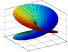
Figure 3: To make the complex function one-to-one, one needs to extend the complex plane to the two-fold cover called the two-fold Riemann Surface.

Suppose we want to compute $\mathbf{d}_{\mathrm{N}}(x,y)$ where $P=\{(0,0)\}$. Writing $(x,y)\in\mathbb{C}$ in polar coordinates as $z=re^{i\theta}$, we define the quadratic transformation $f\colon\mathbb{C}\to\mathcal{R}$ by

$$f(z)=z^{2}/2=(r^{2}/2)e^{i2\theta},$$

where $\mathcal{R}$ is the two-fold Riemann surface; see Figure 3. The important point here is that the image is a double covering of $\mathbb{C}$. For example, the points $1$ and $-1$ are mapped to different copies of $1/2$. Therefore, on the Riemann surface, the distance between $1$ and $-1$ is one and the shortest path goes through the origin. More generally, given any two nonzero points $p$ and $q$ on the surface, the minimum angle between them (measured with respect to the origin) will be between 0 and $2\pi$. Moreover, if this angle is $\geq\pi$, then the shortest path between them will consist of the two straight lines $[p,0]$ and $[0,q]$. Otherwise, the line $[p,q]$ will be a line on the surface and, thus, the geodesic from $p$ to $q$.

Let $\mathbf{d}_{\mathcal{R}}$ denote the distance on the Riemann surface. We next show that for a single point, the nearest neighbor geodesic is identical to the geodesic on the Riemann surface.

Lemma 5.1.

Let $\gamma\colon[0,1]\to\mathbb{C}$ be a curve. Then, the image of $\gamma$ under $f$, denoted by $f\circ\gamma$ satisfies the following property:

$$\mathbf{d}_{\mathcal{R}}(f\circ\gamma)=\mathbf{\ell}_{\mathrm{N}}(\gamma).$$

Proof.

Suppose $\gamma\colon[0,1]\to\mathbb{C}$ is any piecewise differentiable curve, and let $\alpha:=f\circ\gamma$. The $\mathrm{N}$-length $\mathbf{\ell}_{\mathrm{N}}(\gamma)$ of $\gamma$ is the finite sum of the $\mathrm{N}$-length of all differentiable pieces of $\gamma$. If the path $\gamma$ goes through the origin, we further break the path at the origin so that $\alpha$ is also differentiable. Thus, it suffices to consider $(a,b)\subset[0,1]$ so that $\gamma[a,b]$ is a differentiable piece of $\gamma$. Then, we have

$$\mathbf{\ell}_{\mathrm{N}}(\gamma[a,b]) =\int_{a}^{b}|\gamma(t)||\gamma^{\prime}(t)|\,dt |\cdot|$$ is modulus.

$$=\int_{a}^{b}|\gamma(t)\gamma^{\prime}(t)|\,dt$$ Modulus commutes with product.

$$=\int_{a}^{b}|\alpha^{\prime}(t)|\,dt$$ Chain rule.

$$=\mathbf{\ell}_{\mathcal{R}}(\alpha[f(a),f(b)]).$$

∎

Corollary 1 (Reduction to Euclidean Distances on a Riemann Surface).

Given three points $x$, $y$, and $p$ in $\mathbb{R}^{d}$ such that $p=\mathop{\mathrm{NN}}(x)=\mathop{\mathrm{NN}}(y)$, the nearest neighbor geodesic $G$ from $x$ to $y$ satisfies the following properties:

1. $G$ is in the plane determined by $x,y,p$.

2. 1. If the angle formed by $x,p,y$ is $\pi/2$ or more, then $G$ consists of the two straight segments $\overline{xp}$ and $\overline{py}$.

   2. Otherwise, $G$ is the preimage of the straight line from $f(x)$ to $f(y)$, where $f$ is the quadratic map in the plane given by $x,y,p$ to the Riemann Surface.

5.2 Discretizing a Path

First we approximate any $(x,y)$-path $\gamma$ with a piecewise linear $(x,y)$-path $\alpha$ that is composed of segments that are sufficiently long. The properties of $\alpha$, formalized in the following definition, are used in the rest of this section to obtain a piecewise linear approximation using Steiner points.

Definition 5.1.

Let $P=\{p_{1},p_{2},\cdots,p_{n}\}$ be a set of points in $\mathbb{R}^{d}$, and let $x,y\in P$. Assume $\gamma$ is a path from $x$ to $y$ that is internally disjoint from $P$. Also, let $0<\varepsilon_{\alpha}<1$ be a real number. A sequence $\{0=t_{0},t_{1},\dots,t_{k},t_{k+1}=1\}$ is a $\varepsilon_{\alpha}$-discretizing sequence of $\gamma$ if it has the following properties:

1. The nearest neighbor of both $\gamma(t_{1})$ and $\gamma(t_{2})$ is $x$, while the nearest neighbor of both $\gamma(t_{k-1})$ and $\gamma(t_{k})$ is $y$.

2. For all $1\leq i\leq k$, we have $\mathbf{d}(\gamma(t_{i}),\gamma(t_{i+1}))=\varepsilon_{\alpha}\cdot\mathrm{N}(\gamma(t_{i}))$.

In this case, the piecewise linear path $\alpha=\{x,\gamma(t_{1}),\dots,\gamma(t_{k}),y\}$ is a $\varepsilon_{\alpha}$-discretized path of $\gamma$.

The following lemma guarantees the existence of $\varepsilon_{\alpha}$-discretizing sequences and, hence, $\varepsilon_{\alpha}$-discretized paths. Its proof is essentially the same as the proof of Lemma 4.2.

Lemma 5.2.

Let $P=\{p_{1},p_{2},\cdots,p_{n}\}$ be a set of points in $\mathbb{R}^{d}$, and let $x,y\in P$. Let $\gamma$ be a path from $x$ to $y$ that is internally disjoint from $P$ and $0<\varepsilon_{\alpha}<1$ a real number. There exists a $\varepsilon_{\alpha}$-discretizing sequence of $\gamma$.

Next, we show that the $\mathrm{N}$-length of a $\varepsilon_{\alpha}$-discretized path of $\gamma$ is not much longer than the $\mathrm{N}$-length of $\gamma$.

Lemma 5.3.

If $\alpha$ is a $\varepsilon_{\alpha}$-discretized path of $\gamma$ for some $\varepsilon_{\alpha}\leq 1/2$, then $\mathbf{\ell}_{\mathrm{N}}(\alpha)\leq(1+4\varepsilon_{\alpha})\mathbf{\ell}_{\mathrm{N}}(\gamma)$.

Proof.

For $1\leq i\leq k-1$, let $\alpha_{i}$ be the line segment $(\gamma(t_{i}),\gamma(t_{i+1}))$. Furthermore, let $\alpha_{0}$ and $\alpha_{k}$ be the line segments $(x,\gamma(t_{1}))$ and $(\gamma(t_{k}),y)$, respectively. Also, let $\gamma_{i}=\gamma[t_{i},t_{i+1}]$, for $1\leq i\leq k-1$, and $\gamma_{0}=\gamma[0,t_{1}]$ and $\gamma_{k}=\gamma[t_{k},1]$.

We prove the stronger statement that $\mathbf{\ell}_{\mathrm{N}}(\alpha_{i})\leq(1+4\varepsilon_{\alpha})\mathbf{\ell}_{\mathrm{N}}(\gamma_{i})$, for any $0\leq i\leq k$. For $i\in\{0,k\}$, the straight line is indeed the shortest path in the nearest neighbor metric (since $\mathrm{N}(\gamma(t_{1}))=\gamma(t_{0})=x$ and $\mathrm{N}(\gamma(t_{k}))=\gamma(t_{k+1})=y$), and so, $\mathbf{\ell}_{\mathrm{N}}(\alpha_{i})\leq\mathbf{\ell}_{\mathrm{N}}(\gamma_{i})$. For $1\leq i\leq k-1$, by Lemma 5.4,

$$\mathbf{\ell}_{\mathrm{N}}(\alpha_{i})\leq\mathbf{\ell}_{\mathrm{N}}(\gamma_{i})\cdot\frac{\mathrm{N}(\gamma(t_{i}))+\mathbf{\ell}(\alpha_{i})}{\mathrm{N}(\gamma(t_{i}))-\mathbf{\ell}(\alpha_{i})}.$$

Then, by the second property of $\varepsilon_{\alpha}$-discretizing sequences,

$$\mathbf{\ell}_{\mathrm{N}}(\alpha_{i})\leq\mathbf{\ell}_{\mathrm{N}}(\gamma_{i})\cdot\frac{\mathrm{N}(\gamma(t_{i}))+\varepsilon_{\alpha}\mathrm{N}(\gamma(t_{i}))}{\mathrm{N}(\gamma(t_{i}))-\varepsilon_{\alpha}\mathrm{N}(\gamma(t_{i}))}.$$

After simplifying and using the fact that $\varepsilon_{\alpha}\leq 1/2$, we obtain

$$\mathbf{\ell}_{\mathrm{N}}(\alpha_{i})\leq\mathbf{\ell}_{\mathrm{N}}(\gamma_{i})\cdot\frac{1+\varepsilon_{\alpha}}{1-\varepsilon_{\alpha}}\leq\mathbf{\ell}_{\mathrm{N}}(\gamma_{i})\cdot(1+4\varepsilon_{\alpha}).$$

∎

5.3 Approximating with Steiner Points

Assume $P\subset\mathbb{R}^{d}$, $x,y\in P$, and let $\gamma$ be an arbitrary $(x,y)$-path. We show how to approximate $\gamma$ with a piecewise linear path through a collection of Steiner points in $\mathbb{R}^{d}$. To obtain an accurate estimation of $\gamma$, we require the Steiner points to be sufficiently dense. The following definition formalizes this density with a parameter $\delta$.

Definition 5.2 ($\delta$-sample).

Let $P=\{p_{1},p_{2},\cdots,p_{n}\}$ be a set of points in $\mathbb{R}^{d}$, and let $D\subseteq\mathbb{R}^{d}$. For a real number $0<\delta<1$, a $\delta$-sample is a (possibly infinite) set of points $T\subseteq D$ such that if $z\in D\setminus P$, then $\mathbf{d}(z,T)\leq\delta\cdot\mathrm{N}(z)$.

The following lemmas guarantees that an accurate estimation of $\gamma$ can be computed using a $\delta$-sample.

Lemma 5.4.

Let $P=\{p_{1},p_{2},\cdots,p_{n}\}$ be a set of points in $\mathbb{R}^{d}$, and let $x,y\in\mathbb{R}^{d}$. Let $\gamma$ be any path from $x$ to $y$, and $l$ be the straight $(x,y)$-segment. Assume further that $\mathrm{N}(x)>\mathbf{\ell}(l)$. Then,

$$\mathbf{\ell}_{\mathrm{N}}(l)\leq\mathbf{\ell}_{\mathrm{N}}(\gamma)\cdot\frac{\mathrm{N}(x)+\mathbf{\ell}(l)}{\mathrm{N}(x)-\mathbf{\ell}(l)}$$

Proof.

Let $\gamma^{\prime}=\gamma\cap B(x,\mathbf{\ell}(l))$. Observe that $\gamma^{\prime}$ is a finite collection paths, and let $\mathbf{\ell}(\gamma^{\prime})$ be the total length of these paths.

Figure 4: Proof of Lemma 5.4; $\gamma^{\prime}$ is bold.

For any point $z\in B(x,\mathbf{\ell}(l))$ we have $\mathrm{N}(x)-\mathbf{\ell}(l)\leq\mathrm{N}(z)\leq\mathrm{N}(x)+\mathbf{\ell}(l)$ because $\mathrm{N}(\cdot)$ is Lipschitz. Since $\gamma^{\prime}$ and $l$ are both contained in $B(x,\mathbf{\ell}(l))$, in particular, we have:

$$\mathbf{\ell}_{\mathrm{N}}(\gamma^{\prime})\geq\mathbf{\ell}(\gamma^{\prime})(\mathrm{N}(x)-\mathbf{\ell}(l))$$

and

$$\mathbf{\ell}_{\mathrm{N}}(l)\leq\mathbf{\ell}(l)(\mathrm{N}(x)+\mathbf{\ell}(l))\leq\mathbf{\ell}(\gamma^{\prime})(\mathrm{N}(x)+\mathbf{\ell}(l)).$$

Thus, since $\gamma^{\prime}\subseteq\gamma$, we have $\mathbf{\ell}_{\mathrm{N}}(\gamma^{\prime})\leq\mathbf{\ell}_{\mathrm{N}}(\gamma)$. Finally, because both sides of the inequalities are positive numbers, we have:

$$\frac{\mathbf{\ell}_{\mathrm{N}}(l)}{\mathbf{\ell}_{\mathrm{N}}(\gamma)}\leq\frac{\mathbf{\ell}_{\mathrm{N}}(l)}{\mathbf{\ell}_{\mathrm{N}}(\gamma^{\prime})}\leq\frac{\mathrm{N}(x)+\mathbf{\ell}(l)}{\mathrm{N}(x)-\mathbf{\ell}(l)}.$$

∎

Lemma 5.5.

Let $P=\{p_{1},p_{2},\cdots,p_{n}\}$ be a set of points in $\mathbb{R}^{d}$, and let $S$ be a $\delta$-sample, and let $0<\delta<1/10$. Then, for any pair of points $x,y\in P$, there is a piecewise linear path $\eta=(x,s_{1},\dots,s_{k},y)$, where $s_{1},\dots,s_{k}\in S$, such that:

$$\mathbf{\ell}_{\mathrm{N}}(\eta)\leq(1+C_{1}\delta^{2/3})\mathbf{d}_{\mathrm{N}}(x,y),$$

and, for all $1\leq i\leq k-1$,

$$\mathbf{\ell}_{\mathrm{N}}((s_{i},s_{i+1}))\leq C_{2}\cdot\delta^{2/3}\cdot\mathrm{N}(s_{i}).$$

$C_{1}$ and $C_{2}$ are universal constants.

Proof.

Let $\gamma$ be an $(x,y)$-shortest path under the nearest neighbor metric. We assume, without loss of generality, that $\gamma$ is internally disjoint from $P$. Of course, we can break any path to such pieces and use induction to prove the lemma for the general case.

Let $\alpha=(x=\gamma(t_{0}),\gamma(t_{1}),\dots,\gamma(t_{k+1})=y)$ be a $(2\delta^{2/3})$-discretization of $\gamma$. For all $0\leq i\leq k$, let $\alpha_{i}=(\gamma(t_{i}),\gamma(t_{i+1}))$ for $0\leq i\leq k$, let $m_{i}$ be the midpoint of $\alpha_{i}$, and let $s_{i}\in S$ be the closest Steiner point to $m_{i}$. Then, let $\beta_{i}=(\gamma(t_{i}),s_{i},\gamma(t_{i+1}))$ be a two-segment path, and let $\beta=\beta_{0}\circ\beta_{1}\circ\dots\circ\beta_{k}$. Finally, let $\eta=(x,s_{1},s_{2},\dots,s_{k-1},y)$, and let $\eta_{i}=(s_{i},s_{i+1})$ where $0\leq i<k$ and $s_{0}=x$ and $s_{k}=y$ to simplify notation.

We need to prove that $\mathbf{\ell}_{\mathrm{N}}(\eta)\leq(1+C_{1}\delta^{2/3})\mathbf{\ell}_{\mathrm{N}}(\gamma)$. Lemma 5.3 implies that

$$\mathbf{\ell}_{\mathrm{N}}(\alpha)\leq(1+8\delta^{2/3})\mathbf{\ell}_{\mathrm{N}}(\gamma)$$

Showing the following two facts imply the statement of the lemma.

$$\mathbf{\ell}_{\mathrm{N}}(\beta)\leq(1+20\delta^{2/3})\mathbf{\ell}_{\mathrm{N}}(\alpha)$$ (5)

$$\mathbf{\ell}_{\mathrm{N}}(\eta)\leq(1+8\delta^{2/3})\mathbf{\ell}_{\mathrm{N}}(\beta)$$ (6)

Figure 5: The lines segment $\alpha_{i}$ is blue, and the two-segment path $\beta_{i}$ is red.

A proof of Inequality (5):

We prove the stronger statement that for all $0\leq i\leq k$, $\mathbf{\ell}_{\mathrm{N}}(\beta_{i})\leq(1+8\delta^{2/3})\mathbf{\ell}_{\mathrm{N}}(\alpha_{i})$. Recall that $m_{i}$ is the midpoint of $\alpha_{i}$ and $s_{i}\in S$ is the closest Steiner point to $m_{i}$. Let $h_{i}$ be the closes point of $\alpha_{i}$ to $s_{i}$; see Figure 5.

Because $\mathbf{\ell}(\alpha_{i})\approx\delta^{2/3}\;\mathrm{N}(m_{i})$, $\mathbf{\ell}((m_{i},s_{i}))\approx\delta\;\mathrm{N}(m_{i})$, and $\delta\leq\delta^{2/3}$, we have $(s_{i},h_{i})$ is orthogonal to $\alpha_{i}$. Then, the following bound on the length of the piecewise linear path $\beta_{i}=(\gamma(t_{i}),s_{i},\gamma(t_{i+1}))$ is implied by the Pythagorean theorem using derivative to maximize a function.

$$\mathbf{\ell}(\beta_{i})\leq 2\cdot\sqrt{\left(\frac{\mathbf{\ell}(\alpha_{i})}{2}\right)^{2}+(\mathbf{\ell}(s_{i},h_{i}))^{2}}\leq 2\cdot\sqrt{\left({\delta^{2/3}\mathrm{N}(\gamma(t_{i}))}\right)^{2}+\left(\delta\mathrm{N}(m_{i})\right)^{2}}$$ (7)

Then, the Lipschitz property of the $\mathrm{N}$-function implies:

$$\mathrm{N}(m_{i})\leq\mathrm{N}(\gamma(t_{i}))+\frac{\mathbf{\ell}(\alpha_{i})}{2}\leq\mathrm{N}(\gamma(t_{i}))+{\delta^{2/3}\cdot\mathrm{N}(\gamma(t_{i}))}\leq(1+\delta^{2/3})\mathrm{N}(\gamma(t_{i})).$$

By substituting $(1+\delta^{2/3})\mathrm{N}(\gamma(t_{i}))$ for $\mathrm{N}(m_{i})$ in (7), we obtain

$$\mathbf{\ell}(\beta_{i}) \leq 2\cdot\sqrt{\left({\delta^{2/3}\mathrm{N}(\gamma(t_{i}))}\right)^{2}+\left(\delta(1+\delta^{2/3})\mathrm{N}(\gamma(t_{i}))\right)^{2}}$$

$$= \delta^{2/3}\mathrm{N}(\gamma(t_{i}))\cdot\sqrt{1+\left({\delta^{1/3}(1+\delta^{2/3})}\right)^{2}}$$

$$= \mathbf{\ell}(\alpha_{i})\cdot\left(1+2\delta^{2/3}\right)$$

On the other hand, because both $\alpha_{i}$ and $\beta_{i}$ are contained in $B(\gamma(t_{i}),\varepsilon_{\alpha}\mathrm{N}(\gamma(t_{i})))$, for any point $z\in\alpha_{i}\cup\beta_{i}$ we have $\mathrm{N}(\gamma(t_{i}))(1-2\delta^{2/3})\leq\mathrm{N}(z)\leq\mathrm{N}(\gamma(t_{i}))(1+2\delta^{2/3})$ and so

$$\mathbf{\ell}_{\mathrm{N}}(\beta_{i})\leq\mathbf{\ell}(\beta_{i})\cdot\mathrm{N}(\gamma(t_{i}))(1+2\delta^{2/3}).$$

and

$$\mathbf{\ell}_{\mathrm{N}}(\alpha_{i})\geq\mathbf{\ell}(\alpha_{i})\cdot\mathrm{N}(\gamma(t_{i}))(1-2\delta^{2/3}).$$

Last three inequalities together imply

$$\frac{\mathbf{\ell}_{\mathrm{N}}(\beta_{i})}{\mathbf{\ell}_{\mathrm{N}}(\alpha_{i})} \leq \frac{1+2\delta^{2/3}}{1-2\delta^{2/3}}\cdot\left(1+2\delta^{2/3}\right)$$

$$\leq (1+20\delta^{2/3}).$$

Thus, we obtain Inequality (5) by summing over all $\alpha_{i}$’s and $\beta_{i}$’s.

A proof of Inequality (6):

First, by the triangle inequality, we obtain:

$$\mathbf{\ell}(\eta_{i}) \leq \mathbf{\ell}(s_{i},t_{i+1})+\mathbf{\ell}(t_{i+1},s_{i+1})$$

$$= 2\delta^{2/3}\cdot\left(\frac{\mathrm{N}(\gamma(t_{i}))+\mathrm{N}(\gamma(t_{i+1}))}{2}\right)$$

$$\leq 2\delta^{2/3}\cdot\max\left(\mathrm{N}(\gamma(t_{i})),\mathrm{N}(\gamma(t_{i+1}))\right)$$

Then, Lemma 5.4, letting $x$ be the endpoint with larger $\mathrm{N}$ value, implies

$$\mathbf{\ell}_{\mathrm{N}}(\eta_{i})\leq\mathbf{\ell}_{\mathrm{N}}(s_{i},t_{i+1},s_{i+1})\cdot\frac{1+2\delta^{2/3}}{1-2\delta^{2/3}}\leq\mathbf{\ell}_{\mathrm{N}}(s_{i},t_{i+1},s_{i+1})\cdot(1+8\delta^{2/3}).$$

Finally, by summing over all $\eta_{i}$’s we obtain Inequality 6, and the proof is complete. ∎

5.4 The Approximation Graph

So far we have shown that any shortest path can be approximated using a $\delta$-sample that is composed of infinitely many points. In addition, we know how to compute the exact $\mathrm{N}$-distance between any pair of points if they reside in the same Voronoi cell of $\mathrm{Vor}(P)$. Here, we combine these two ideas to be able to approximate any shortest path using only a finite number of Steiner points. The high-level idea is to use the Steiner point approximation while $\gamma$ passes through regions that are far from $P$ and switch to the exact distance computation as soon as $\gamma$ is sufficiently close to one of the points in $P$.

Let $P=\{p_{1},p_{2},\cdots,p_{n}\}$ be a set of points in $\mathbb{R}^{d}$, and let $B$ be any convex body that contains $P$. Fix $\delta\in(0,1)$, and for any $1\leq i\leq n$, let $r_{i}=r_{P}(p_{i})$ be the inradius of the Voronoi cell with site $p_{i}$. Also, let $u_{i}=(1-\delta^{2/3})r_{i}$. Finally, let $S$ be a $\delta$-sample on the domain $B\setminus{\bigcup_{1\leq i\leq n}{B(p_{i},u_{i})}}$.

Definition 5.3 (Approximation Graph).

The approximation graph $\mathcal{A}=\mathcal{A}(P,\{u_{1},\dots,u_{n}\},S,\delta)=(V_{\mathcal{A}},E_{\mathcal{A}})$ is a weighted undirected graph, with weight function $w:E_{\mathcal{A}}\rightarrow\mathbb{R}^{+}$. The vertices in $V_{\mathcal{A}}$ are in one to one correspondence with the points in $S\cup P$; for simplicity we use the same notation to refer to corresponding elements in $S\cup P$ and $V_{\mathcal{A}}$. The set $E_{\mathcal{A}}$ is composed of three types of edges:

1. If $s_{1},s_{2}\in S$ and $s_{1},s_{2}\in B(p_{i},r_{i})$ for any $p_{i}$, then $(s_{1},s_{2})\in E_{\mathcal{A}}$ and $w(s_{1},s_{2})=\mathbf{d}_{\mathrm{N}}(s_{1},s_{2})$. We compute this distance using Corollary 1.

2. Otherwise, if $s_{1},s_{2}\in S$ and $\mathbf{\ell}(s_{1},s_{2})\leq C_{2}\delta^{2/3}\max(\mathrm{N}(s_{1}),\mathrm{N}(s_{2}))$, where $C_{2}$ is the constant of Lemma 5.5, then $(s_{1},s_{2})\in E_{\mathcal{A}}$ and $w(s_{1},s_{2})=\max(\mathrm{N}(s_{1}),\mathrm{N}(s_{2}))\cdot\mathbf{\ell}(s_{1},s_{2})$.

3. If $s_{1}\in S$ and $s_{1}\in B(p_{i},r_{i})$ then $(p_{i},s_{1})\in E_{\mathcal{A}}$ and $w(p_{i},s_{1})=\mathbf{d}_{\mathrm{N}}(p_{i},s_{1})=(\mathbf{d}(p_{i},s_{1}))^{2}/2$; see Corollary 1.

For $x,y\in V_{\mathcal{A}}$ let $\mathbf{d}_{\mathcal{A}}(x,y)$ denote the length of the shortest path from $x$ to $y$ in the graph $\mathcal{A}$.

The following lemma guarantees that the shortest paths in the approximation graph are sufficiently accurate estimations.

Lemma 5.6.

Let $\{u_{1},\dots,u_{n}\}$, $S$ and $\delta$ be defined as above. Let $\mathcal{A}(P,\{u_{1},\dots,u_{n}\},S,\delta)$ be the approximation graph for $P$. For any pair of points $x,y\in P$ we have:

$$(1-C_{2}\delta^{2/3})\cdot\mathbf{d}_{\mathrm{N}}(x,y)\leq\mathbf{d}_{\mathcal{A}}(x,y)\leq(1+C_{4}\delta^{2/3})\cdot\mathbf{d}_{\mathrm{N}}(x,y),$$

where $C_{2}$ and $C_{4}$ are constants computable in $O(1)$ time.

Proof.

First, we prove the upper bound. Let $D=B\setminus{\bigcup_{1\leq i\leq n}{B(p_{i},u_{i})}}$, and recall that $S$ is a $\delta$-sample on $D$. Let $S^{+}$ be a $\delta$-sample of $B$ such that $S^{+}\cap D=S$. According to Lemma 5.5, there is a piecewise linear path $\eta=\{x,s_{1},\dots,s_{k},y\}$, for $s_{1},\dots,s_{k}\in S^{+}$, such that $\mathbf{\ell}_{\mathrm{N}}(\eta)\leq(1+C_{1}\delta^{2/3})\mathbf{d}_{\mathrm{N}}(x,y)$. We use $\eta$ to obtain a $(x,y)$-path $\sigma$ in $\mathcal{A}$ with length at most $(1+2C_{2}\delta^{2/3})\mathbf{\ell}_{\mathrm{N}}(\eta)$; $C_{2}$ is the constant in Lemma 5.5.

Consider any maximal subpath $\eta^{\prime}=(s_{i},s_{i+1},\dots,s_{j-1},s_{j})$ of $\eta$ that resides in $B\left(p_{t},u_{t}/(1-\delta^{2/3})\right)$ for a $p_{t}\in P$. The lengths of the type (2) edges and the second inequality of Lemma 5.5 imply that $s_{i},s_{j}\notin B(p_{t},u_{t})$, which in turn implies that $s_{i},s_{j}\in D$. Further, $(s_{i},s_{j})$ is a type (1) edge of $\mathcal{A}$ and $w(s_{i},s_{j})=\mathbf{\ell}_{\mathrm{N}}(s_{i},s_{j})\leq\mathbf{\ell}_{\mathrm{N}}(\eta^{\prime})$. So, $\eta^{\prime}$ in $\eta$ corresponds to a single type (1) edge $(s_{i},s_{j})$ in $\sigma$ with no longer length. In fact, all type (1) edges of $\sigma$ correspond to not shorter paths in $\eta$.

Similarly, we consider maximal paths $(p,s_{i},s_{i+1},\dots,s_{j-1},s_{j})$, where $p$ is an input point, and replacing them with type (3) edges of $\sigma$. Again, all type (3) edges of $\sigma$ correspond to not shorter paths of $\eta$.

It remains to show that type (2) edges of $\sigma$ are not too long. Observe, that each type (2) edge of $\sigma$ corresponds to a line segment of $\eta$. Let $(s_{1},s_{2})\in E_{\mathcal{A}}$ be a type (2) edge and let $\max(\mathrm{N}(s_{1}),\mathrm{N}(s_{2}))=\mathrm{N}(s_{1})$ without loss of generality. By the Lipschitz property and the length property of type (2) edges

$$\mathbf{\ell}_{\mathrm{N}}(s_{1},s_{2})\geq(\mathrm{N}(s_{1})-\mathbf{\ell}(s_{1},s_{2}))\mathbf{\ell}(s_{1},s_{2})\geq(1-C_{2}\delta^{2/3})\mathrm{N}(s_{1})\mathbf{\ell}(s_{1},s_{2})=(1-C_{2}\delta^{2/3})w(s_{1},s_{2}),$$

which implies

$$w(s_{1},s_{2})\leq(1+2C_{2}\delta^{2/3})\mathbf{\ell}_{\mathrm{N}}(s_{1},s_{2}),$$

and so, by Lemma 5.5,

$$\mathbf{\ell}_{\mathcal{A}}(\sigma)\leq(1+2C_{2}\delta^{2/3})\mathbf{\ell}_{\mathrm{N}}(\eta)\leq(1+C_{4}\delta^{2/3})\mathbf{d}_{\mathrm{N}}(x,y).$$

To prove the lower bound, let $x,y\in V_{\mathcal{A}}$ and let $\sigma=(x,s_{1},\dots,s_{k},y)$ be a path from $x$ to $y$ in $\mathcal{A}$. Also, let $\gamma$ be the $(x,y)$ path in $\mathbb{R}^{d}$ that hits $(x=s_{0},s_{1},\dots,s_{k},y=s_{k+1})$ in this order, and let the $(s_{i},s_{j})$ subpath of $\gamma$ be a line segment if $(s_{i},s_{j})$ is a type (2) edge in $\mathcal{A}$ and be the shortest $(s_{i},s_{j})$ nearest neighbor path otherwise. Then, let $\gamma_{i}$ be the subpath of $\gamma$ from $s_{i}$ to $s_{i+1}$. We compare $w(s_{i},s_{i+1})$ with $\mathbf{\ell}_{\mathrm{N}}(\gamma_{i})$.

If $(s_{i},s_{i+1})$ is type (1) or (3) then $\mathbf{\ell}_{\mathrm{N}}(\gamma_{i})=w(s_{1},s_{2})$. Otherwise, $(s_{i},s_{i+1})$ is type (2) and by Lipschitz property

$$\mathbf{\ell}_{\mathrm{N}}(s_{1},s_{2})\leq(\mathrm{N}(s_{1})+\mathbf{\ell}(s_{1},s_{2}))\mathbf{\ell}(s_{1},s_{2})\leq(1+C_{2}\delta^{2/3})\mathrm{N}(s_{1})\mathbf{\ell}(s_{1},s_{2})=(1+C_{2}\delta^{2/3})w(s_{1},s_{2}).$$

Overall,

$$\mathbf{d}_{\mathrm{N}}(x,y)\leq\mathbf{\ell}_{\mathrm{N}}(\gamma)\leq(1+C_{2}\delta^{2/3})\mathbf{\ell}_{\mathcal{A}}(\sigma),$$

and the proof is complete. ∎

5.5 Construction of Steiner Points

The only remaining piece that we need to obtain an approximation scheme is an algorithm for computing a $\delta$-sample. For this section, given a point set $T$ and $x\in T$, let $r_{T}(x)$ denote the inradius of the Voronoi cell of $\mathrm{Vor}(T)$ that contains $x$. Also, given a set $T$ and an arbitrary point $x$ (not necessarily in $T$), let $\mathbf{f}_{T}(x)$ denote the distance from $x$ to its second nearest neighbor in $T$.

We can apply existing algorithms for generating meshes and well-spaced points to compute a $\delta$-sample on $\mathcal{D}\setminus\bigcup_{i}B(p_{i},u_{i})$, where $\mathcal{D}\subseteq\mathbb{R}^{d}$ is a domain, and $u_{i}=(1-\delta^{2/3})r_{P}(p_{i})$. The procedure consists of two steps:

1. Use the algorithm of [MSV13] to construct a well-spaced point set $M$ (along with its associated approximate Delaunay graph) with aspect ratio $\tau$ in time $2^{O(d)}(n\log n+|M|)$.

2. Then over-refine $M$ to $S$ for the sizing function $g(x)=\frac{2\delta}{11\tau}\mathbf{f}_{P}(x)$ (while maintaining aspect ratio $\tau$) in time $2^{O(d)}|S|$ by using the algorithm of Section 3.7 in [She11]. (see also [HOMS10] for an earlier use of this technique)

In the above algorithm, we will choose $\tau$ to be a fixed constant, say, $\tau=6$. Both of the meshing algorithms listed above are chosen for their theoretical guarantees on running time. In practice, one could use any quality Delaunay meshing algorithm, popular choices include Triangle [She96] in $\mathbb{R}^{2}$ and Tetgen [Si11] or CGAL [ART⁺12] in $\mathbb{R}^{3}$.

From the guarantees in ([She11]), we know that

$$|S|=O\left(\int_{\mathcal{D}}\frac{dx}{g(x)^{d}}\right)=\delta^{-O(d)}n\log\Delta,$$ (8)

where $\Delta$ is the spread of $P$, i.e., the ratio of the largest distance between two points in $P$ to the smallest distance between two points in $P$.

Lemma 5.7.

If $x\in\mathcal{D}\setminus B(p_{i},u_{i})$, where $p_{i}=\mathop{\mathrm{NN}}(x)$, then $\mathrm{N}(x)\leq f_{P}(x)\leq 5\mathrm{N}(x)$.

Proof.

Note that $N(x)\leq f_{P}(x)$ is trivial. To prove the second half of the inequality, let $q$ be the closest point to $p$ in $P\setminus\{p_{i}\}$. Then, by the triangle inequality, we have that

$$f_{P}(x) \leq \mathbf{d}(x,q)$$

$$\leq \mathbf{d}(x,p_{i})+\mathbf{d}(p_{i},q)$$

$$\leq \mathbf{d}(x,p_{i})+2r_{P}(p_{i})$$

$$\leq \mathbf{d}(x,p_{i})+\frac{2}{1-\delta^{2/3}}\mathbf{d}(x,p_{i})$$

$$= 5\mathbf{d}(x,p_{i})$$

$$= 5\mathrm{N}(x).$$

∎

Now, it remains to show that the point set $S$ is indeed a $\delta$-sample on $\mathcal{D}\setminus\bigcup_{i}B(p_{i},u_{i})$. This is provided by the following lemma.

Lemma 5.8.

$S$ is a $\delta$-sample on $\mathcal{D}\setminus\bigcup_{i}B(p_{i},u_{i})$.

Proof.

Let $x\in\mathcal{D}\setminus\bigcup_{i}B(p_{i},u_{i})$ be an arbitrary point. Then, let $q$ be the closest point to $x$ that lies in $S$. Note that

$$\mathbf{d}(x,q) \leq \tau\cdot r_{S}(q)$$

$$\leq \tau\left(\frac{2\delta}{11\tau}\mathbf{f}_{P}(q)\right)$$

$$\leq \frac{2\delta}{11}(\mathbf{f}_{P}(x)+\mathbf{d}(x,q)).$$

This implies that

$$\mathbf{d}(x,q) \leq \frac{2\delta}{11-2\delta}\mathbf{f}_{P}(x)$$

$$\leq \frac{10\delta}{11-2\delta}\mathrm{N}(x)$$

$$\leq \delta\mathrm{N}(x),$$

as desired. ∎

Now, we calculate the number of edges that will be present in the approximation graph defined in the previous section. For this, we require a few lemmas.

Lemma 5.9.

Let $A=B(p_{i},r_{P}(p_{i}))\setminus B(p_{i},u_{i})$ be an annulus around $p_{i}$. Then, $|A\cap S|=\delta^{-O(d)}$.

Proof.

By the meshing guarantees of [She11], we know that for any point $s\in A\cap S$, $B(s,t)$ does not contain a point from $S\setminus\{s\}$ for $t=\Omega(r_{S}(s))=\Omega(\delta\cdot r_{P}(p))$. Thus, the desired result follows using a simple sphere packing argument. ∎

Lemma 5.10.

If $s\in S$, then $|B(s,C_{2}\delta^{2/3}\mathrm{N}(s))\cap S|=\delta^{-O(d)}$, where $C_{2}$ is the constant in Lemma 5.5.

Proof.

As in the previous lemma, meshing guarantees tell us that for any $s^{\prime}\in B(s,C_{2}\delta^{2/3}\mathrm{N}(s))$, we have that $B(s^{\prime},t)$ does not contain a point from $S\setminus\{s^{\prime}\}$ for $t=\Omega(\delta\cdot\mathrm{N}(s^{\prime}))=\Omega(\delta\cdot\mathrm{N}(s))$. Thus, we again obtain the desired result from a sphere packing argument. ∎

From the above lemmas, we see that $\mathcal{A}$ is composed of $|S|=\delta^{-O(d)}n\log\Delta$ vertices and $n\delta^{-O(d)}+|S|\cdot\delta^{-O(d)}=|S|\cdot\delta^{-O(d)}$ edges.

Remark. Note that the right hand side of (8) is in terms of the spread, a non-combinatorial quantity. Indeed, one can construct examples of $P$ for which the integral in (8) is not bounded from above by any function of $n$. However, for many classes of inputs, one can obtain a tighter analysis. In particular, if $P$ satisfies a property known as well-paced, one can show that the resulting set $S$ will satisfy $|S|=2^{O(d)}n$ (see [MPS08, She12]).

In a more general setting (without requiring that $P$ is well-paced), one can modify the algorithms to produce output in the form of a hierarchical mesh [MPS11]. This then produces an output of size $2^{O(d)}n$, and $(1+\varepsilon)$-approximation algorithm for the nearest neighbor metric can be suitably modified so that the underlying approximation graph uses a hierarchical set of points instead of a full $\delta$-sample. However, we ignore the details here for the sake of simplicity of exposition.

The above remark, along with the edge count of $\mathcal{A}$ and the running time guarantees from [MSV13], yields Theorem 1.2, the main theorem of this section.

6 Discussion

Motivated by estimating geodesic distances within subsets of $\mathbb{R}^{n}$, we consider two distance metrics in this paper: the $N$-distance and the edge-squared distance. The main focus of this paper is to find an approximation of the $N$-distance. One possible drawback of our $(1+\varepsilon)$-approximation algorithm is its exponential dependency on $d$. To alleviate this dependency a natural approach is using a Johnson-Lindenstrauss type projection. Thereby, we would like to ask which properties are preserved under random projections such as those in Johnson-Lindenstrauss transforms.

We are currently working on implementing the approximation algorithm presented in Section 4. We hope to show that this approximation is fast in practice as well as in theory.

References

- [AG95] Helmut Alt and Michael Godau. Computing the Fréchet distance between two polygonal curves. International Journal of Computational Geometry & Applications, 5(01n02):75–91, 1995.
- [ALMS98] Lyudmil Aleksandrov, Mark Lanthier, Anil Maheshwari, and Jörg-Rüdiger Sack. An epsilon-approximation for weighted shortest paths on polyhedral surfaces. In 6th WS on Algorithm Theory, pages 11–22, London, UK, UK, 1998.
- [AMS00] Lyudmil Aleksandrov, Anil Maheshwari, and Jörg-Rüdiger Sack. Approximation algorithms for geometric shortest path problems. In Proceedings of the thirty-second annual ACM symposium on Theory of computing, STOC ’00, pages 286–295, New York, NY, USA, 2000. ACM.
- [AMS05] L. Aleksandrov, A. Maheshwari, and J.-R. Sack. Determining approximate shortest paths on weighted polyhedral surfaces. J. ACM, 52(1):25–53, January 2005.
- [ART+12] Pierre Alliez, Laurent Rineau, Stéphane Tayeb, Jane Tournois, and Mariette Yvinec. 3D mesh generation. In CGAL User and Reference Manual. CGAL Editorial Board, 4.1 edition, 2012.
- [BCH04] Olivier Bousquet, Olivier Chapelle, and Matthias Hein. Measure based regularization. In 16th NIPS, 2004.
- [Ber96] Johann Bernoulli. Branchistochrone problem. Acta Eruditorum, June 1696.
- [BRS11] Avleen Singh Bijral, Nathan D. Ratliff, and Nathan Srebro. Semi-supervised learning with density based distances. In Fabio Gagliardi Cozman and Avi Pfeffer, editors, UAI, pages 43–50. AUAI Press, 2011.
- [DBVKOS00] Mark De Berg, Marc Van Kreveld, Mark Overmars, and Otfried Cheong Schwarzkopf. Computational Geometry. Springer, 2000.
- [HDI14] Sung Jin Hwang, Steven B. Damelin, and Alfred O. Hero III. Shortest path through random points. 2014. arXiv/1202.0045v3.
- [HOMS10] Benoît Hudson, Steve Y. Oudot, Gary L. Miller, and Donald R. Sheehy. Topological inference via meshing. In SOCG: Proceedings of the 26th ACM Symposium on Computational Geometry, 2010.
- [Hp11] Sariel Har-peled. Geometric Approximation Algorithms. American Mathematical Society, Boston, MA, USA, 2011.
- [Kat10] Svetlana Katok. Fuchsian groups, geodesic flows on surfaces of constant negative curvature and symbolic coding of geodesics. http://www.personal.psu.edu/sxk37/cmi.pdf, 2010.
- [KH03] J. Kim and J.P. Hespanha. Discrete approximations to continuous shortest-path: Application to minimum-risk path planning for groups of uavs. In 42nd IEEE ICDC, Jan 2003.
- [LSV06] Tamás Lukovszki, Christian Schindelhauer, and Klaus Volbert. Resource efficient maintenance of wireless network topologies. Journal of Universal Computer Science, 12(9):1292–1311, 2006.
- [MP91] Joseph S. B. Mitchell and Christos H. Papadimitriou. The weighted region problem: finding shortest paths through a weighted planar subdivision. J. ACM, 38(1):18–73, January 1991.
- [MPS08] Gary L. Miller, Todd Phillips, and Donald R. Sheehy. Linear-size meshes. In CCCG: Canadian Conference in Computational Geometry, 2008.
- [MPS11] Gary L. Miller, Todd Phillips, and Donald R. Sheehy. Beating the spread: Time-optimal point meshing. In SOCG: Proceedings of the 27th ACM Symposium on Computational Geometry, 2011.
- [MSV13] Gary L. Miller, Donald R. Sheehy, and Ameya Velingker. A fast algorithm for well-spaced points and approximate delaunay graphs. In 29th SOCG, SoCG ’13, pages 289–298, New York, NY, USA, 2013. ACM.
- [RR90] Neil Rowe and Ron Ross. Optimal grid-free path planning across arbitrarily contoured terrain with anisotropic friction and gravity effects. pages 540–553, 1990.
- [RS00] John Reif and Zheng Sun. An efficient approximation algorithm for weighted region shortest path problem. In Proceedings of the 4th Workshop on Algorithmic Foundations of Robotics, WAFR ’00, pages 191–203, 2000.
- [She96] Jonathan Richard Shewchuk. Triangle: Engineering a 2D quality mesh generator and Delaunay triangulator. In Applied Computational Geometry, volume 1148 of Lecture Notes in Computer Science, pages 203–222, 1996.
- [She11] Donald Sheehy. Mesh Generation and Geometric Persistent Homology. PhD thesis, Carnegie Mellon University, Pittsburgh, July 2011. CMU CS Tech Report CMU-CS-11-121.
- [She12] Donald R. Sheehy. New Bounds on the Size of Optimal Meshes. Computer Graphics Forum, 31(5):1627–1635, 2012.
- [Si11] Hang Si. TetGen: A quality tetrahedral mesh generator and a 3D Delaunay triangulator. http://tetgen.org/, January 2011.
- [SO05] Sajama and Alon Orlitsky. Estimating and computing density based distance metrics. In ICML ’05, pages 760–767, New York, NY, USA, 2005. ACM.
- [Str] John Strain. Calculus of variation. http://math.berkeley.edu/~strain/170.S13/cov.pdf.
- [Tsi95] John N. Tsitsiklis. Efficient algorithms for globally optimal trajectories. IEEE Transactions on Automatic Control, 40:1528–1538, 1995.
- [VB03] Pascal Vincent and Yoshua Bengio. Density sensitive metrics and kernels. In Snowbird Workshop, 2003.