Microcanonical thermostatistics analysis without histograms: cumulative distribution and Bayesian approaches

Abstract

Microcanonical thermostatistics analysis has become an important tool to reveal essential aspects of phase transitions in complex systems. An efficient way to estimate the microcanonical inverse temperature $\beta(E)$ and the microcanonical entropy $S(E)$ is achieved with the statistical temperature weighted histogram analysis method (ST-WHAM). The strength of this method lies on its flexibility, as it can be used to analyse data produced by algorithms with generalised sampling weights. However, for any sampling weight, ST-WHAM requires the calculation of derivatives of energy histograms $H(E)$, which leads to non-trivial and tedious binning tasks for models with continuous energy spectrum such as those for biomolecular and colloidal systems. Here, we discuss two alternative methods that avoid the need for such energy binning to obtain continuous estimates for $H(E)$ in order to evaluate $\beta(E)$ by using ST-WHAM: (i) a series expansion to estimate probability densities from the empirical cumulative distribution function (CDF), and (ii) a Bayesian approach to model this CDF. Comparison with a simple linear regression method is also carried out. The performance of these approaches is evaluated considering coarse-grained protein models for folding and peptide aggregation.

I Introduction

Fundamental aspects of phase transitions in complex systems can be revealed by the analysis of its microcanonical thermostatistics gross-book ; gross2 , which is characterised by the well known entropy $S(E)=k_{B}\ln\Omega(E)$, where $\Omega(E)$ denotes the density of states of a system with energy $E$. In particular, the analysis of inflection points of the microcanonical inverse temperature $\beta(E)=dS(E)/dE$ plays an important role in the identification of stable, unstable and metastable regions in the phase diagram frigori2010JCS ; schnabelPRE2011 ; rochaPRE2014 , providing alternative insights to the usual canonical analysis. Also, free-energy profiles can be obtained from the caloric curves $\beta$ vs $E$, from where one can easily evaluate the values of barrier heights and latent heats. In this way, the microcanonical thermostatistics analysis has been incorporated in many studies in the literature, e.g. Refs. frigoriJCP2013 ; jankePRL2006 ; jankeJCP2008 ; moddel2010pccp ; bereau2010jacs ; church2012jcp ; straubPRL2014 to name a few.

Nevertheless, any analysis must rely on data obtained from efficient exploration of the configurational space. It is well known that numerical simulations performed with Monte Carlo (MC) and molecular dynamics (MD) methods pose limitations to the achievement of reliable data sampling okamoto-60 . Such limitations are related to the critical slowing down landau-book , which is observed in studies of continuous phase transitions, and to the entrapment in local minima, in the case of systems with rugged energy landscapes. In both cases, the configurational space is poorly explored in a reasonable computational simulation time, which may produce biased physical averages. To overcome the trapping problem, it has been suggested that configurations must be sampled using algorithms based on generalised ensembles, where the updates are performed with non-Boltzmann statistical weights $\omega(E)$. For instance, the multicanonical algorithm (MUCA) berg2000 ; berg2003 , the extended Gaussian ensemble (EGE) johal ; neuhaus06 ; frigoriEurP2010 , Tsallis statistical weight straub-tsallis ; hansmannPRE1997 , and replica exchange method (REM) hukushima1996 either use a series of Boltzmann weights or any convenient generalised sampling weight straub-gREM .

MUCA simulations sample configurations with a weight $\omega_{mu}(E)$ in such a way that the energy distribution is uniform, $H_{mu}(E)\propto\Omega(E)\,\omega_{mu}(E)=constant$. Thus, a precise determination of $\omega_{mu}(E)$ is equivalent to obtain an estimate for the density of states $\Omega(E)$, i.e. $\omega_{mu}(E)\propto 1/\Omega(E)$. The weights $\omega_{mu}(E)={\rm exp}[-b(E)E+a(E)]$ follows from the parameterization of the entropy $S(E)=b(E)E-a(E)$, where $a(E)$ and $b(E)$ are the so-called multicanonical parameters. The iterative procedure to obtain the MUCA parameters is described in detail in references berg2000 ; berg2003 , and can be read as,

$$a^{n}(E_{m-1})=a^{n}(E_{m})+[b^{n}(E_{m-1})-b^{n}(E_{m})]E_{m},\\$$ (1)

$$b^{n}(E_{m})=b^{n-1}(E_{m})+[\ln H^{n-1}_{mu}(E_{m+1})-\ln H^{n-1}_{mu}(E_{m})]/\varepsilon,$$ (2)

where $n$ stands for the $n$th multicanonical simulation. The recursion steps require the discretisation of the energy for continuous energy models. Therefore, it is convenient to define $E_{m}=E_{0}+m\varepsilon$, where $\varepsilon$ is the binsize, $m$ is an integer, and $E_{0}$ is a constant that defines a reference energy. All the energies $E$ in the interval $[E_{m},E_{m+1}[$ contribute to the histogram $H_{mu}(E_{m})$.

Methods to improve sampling based on simulations at different temperatures have been proposed to either be conducted in parallel (REM) or as a random walk between different temperatures. In REM, $N_{\rm rep}$ non-interacting replicas of the system are simultaneously simulated by the usual MC or MD algorithms, and from time to time, pairs of replicas at neighboring temperatures are exchanged with a transition probability. From the data produced by simulations performed at a single temperature $T_{1}$ or at a set of temperatures $T_{\alpha}$, with $\alpha=1,2,\cdots,N_{\rm rep}$, it is necessary to employ a reweighing scheme to evaluate physical averages at a given temperature $T$. Reweighting techniques ferrenberg-rewei ; wham ; alves92 use data from either a single histogram or multiple histograms obtained from MC or MD simulations.

Recently, a simple method called statistical weighted histogram analysis method (ST-WHAM) kimJCP-stwham has been proposed as an iteration-free procedure to obtain an estimate for the microcanonical inverse temperature. In this method the usual WHAM equations ferrenberg-rewei ; wham are converted into a weighted average of the individual densities of states obtained from simulations carried out with different sampling weights $\omega(E)$. From energy histograms produced by multiple simulations, ST-WHAM yields a statistical temperature ${\tilde{T}}(E)=1/{\tilde{\beta}}(E)$, which is an estimate of the inverse microcanonical temperature $\beta(E)=dS(E)/dE$. Interestingly, there is a numerical procedure based on the multicanonical recursion relations (1) and (2), which is called ST-WHAM-MUCA rizziJCP2011 , that can be used to replace the direct integration in order to evaluate the entropy $S(E)$. Although both ST-WHAM and ST-WHAM-MUCA have the advantage of a posteriori discretisation of energies, their naive implementations may lead to biased evaluations of physical quantities for continuous energy models just like all the aforementioned algorithms.

As described in Section II, the estimates ${\tilde{\beta}}(E)$ for inverse microcanonical temperature $\beta(E)$ depends on the derivatives of the energy histograms $H(E)$ (see Eq. (4)). Here, we analyse how the estimates ${\tilde{\beta}}(E)$ are energy binning dependent and, in Section III, we present two alternative approaches that avoids the need for energy binning to evaluate the microcanonical caloric curve for continuous energy models: (i) a proposal by Berg and Harris berg-accum , which involves an empirical cumulative distribution (CDF) and uses discrete Fourier series; and (ii) a Bayesian approach bayes-caldwell to model this CDF and assumes that the thermodynamic phase transitions are well described by the coexistence of two phases. A comparative analysis between these approaches is made in order to characterise $\beta(E)$ for two systems that undergo first-order-like phase transitions: the folding transition of a coarse-grained protein model for Ubiquitin and the aggregation transition of two heteropolymers that follows a Fibonacci sequence. These examples allow us to describe the statistical and systematic errors involved in the numerical calculations of $H(E)$ and $\tilde{\beta}(E)$, which are presented in Section IV. Conclusions on this comparative analysis are presented in Section V.

II Statistical temperature weighted histogram method

The ST-WHAM kimJCP-stwham yields a direct estimate of the inverse microcanonical temperature $\beta(E)=d\,{\rm ln}\,\Omega(E)/dE$ by considering the statistical inverse temperature

$${\tilde{\beta}}(E)=\sum_{\alpha}f_{\alpha}^{*}(\beta_{\alpha}^{H}+\beta_{\alpha}^{\omega})\,,$$ (3)

where $f_{\alpha}^{*}=H_{\alpha}/\sum_{\gamma}H_{\gamma},$ $\beta_{\alpha}^{H}=d\,{\rm ln}H_{\alpha}/{dE}$, and $\beta_{\alpha}^{\omega}=-d\,{\rm ln}\,\omega_{\alpha}/{dE}$. It is preferable to write Eq. (3) as

$${\tilde{\beta}}(E)=\frac{1}{\sum_{\gamma}H_{\gamma}(E)}\sum_{\alpha}H_{\alpha}(E)\left(\frac{d\,{\rm ln}H_{\alpha}(E)}{dE}-\frac{d\,{\rm ln}\omega_{\alpha}(E)}{dE}\right)\,.$$ (4)

Note that $\beta_{\alpha}^{\omega}=1/T_{\alpha}$ for simulations with the canonical weight. With the set of estimates ${\tilde{\beta}}(E_{m})$, MUCA recurrence relations (1) and (2) can be applied to obtain estimates ${\tilde{S}}(E_{m})$ for the microcanonical entropy $S(E_{m})$,

$${\tilde{S}}(E_{m})={\tilde{\beta}}(E_{m})E_{m}-a(E_{m})\,.$$ (5)

This ST-WHAM-MUCA algorithm is quite simple if one has ${\tilde{\beta}}(E_{m})$.

III Numerical Evaluation of Derivatives

III.1 Linear regression

We can numerically evaluate the derivatives in Eq. (4) in a naive way, where the derivatives $d{\rm ln}H(E)/dE$ at energies $E_{m}$ follow from a linear regression around this point. For instance, we use a linear regression with $k=15$ points; selecting $k$ points means that the derivative at $E_{m}$ is calculated with the values of $H(E_{\ell})$, where $\ell=\mbox{$m-(k-1)/2$},\mbox{$m+1-(k-1)/2$},\cdots,m,\cdots,m+\mbox{$(k-1)/2$}$. We chose a value for $k$ according to the energy binsize $\varepsilon$. Consequently, we calculate the derivatives in the energy range $\Delta E=(k-1)\varepsilon$. In this method, it is more convenient to directly calculate the derivative of ${\rm ln}H(E_{m})$ than the derivative of $H(E_{m})$. We calculate the linear regression with a subroutine easily adapted from the linear fit subroutine in recipes .

III.2 Cumulative distribution method

Another approach can be devised by considering an algorithm based on the cumulative distribution function (CDF) berg-accum . The advantage of such approach is that it avoids histogramming when describing probability densities $P(E)$, dismissing the need for any ad hoc energy discretisation. The method defines an estimator ${\tilde{F}}(E)$ for the CDF $F(E)$, where the function ${\tilde{F}}(E)$ is an empirical cumulative distribution function (ECDF) for the probability density $P(E)$. The algorithm sorts the energy time series of length NDAT in an ascending order $(E_{1}<E_{2}<\cdots<E_{\rm NDAT})$, so any outliers can be eliminated by constructing a restricted ECDF ${\tilde{F}}_{ab}(E)$ in the range between two meaningful points $a$ and $b$ (in general one takes $a=E_{1}$ and $b=E_{\rm NDAT}$). The basic idea is to propose an approximating function $F_{0}(E)$ to describe ${\tilde{F}}_{ab}(E)$, from where the difference function is defined,

$$R(E)={\tilde{F}}_{ab}(E)-F_{0}(E)\,.$$ (6)

This function can be expanded in Fourier series,

$$R(E)=\sum_{m=1}^{\rm MMAX}d(m)\,{\rm sin}\left(\frac{m\pi(E-a)}{b-a}\right)\,,$$ (7)

which gives the Fourier coefficients berg-accum ,

$$d(m)=\sqrt{\frac{2}{b-a}}\,\int_{a}^{b}R(E)\,{\rm sin}\left(\frac{m\pi(E-a)}{b-a}\right)dE\,.$$ (8)

Here we use the same criteria of berg-accum where the maximum number MMAX of coefficients $d(m)$ is obtained by imposing the two-sided Kolmogorov test recipes .

Notably, Eq. (8) provides all the information that one needs to obtain a parameter-free energy probability density $P(E)$. The reason is because Eq. (6) yields a smooth estimate of the CDF given MMAX coefficients in the Fourier expansion,

$${\tilde{F}}_{ab}(E)=F_{0}(E)+R(E)\,,$$ (9)

even if one assumes a linear ansatz for $F_{0}(E)$ (see berg-accum ). In turn, it becomes easy to obtain estimates for the probability density $P_{ab}(E)$ by differentiation, which consists in a smooth estimation of $H(E)$.

Now, let us go back to the numerical differentiation in Eq. (4). To obtain parameter-free derivatives $dH(E)/dE$, we just need to differentiate ${\tilde{F}}_{ab}(E)$ again. This corresponds to the following numerical calculation,

$$\frac{d^{2}{\tilde{F}}_{ab}(E)}{dE^{2}}=-\sum_{m=1}^{\rm MMAX}d(m)\,\left(\frac{m\pi}{b-a}\right)^{2}{\rm sin}\left(\frac{m\pi(E-a)}{b-a}\right)\,.$$ (10)

Unlike the linear regression method, where we calculate the derivative of ${\rm ln}H(E)$, here is more convenient to compute the derivative of $H(E)$ directly. We have included in Appendix the FUNCTION DERPD(X), which can be used to estimate this derivative from the Fourier coefficients $d(m)$. One can easily incorporate this function in the program CDF_PD subroutine provided by Berg and Harris berg-accum .

III.3 Bayesian analysis

Next we present our approach to implement a Bayesian analysis. To this end, input data (denoted by $\vec{y}$) is the empirical cumulative distribution and not the histograms that are dependent on the energy binsize $\varepsilon$. Thus, the aim is to describe the empirical cumulative distribution by a given model (called model M) and using the Bayesian analysis bayes-caldwell , extract values for its parameters (denoted by $\vec{\lambda}$) from the posterior probability density function (PDF) $P(\vec{\lambda},\vec{\nu}\,|\,\vec{D},M)$. Here, $\vec{\nu}$ denotes possible parameters related to the experimental conditions, which is the temperature in our numerical experiment, and $\vec{D}$ refers to a set of observed experimental points $\{E_{i}\}$. From the posterior PDF, we extract the desired probability distributions for each parameter,

$$P(\lambda_{i}|\,\vec{D},M)=\int P(\vec{\lambda},\vec{\nu}\,|\,\vec{D},M)\,d\vec{\lambda}_{(j\neq i)}\,d\vec{\nu},$$ (11)

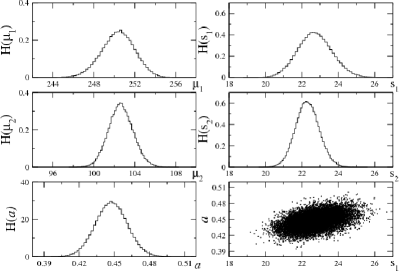
which correspond to the marginalized distributions. These marginalized distributions are depicted with histograms in Fig. 6 for the Ubiquitin.

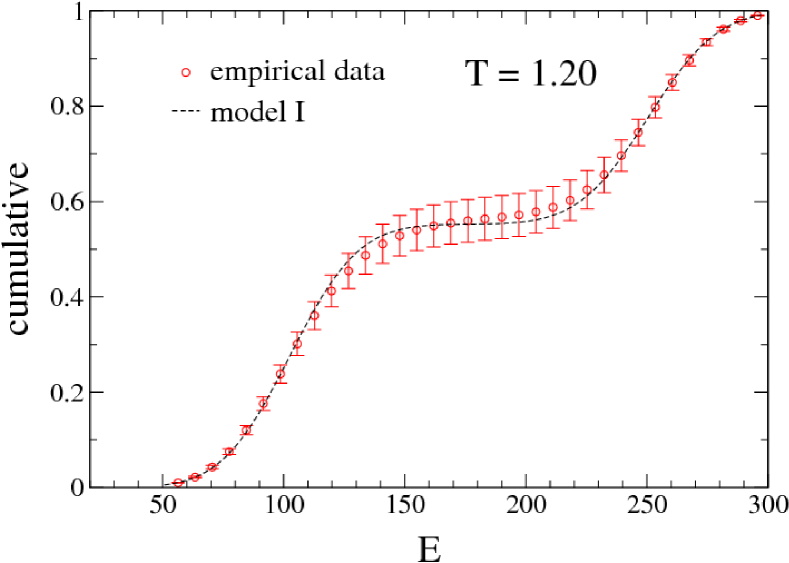
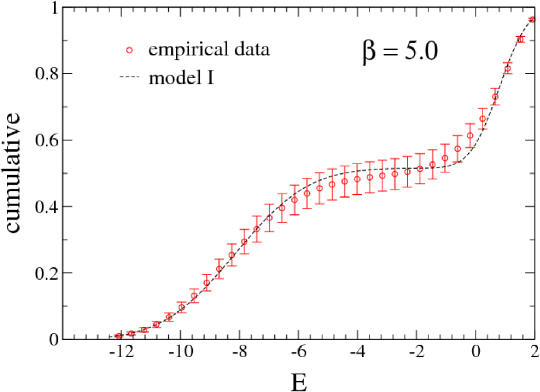
For each protein, our experimental data $\vec{y}$ is produced by dividing the observed energy range into 35 points $\{E_{i}\}$ and experimental errors are extracted from the jackknife procedure. We anticipate here that these experimental data are displayed in Figures 5 and 11 for the folding-unfolding transition of Ubiquitin and for the aggregation of two Fibonacci sequences, respectively. Within a Bayesian approach, the set of observations $\{y_{i}\}$ is just a set among possible experimental outcomes $\vec{y}$ at the points $\{E_{i}\}$. Thus, given a fixed model M and a set of experimental values $\vec{y}(\{E_{i}\})$, parameters estimation within Bayesian approach is obtained as follows bayes-caldwell ,

$$P(\vec{\lambda},\vec{\nu}\,|\,\vec{D},M)=\frac{P(\{E_{i}\}=\vec{D}\,|\,\vec{\lambda},\vec{\nu},M)\,P_{0}(\vec{\lambda},\vec{\nu}\,|\,M)}{\int P(\{E_{i}\}=\vec{D}\,|\,\vec{\lambda},\vec{\nu},M)\,P_{0}(\vec{\lambda},\vec{\nu}\,|\,M)\,d\vec{\lambda}\,d\vec{\nu}},$$ (12)

where $P_{0}(\vec{\lambda},\vec{\nu}\,|\,M)$ is the prior distribution for a fixed model M.

Since our aim is to characterise $\tilde{\beta}(E)$ in a first-order phase transition region, we assume that the energy distribution $P(E)$ (i.e. a continuous estimate for $H(E)$ in Eq. (4)) is well described by a double-peak function. This function characterises the coexistent phases at temperatures close enough to the transition temperature $T_{c}$, whose shape is a consequence of the free-energy barrier between the ordered and disordered phases. Therefore, the expected energy distribution $P(E)$ can be written as a normalized sum of two Gaussian distributions with peaks centered at energies $\mu_{1}$ and $\mu_{2}$, corresponding to the disordered and ordered phases, respectively Lee-1991 . If we assume the model M as the cumulative distribution function of $P(E)$, and recalling that for a Gaussian distribution the CDF is the error function, we arrive to the following modelling,

$$F(E)=0.5\left[1+a\,{\rm erf}\left(\frac{E-\mu_{1}}{s_{1}\sqrt{2}}\right)+(1-a)\,{\rm erf}\left(\frac{E-\mu_{2}}{s_{2}\sqrt{2}}\right)\right].$$ (13)

This is a 5-parameter model, which we call model I in our analysis, with $\vec{\lambda}=(\mu_{1},s_{1},\mu_{2},s_{2},a)$.

Now, to obtain the posterior probability of the parameter set $\vec{\lambda}$, given data set $\vec{D}$, from the likelihood $P_{i+1}(\vec{D}\,|\,\vec{\lambda})$ times the initial prior probabilities $P_{i}(\vec{\lambda})$ for our model I, we use a Markov chain Monte Carlo. To this end, we consider the Metropolis algorithm with the proposal function

$$P(\vec{D}\,|\,\vec{\lambda})=\prod_{i=1}^{35}\,\frac{1}{\sigma_{i}\sqrt{2\pi}}\,e^{-\left[y_{i}-F(E_{i})\right]^{2}/2\sigma_{i}^{2}}\,,$$ (14)

where $\sigma_{i}$ are the errors in our computational experiment. The values $F(E_{i})$ are calculated with the accepted values for the parameters $\vec{\lambda}$ of model I.

IV Numerical Comparisons

In the following, we present results where we evaluate the performance of the different approaches in obtaining continuous estimates for $H(E)$ and, consequently, the estimate $\tilde{\beta}(E)$ for microcanonical inverse temperature. The comparative analysis is made with data obtained from both MC and MD simulations, where we employ two simplified off-lattice protein models, i.e. all atoms in the polypeptide chain are replaced by beads located at the $C_{\alpha}$-atom position, and present a continuous energy spectrum.

FIG. 1: Statistical temperature estimates ${\tilde{\beta}}(E)$ of Ubiquitin using data obtained from MD simulations at $T=1.20$. Curves show the dependence of ${\tilde{\beta}}(E)$ on energy discretisations $\varepsilon$ ($\varepsilon=0.3,0.8$ and 1.3) for the linear regression method with $k=15$ points.

FIG. 2: Comparison between estimates ${\tilde{\beta}}(E)$ of Ubiquitin with the linear regression ($\varepsilon=0.8$) and CDF method for data obtained at $T=1.20$. Statistical errors for the CDF method were calculated with 20 jackknife bins.

FIG. 3: Estimates ${\tilde{\beta}}(E)$ for Ubiquitin obtained with linear regression ($\varepsilon=0.8$) and CDF method with data generated from independent MD simulations at $T=\{1.14,1.16,1.18,1.20,1.22,1.24,1.26\}$. Statistical errors for the CDF method were calculated with 80 jackknife bins.

FIG. 4: Cumulative distribution data ($\circ$) of Ubiquitin with error bars calculated with 20 jackknife bins from MD simulation at $T=1.20$. Dotted line corresponds to the Bayesian estimates of the cumulative distribution assuming model I.

FIG. 5: Energy histograms $H(E)$ for Ubiquitin. Error bars are calculated with 20 jackknife bins and are shown only for the CDF method. Inset: comparative behaviour of $dH(E)/dE$ produced with the CDF method and Bayesian approach assuming model I.

IV.1 Ubiquitin

Ubiquitin is a 76 residue small protein (PDB code 1UBQ) for which evidences suggest a two-state folding mechanism. It had received considerable attention for what concerns solvent response and temperature dependence in the secondary structure formation ubqJacob ; chung-ubiquitin ; ghosh-ubiquitin and stretching experiments jernigan-ubiquitin ; das-ubiquitin ; imparato-ubiquitin .

To study the performance of the numerical approaches in evaluating $\beta(E)$ through the folding-unfolding transition, we perform simulations with a coarse-grained version for Ubiquitin but with a rather detailed potential. We use the structure-based model implemented in SMOG@ctbp web server smog to perform MD simulations with GROMACS package. The analyses were made from $10^{6}$ measurements during 250 ns of simulation after a period of thermalization. Measurements were obtained from 7 independent simulations at temperatures $T_{\alpha}=T_{1}+(\alpha-1)\,\Delta T$ with $T_{1}=1.14$ and $\Delta T=0.02$.

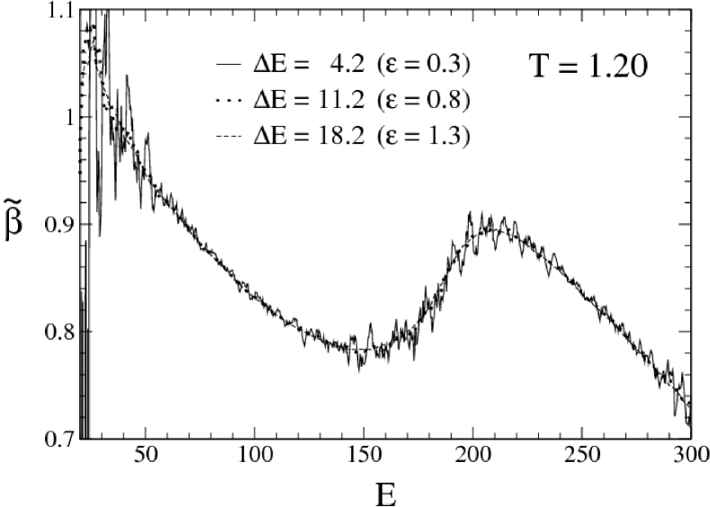
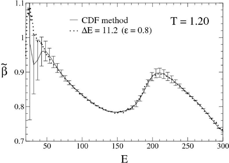
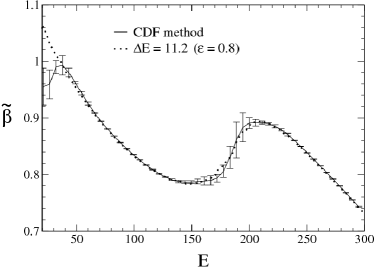
First, we evaluate the performance of the approaches considering the data obtained from a single MD trajectory produced at $T_{4}=1.20$, which is close to the transition temperature $T_{c}=1.219(3)$ evaluated with statistics obtained with 7 independent MD simulations. Figure 2 displays the estimates for the caloric curve using the linear regression to evaluate derivatives of ${\rm ln}H(E_{m})$ from data obtained at $T=1.20$. This figure shows how noisy the caloric curve can be as a function of the energy binsize $\varepsilon=0.3,0.8$ and 1.3, keeping the number of points $k=15$ fixed. Figure 2 compares what seems a good energy discretisation with the CDF method. Error bars based on 20 jackknife bins are presented only for the CDF method. Now, Fig. 3 compares both methods when we consider the statistics obtained with the entire set of temperatures $T_{\alpha}$, $(\alpha=1,2,\cdots,7)$. To present error bars for the CDF method, we have increased the number of jackknife bins to 80 because this larger statistics. Nice agreement between both methods are obtained if we choose $\varepsilon$ conveniently.

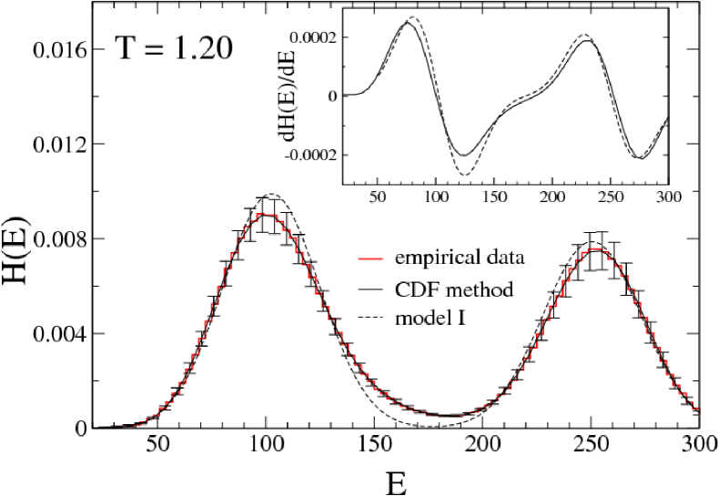
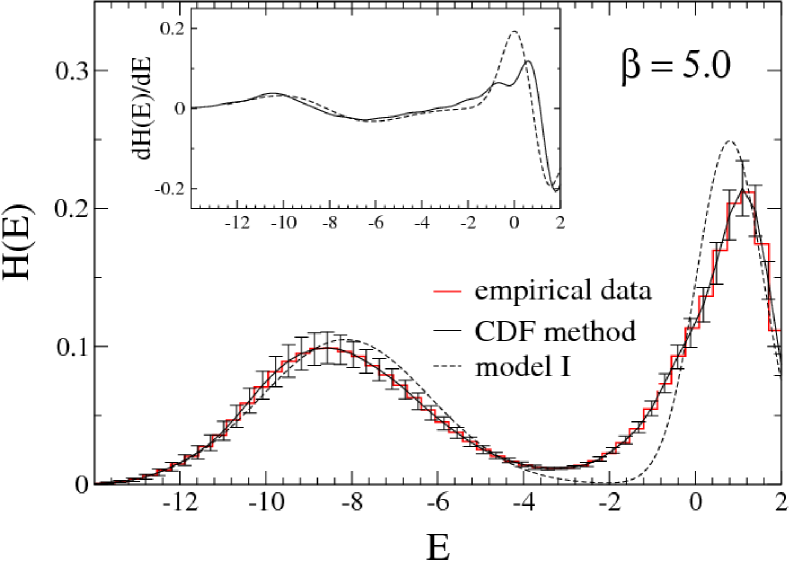
Figure 5 displays what we call input experimental points to perform the Bayesian analysis. This experimental data was obtained from MD simulations at $T=1.20$. The dashed line corresponds to the cumulative distribution obtained with model I. The parameters of this model that fit the input data are displayed in Table 1. We include values calculated from means of the marginalized distributions, and global modes that presented the smallest $\chi^{2}$/d.o.f of the model. To verify how the proposed model describes the energy distribution when compared with the CDF method and naive histogramming, we show in Fig. 5 the results obtained from these methods for the statistics collected at $T=1.20$. We realize that model I does not recover properly the region between the peaks of the energy distributions $H(E)$ obtained with previous numerical methods. The inset in this figure compares the calculations of $dH(E)/dE$ following from the CDF and Bayesian approaches. In Fig. 6 we display the marginalized distributions of $\vec{\lambda}$, including the correlation between the parameters $s_{1}$ and $a$ to illustrate their interdependence. We have always used flat priors over appropriated ranges to obtain the parameter distributions.

FIG. 6: Marginalized PDFs of the parameters for model I, and scatter plot for joint probability of $a$ and $s_{1}$ with data obtained for Ubiquitin at $T=1.20$.

IV.2 Fibonacci sequences

Figure 8 shows the caloric curve for the aggregation of two chains of monomers described by the AB model, a coarse-grained off-lattice protein model that replaces the all-atom potentials by simpler physical interactions. This model reduces the protein to a chain of monomers of two types: the hydrophobic ($A$) and the polar or hydrophilic ($B$) types, located at the $C_{\alpha}$ atoms. The AB model has also been used in studies to explore aggregation phenomenon jankePRL2006 ; jankeJCP2008 , where more than one chain is included in the system, and in studies of microcanonical thermostatistics of heteropolymers frigoriJCP2013 .

Here, we consider a simple system which consists of two heteropolymers defined by Fibonacci sequences with $13$ monomers, i.e. ABBABBABABBAB. The statistics for this system amounts to $10^{7}$ sweeps per replica produced with REM. Attempts to exchange the replicas occur every $n_{s}=10^{4}$ sweeps, using a scheme that alternates attempts between even replicas and their neighbors, and odd replicas and their neighbors. Although one has several manners to define the temperature set fiore , here we determine it using an arithmetic progression $\beta_{\alpha}=\beta_{1}+(\alpha-1)\,\Delta\beta$. We consider $N_{\rm rep}=7$ replicas choosing $\beta_{1}=4.2$, and $\Delta\beta=0.4$.

FIG. 7: Estimates ${\tilde{\beta}}(E)$ for the aggregation of two Fibonacci sequences for different parameters $\varepsilon$ and $k=15$ points with data selected for $\beta=5.0$ among time series produced with REM.

FIG. 8: Comparison between estimates ${\tilde{\beta}}(E)$ for the aggregation of two Fibonacci sequences with the linear regression ($\varepsilon=0.05$) and CDF method for data obtained at $\beta=5.0$. Statistical errors for the CDF method were calculated with 20 jackknife bins.

FIG. 9: Comparison between estimates ${\tilde{\beta}}(E)$ for the aggregation of two Fibonacci sequences with the linear regression ($\varepsilon=0.05$) and CDF method for energy time series obtained from REM at $\beta=\{4.2,4.6,5.0,5.4,5.8,6.2,6.6\}$.

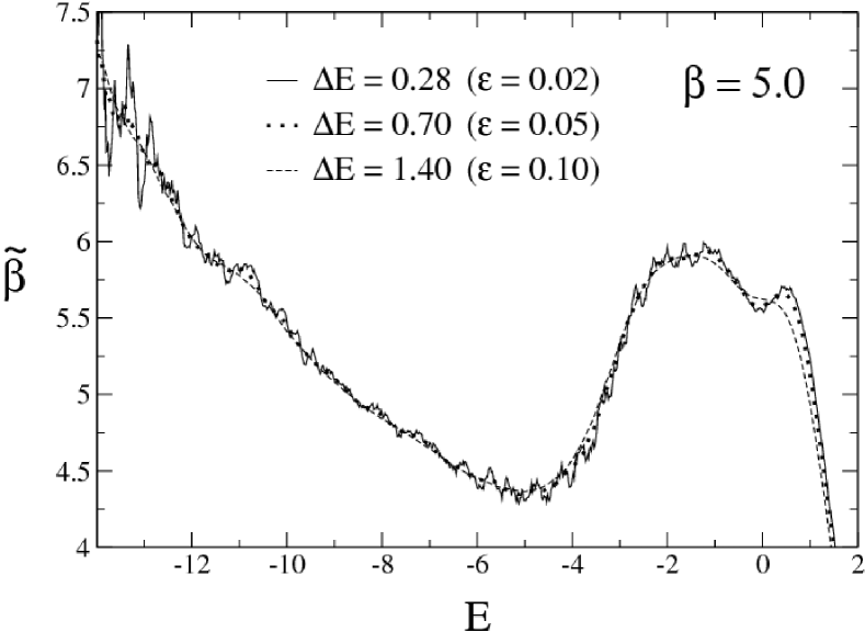
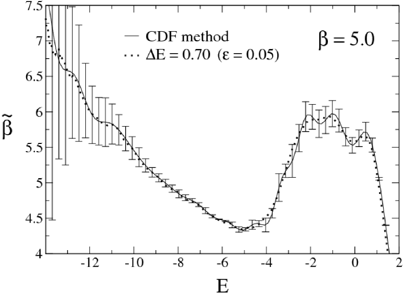
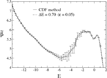
Figure 8 depicts the caloric curves ${\tilde{\beta}}(E)$ obtained with energy binsizes $\varepsilon=0.02,0.05$, and $0.10$. The value $k=15$ was used to calculate the derivatives of ${\rm ln}H(E_{m})$. Different values of $\varepsilon$ allows one to verify the systematic errors associated with $\varepsilon$ and the use of linear regression. For a fixed $k$, small values of $\varepsilon$ (or $\Delta E$) tend to reproduce the statistical fluctuations of the data. On the other hand, a value as large as $\varepsilon=0.10$ eliminates the physical information associated with the small S-loop at $E\sim 0.2$. For comparison, we include in Fig. 8 the ${\tilde{\beta}}(E)$ estimates from the CDF method. These comparisons are based on a single time series selected from data produced with REM at the inverse temperature $\beta=5.0$. It is important to reliably calculate the caloric curve when assessing the canonical critical temperature and the latent heat of the transition. We can figure out how important the fluctuations observed in these curves ${\tilde{\beta}}(E)$ are by calculating the statistical errors associated with the CDF method. Figure 8 displays the statistical error bars calculated with 20 jackknife bins for the dataset with $10^{7}$ measurements obtained with REM at $\beta=5.0$. Both methods present comparable statistical error bars. This figure shows that the small S-loop at $E\sim 0.2$ does not result from the statistical fluctuations in our dataset. Therefore, any smooth estimate of this curve at $E\sim 0.2$, obtained for example with $\Delta E=1.40$ ($\varepsilon=0.10$), would hide physical information.

FIG. 10: Cumulative distribution data ($\circ$) for the aggregation of two Fibonacci sequences with error bars calculated with 20 jackknife bins from REM simulation for the energy time series obtained at $\beta=5.0$. Dotted line corresponds to the Bayesian estimates of the cumulative distribution assuming model I.

FIG. 11: Comparison of energy histograms $H(E)$ for the aggregation of two Fibonacci sequences. Error bars are calculated with 20 jackknife bins are shown for the CDF method. Inset: comparative behaviour of $dH(E)/dE$ as predicted with the CDF method and Bayesian analysis assuming model I.

In Fig. 9 we include data produced with $N_{\rm rep}=7$ replicas together. Comparison of the results presented in this figure with those obtained by multicanonical simulations in Refs. jankePRL2006 ; jankeJCP2008 reveals that they are in excellent agreement: even the small S-loop near $E\sim 0.2$ appears in our case. Computation of the inverse of aggregation temperature $\beta_{\rm agg}=5.212(59)$ also resulted in a quantitative agreement. Larger error bars appear around $E=-4$, probably because the lack of temperatures in the set used to exchange the replicas. The averaged estimates from both derivative calculation methods agreed for a particular choice of $\varepsilon=0.05$ and $k=15$ points in the linear regression method.

Now, Fig. 11 shows the experimental data we have used to perform the Bayesian analysis. Again, we initially keep the analysis restricted to a single energy time series, in this case produced at $\beta=5.0$. We have included the Bayesian estimates (dashed line) of the cumulative function assuming the model I. The parameters for this model are presented in Table I. To verify how well this model reproduces $P(E)$, we include in Fig. 11 the energy distributions obtained with a naive histogramming procedure, CDF method and Bayesian analysis. Clearly, Bayesian analysis does not reproduce the expected behaviour between both peaks. This leads to a biased estimation of $dH(E)/dE$ as can be seem in the inset of this figure. Moreover, the approach with model I does not reproduce the small S-loop observed at $E\sim 0.2$ (data not shown), in contrast to the estimates with a convenient choice of $\varepsilon$ or the CDF method. As a consequence, we again do not follow further analysis with the Bayesian approach including all statistics from the 7 replicas.

V Summary and conclusions

We presented two alternative approaches for the estimation of the energy probability distributions avoiding the need of energy binning in order to obtain the microcanonical thermostatistics analysis from ST-WHAM. Numerical comparisons between the approaches were presented and we showed the statistical and systematic errors that can arise when one evaluates the microcanonical inverse temperature for two continuous energy models that exhibits first-order like phase transitions. Our results indicate that the CDF method yields reliable estimates for both $H(E)$ and $\beta(E)$ when compared with the linear regression method, and far more successfully than the Bayesian approach with model I. Unlike the linear regression method, the CDF method avoids the undesirable task of choosing the energy binsize $\varepsilon$ for a careful evaluation of the microcanonical temperature, as highlighted in the analysis of the aggregation transition of the two Fibonacci sequences. In this case, the caloric curve presents a quite unusual behaviour with two S-loops, indicating two transitions. In particular, we showed that the use of large values for $\varepsilon$ in linear regression method would hide physical information about the small S-loop at $E\sim 0.2$. On the other hand, the small S-loop could not be detected with the Bayesian analysis (data not shown) as a consequence of the poor evaluation of $H(E)$ and its derivative (Fig. 11). The reason is because the model I consists of only 5 parameters. This is a low number compared to the CDF method, which allows a variable number of parameters (i.e. Fourier coefficients) defined depending on the demand of the ECDF. For instance, the CDF method needs 13 Fourier coefficients to obtain probability densities for the Ubiquitin data and this number goes up to 74 for Fibonacci sequences. Furthermore, model I was constructed on the hypothesis that the coexistence of two thermodynamic bulk phases can be well described by two gaussian distributions. Actually, this is an approximation because the energies in between the two peaks, describing mixed phase configurations, are not properly take into account in the two gaussian model.

VI Appendix

Derivative of the probability density:

 FUNCTION DERPD(X)
 include ’../../Libs/Fortran/implicit.sta’
 include ’../../Libs/Fortran/constants.par’
 PARAMETER(NMAX=100)
 COMMON /CDFProb/ XMIN,XRANGE,DN(NMAX),M
!M    number of Fourier coefficients
 DERPD=ZERO
 DO J=1,M
   AUX=J*PI/XRANGE
   AUX=AUX*AUX
   DERPD=DERPD-DN(J)*AUX*SIN(J*PI/XRANGE*(X-XMIN))
 ENDDO
 RETURN
 END

Examples		$\mu_{1}$	$s_{1}$	$\mu_{2}$	$s_{2}$	$a$	$\chi^{2}$/d.o.f.
Ubiquitin	mean	250.36(37)	22.73(22)	102.64(27)	22.31(15)	0.4474(31)	0.131
	global mode	250.51	22.64	102.55	22.27	0.4474	0.130
Fibonacci	mean	0.797(15)	0.7786(79)	-8.128(37)	1.968(25)	0.4838(35)	0.350
sequences	global mode	0.803	0.7754	-8.147	1.958	0.4841	0.349

Table 1: Parameters for the proposed model in Eq. (13) from averages and the $\chi^{2}$/d.o.f of the model.

References

- (1) D.H.E. Gross, Microcanonical thermodynamics: phase transitions in small systems, Lecture Notes in Physics 66 (World Scientific, Singapore, 2001).
- (2) D.H. Gross, and J.F. Kenney, J. Chem. Phys. 122 (2005) 224111.
- (3) R.B. Frigori, L.G. Rizzi, and N.A. Alves, J. Phys.: Conf. Ser. 246 (2010) 012018.
- (4) S. Schnabel, D.T. Seaton, D.P. Landau, and M. Bachmann, Phys. Rev. E 84 (2011) 011127.
- (5) J.C.S. Rocha, S. Schnabel, D.P. Landau, and M. Bachmann, Phys. Rev. E 90 (2014) 022601.
- (6) R.B. Frigori, L.G. Rizzi, and N.A. Alves, J. Chem. Phys. 138 (2013) 015102.
- (7) C. Junghans, M. Bachmann, and W. Janke, Phys. Rev. Lett. 97 (2006) 218103.
- (8) C. Junghans, M. Bachmann, H. Arkin, and W. Janke, J. Chem Phys. 128 (2008) 085103.
- (9) M. Möddel, W. Janke, and M. Bachmann, Phys. Chem. Chem. Phys. 12 (2010) 11548.
- (10) T. Bereau, M. Bachmann, and M. Deserno, J. Am. Chem. Soc. 132 (2010) 13129.
- (11) M.S. Church, C.E. Ferry and A. E. van Giessen, J. Chem. Phys. 136 (2012) 245102.
- (12) W.J. Cho, J. Kim, J. Lee, T. Keyes, J.E. Straub, and K.S. Kim, Phys. Rev. Lett. 112 (2014) 157802.
- (13) A. Mitsutake, Y. Sugita, and Y. Okamoto, Biopolymers 60 (2001) 96.
- (14) D.P. Landau, and K. Binder, A guide to Monte Carlo simulations in Statistics Physics. Cambridge University Press, 2000.
- (15) B.A. Berg, 2000. Monte Carlo Methods, Fields Institute Communications Vol. 26, edited by N. Madras (American Mathematical Society, Providence, RI, 2000), p. 1-24.
- (16) B.A. Berg, Comput. Phys. Commun. 153 (2003) 397.
- (17) R.S. Johal, and A. Planes, E. Vives, Phys. Rev. E 68 (2003) 056113.
- (18) T. Neuhaus, and J.S. Hager, Phys. Rev. E 74 (2006) 036702.
- (19) R.B. Frigori, L.G. Rizzi, and N.A. Alves, Eur. Phys. J. B 75 (2010) 311.
- (20) I. Andricioaei, and J.E. Straub, Phys. Rev. E 53 (1996) R3055.
- (21) U.H.E. Hansmann, and Y. Okamoto, Phys. Rev. E 56 (1997) 2228.
- (22) K. Hukushima, and K. Nemoto, J. Phys. Soc. Japan 65 (1996) 1604.
- (23) J. Kim, T. Keyes, and J.E. Straub, J. Chem. Phys. 132 (2010) 224107.
- (24) A.M. Ferrenberg, and R.H. Swendsen, Phys. Rev. Lett. 61 (1988) 2635. [Erratum: 63 (1989) 1658]
- (25) A.M. Ferrenberg, and R.H. Swendsen, Phys. Rev. Lett. 63 (1989) 1195.
- (26) N.A. Alves, B.A. Berg, and S. Sanielevici, Nucl. Phys. B 376 (1992) 218.
- (27) J. Kim, T. Keyes, and J.E. Straub, J. Chem. Phys. 135 (2011) 061103.
- (28) L.G. Rizzi, and N.A. Alves, J. Chem. Phys. 135 (2011) 141101.
- (29) B.A. Berg, and R.C. Harris, Comput. Phys. Commun. 179 (2008) 443.
- (30) A. Caldwell, D. Kollár, and K. Kröninger, Comput. Phys. Comm. 180 (2009) 2197.
- (31) W. Press et al., Numerical Recipes (Cambridge University Press, London, 1986).
- (32) J. Lee, and J.M. Kosterlitz, Phys. Rev. B 43 (1991) 3265.
- (33) J. Jacob, B. Krantz, R.S. Dothager, P. Thiyagarajan, and T.R. Sosnick, J. Mol. Biol. 338 (2004) 369.
- (34) H.S. Chung, and A. Tokmakoff, Proteins 72 (2008) 474.
- (35) S.G. Dastidar, and C. Mukhopadhyay, Phys. Rev. E 72 (2005) 051928.
- (36) J.I. Sulkowska, A. Kloczkowski, T.Z. Sen, M. Cieplak, R.L. Jernigan, Proteins 71 (2008) 45.
- (37) A. Das, C. Mukhopadhyay, Proteins 75 (2009) 1024.
- (38) A. Imparato, A. Pelizzola, Phys. Rev. Lett. 100 (2008) 158104.
- (39) J.K. Noel, P.C. Whitford, K.Y. Sanbonmatsu, and J.N. Onuchic, Nucl. Acids Res. 38 (2010) W657.
- (40) C.E. Fiore, J. Chem. Phys. 135 (2011) 114107.