Weighted polynomial approximation
of rational Bézier curves^∗

Abstract. We present an efficient method to solve the problem of the constrained least squares approximation of the rational Bézier curve by the Bézier curve. The presented algorithm uses the dual constrained Bernstein basis polynomials, associated with the Jacobi scalar product, and exploits their recursive properties. Examples are given, showing the effectiveness of the algorithm.

AMS classification: Primary 41A10. Secondary 65D17, 33D45

Keywords: Rational Bézier curve; Polynomial approximation; Constrained dual Bernstein basis.

1. Introduction

In CAGD, it is frequently important to approximate a rational Bézier curve by a polynomial one. In the last two decades, many approaches to this problem have been proposed [18, 19, 15, 5, 10, 17, 7]. The large spectrum of methods contains approximation by hybrid curves [18, 19, 15], Hermite interpolation [5, 15], progressive iteration approximation [17], least squares approximation [10] and approximation by Bézier curves with the control points obtained by successive degree elevation of the rational Bézier curve [7].

In this paper, we consider the following approximation problem.

Problem 1.1.

Let be given a rational Bézier curve $R_{n}$ of degree $n$, with control points $r_{i}\in\mathbb{R}^{d}$ and positive weights $\omega_{i}\in\mathbb{R}$,

(1.1) $$R_{n}(t)=\dfrac{Q_{n}(t)}{\omega(t)}=\frac{\sum_{i=0}^{n}\omega_{i}r_{i}\,B^{n}_{i}(t)}{\sum_{i=0}^{n}\omega_{i}\,B^{n}_{i}(t)}\qquad(0\leq t\leq 1),$$

where

$$B^{n}_{i}(t)=\binom{n}{i}t^{i}(1-t)^{n-i}\qquad(0\leq i\leq n)$$

are Bernstein basis polynomials. Find a degree $m$ Bézier curve

(1.2) $$P_{m}(t)=\sum_{i=0}^{m}p_{i}\,B^{m}_{i}(t)\qquad(0\leq t\leq 1)$$

such that the value of the error

(1.3) $$\int_{0}^{1}(1-t)^{\alpha}t^{\beta}\,\|R_{n}(t)-P_{m}(t)\|^{2}\mbox{$\mbox{${\rm\,d}$}t$}\qquad(\alpha,\;\beta>-1)$$

is minimized in the space $\Pi^{d}_{m}$ of parametric polynomials in $\mathbb{R}^{d}$ of degree at most $m$ (for simplicity, we write $\Pi_{m}:=\Pi^{1}_{m}$) under the additional conditions that

(1.4) $$\left\{\begin{array}[]{l}R_{n}^{(i)}(0)=P_{m}^{(i)}(0)\qquad(i=0,1,\ldots,k-1),\\[8.61108pt] R_{n}^{(j)}(1)=P_{m}^{(j)}(1)\qquad(j=0,1,\ldots,l-1),\end{array}\right.$$

where $k+l\leq m$. Here $\|\cdot\|$ is the Euclidean vector norm.

Note that in the case $\alpha=\beta=0$, the above problem as well the method proposed in this paper reduce to the form given in [14].

The values of $n$ and $m$ are not related. However, if $(m+1)d<(n+1)(d+1)$ then the number of parameters of the approximating polynomial curve is smaller than the total number of parameters of the rational curve.

In [10], an approximate solution to the above problem with $m>n$ is obtained by solving a linear least squares problem. Paper [2] deals with more general problem of the constrained degree reduction of rational Bézier curves; one of the auxiliary problems discussed there contains the above problem as a particular case. We present a method which is based on the idea of using constrained dual Bernstein polynomial basis [20] to compute the control points $p_{i}$. Our algorithm is efficient thanks to using fast schemes of $1^{o}$ evaluation the Bézier form coefficients of the dual polynomials [13] and $2^{o}$ numerical computation of the collection of integrals

$$\int_{0}^{1}\frac{(1-t)^{\alpha}t^{\beta}B^{n+m}_{h}(t)}{\omega(t)}\mbox{$\mbox{${\rm\,d}$}t$}\qquad(k\leq h\leq n+m-l).$$

The cost is significantly lower than in the case of the special variant of the method of [2], which needs inverting a $(n+m-k-l+1)\times(n+m-k-l+1)$ matrix.

Let us mention that the problem stated above can be also considered for other norms. However, even the simpler problem of constrained degree reduction of Bézier curves in $L_{\infty}$-norm requires higher computational complexity (see, e.g., [1]). The most appropriate metric for curves in geometric terms would be the Hausdorff distance, but the computation of such distance of the nonlinear curves is not so easy. Hence, $L_{2}$-norm seems to be a good choice as we can construct solution in explicit form using the Bernstein and dual Bernstein bases in a natural and convenient way.

The outline of this paper is as follows. Section 2 contains basic facts on the constrained dual Bernstein polynomials. Section 3 brings a complete solution to Problem 1.1; for implementation details, see Section 4. In Section 5, the proposed method is applied to some examples and compared with two other algorithms.

2. Constrained dual Bernstein polynomials

Let $\Pi_{m}^{(k,l)},$where $k+l\leq m$, be the space of all polynomials of degree $\leq m$, whose derivatives of order $\leq k-1$ at $t=0$, as well as derivatives of order $\leq l-1$ at $t=1$, vanish:

$$\Pi_{m}^{(k,l)}:=\left\{P\in\Pi_{m}\>:\>P^{(i)}(0)=0\quad(0\leq i\leq k-1)\;\mbox{and}\;P^{(j)}(1)=0\quad(0\leq j\leq l-1)\right\}.$$

Obviously, $\mbox{dim}\;\Pi_{m}^{(k,l)}=m-k-l+1$, and the Bernstein polynomials $\left\{B^{m}_{k},B^{m}_{k+1},\ldots,B^{m}_{m-l}\right\}$ form a basis of this space. There is a unique dual constrained Bernstein basis of degree $m$,

$$D^{(m,k,l)}_{k}(x;\alpha,\beta),\,D^{(m,k,l)}_{k+1}(x;\alpha,\beta),\ldots,D^{(m,k,l)}_{m-l}(x;\alpha,\beta),$$

satisfying

$$\langle D^{(m,k,l)}_{i},\,B^{m}_{j}\rangle=\delta_{ij}\qquad(i,j=k,k+1,\ldots,m-l),$$

where $\delta_{ij}$ is 1 if $i=j$ and 0 otherwise, and the inner product $\langle\cdot,\cdot\rangle$ is given by

$$\langle f,\,g\rangle:=\int_{0}^{1}(1-t)^{\alpha}t^{\beta}f(t)g(t)\mbox{$\mbox{${\rm\,d}$}t$}\qquad(\alpha,\,\beta>-1).$$

Properties of the polynomials $D^{(m,k,l)}_{i}$ are studied in [12, 13] and [20]. We need the following result.

Theorem 2.1 ([13]).

The constrained dual basis polynomials have the Bézier-Bernstein representation

(2.1) $$D^{(m,k,l)}_{i}(x;\alpha,\beta)=\sum_{j=k}^{m-l}c_{ij}(m,k,l,\alpha,\beta)\,B^{m}_{j}(x),$$

where the coefficients $c_{ij}\equiv c_{ij}(m,k,l,\alpha,\beta)$ satisfy the recurrence relation

(2.2) $$c_{i+1,j}= \frac{1}{A(i)}\,\left\{(i-j)(2i+2j-2m-\alpha+\beta)\,c_{ij}\right.$$

$$\hphantom{\frac{1}{A(i)}\,\{}\left.+B(j)\,c_{i,j-1}+A(j)\,c_{i,j+1}-B(i)\,c_{i-1,j}\right\}$$

$$\hphantom{\frac{1}{A(i)}\,\{+B(j)\,c_{i,j-1}+A(j)\,c_{i,j+1}}(k\leq i\leq m-l-1,\quad k\leq j\leq m-l)$$

with

$$\begin{array}[]{l}A(u):=(u-m)(u-k+1)(u+k+\beta+1)/(u+1),\\[8.61108pt] B(u):=u(u-m-l-\alpha-1)(u-m+l-1)/(u-m-1).\end{array}$$

We adopt the convention that $c_{ij}:=0$ if $i<k$, or $i>m-l$, or $j<k$, or $j>m-l$. The starting values are

(2.3) $$c_{kj}= \mbox{$\displaystyle\binom{m}{k}^{\!\!-1}\!\!$}\,\frac{(-1)^{k}(\sigma+2k+2l+1)_{m-k-l}(k+\beta+2)_{m-l}}{(m-k-l)!B(\alpha+2l+1,\,\beta+2k+1)}$$

$$\times\binom{m-k-l}{j-k}\mbox{$\displaystyle\binom{m}{j}^{\!\!-1}\!\!$}\,\,\frac{(-1)^{j}}{(\alpha+2l+1)_{m-l-j}(k+\beta+2)_{j}},$$

where $j=k,k+1,\ldots,m-l$, and we use the notation

$$(a)_{k}:=\prod_{j=0}^{k-1}(a+j)\quad(k\geq 0),\qquad\sigma:=\alpha+\beta+1,\qquad B(\lambda,\,\mu)=\frac{\Gamma(\lambda)\Gamma(\mu)}{\Gamma(\lambda+\mu)}.$$

Observe that the quantities $c_{ij}$ can be put in a square table (see Table 1).

Table 1. The $c$-table

$$\begin{array}[]{cccccc}&0&0&\ldots&0&\\[8.61108pt] 0&c_{kk}&c_{k,k+1}&\ldots&c_{k,m-l}&0\\[8.61108pt] 0&c_{k+1,k}&c_{k+1,k+1}&\ldots&c_{k+1,m-l}&0\\[8.61108pt] \lx@intercol\dotfill\hfil\hfil\lx@intercol\\[8.61108pt] 0&c_{m-l,k}&c_{m-l,k+1}&\ldots&c_{m-l,m-l}&0\\[8.61108pt] &0&0&\ldots&0&\end{array}$$

Now, the $c$-table can be completed very easily in the following way.

Algorithm 2.2 (Computing the coefficients $c_{ij}(m,k,l,\alpha,\beta)$ [13]).

I:

Compute recursively quantities $c_{kk},\;c_{k,k+1},\ldots,\,c_{k,m-l},$ filling the first row of the $c$-table, by the formulas

(2.4) $$c_{k,m-l}:= \mbox{$\displaystyle\binom{m}{k}^{\!\!-1}\!\!$}\,\mbox{$\displaystyle\binom{m}{l}^{\!\!-1}\!\!$}\;\frac{(-1)^{m-k-l}(\sigma+2k+2l+1)_{m-k-l}}{B(\alpha+2l+1,\,\beta+2k+1)\,(m-k-l)!},$$

(2.5) $$c_{kj}:= \frac{(j-m)(j-k+1)(j+\beta+k+2)}{(j+1)(j-m+l)(j-\alpha-l-m)}\,c_{k,j+1}$$

$$\hphantom{\frac{(j-n)(j-k+1)(j+\beta+k+2)}{(j+1)(j-n+l)(j-\alpha-l-n)}}(j=m-l-1,m-l-2,\ldots,k).$$

II:

For $i=k,k+1,\ldots,m-l-1$ and $j=k,k+1,\ldots,m-l$, compute $c_{i+1,j}$, using the recurrence (2.2).

3. Constrained polynomial approximation of rational Bézier curve

Clearly, the Bézier curve being the solution of Problem 1.1 can be obtained in a componentwise way. Hence, it is sufficient to give the details of our method of solving this problem in case where $R_{n},\;P_{m}\in\mathbb{R}^{1}$.

Given the rational function

(3.1) $$R_{n}(t)=\dfrac{Q_{n}(t)}{\omega(t)}=\frac{\sum_{i=0}^{n}\omega_{i}r_{i}\,B^{n}_{i}(t)}{\sum_{i=0}^{n}\omega_{i}\,B^{n}_{i}(t)}\qquad(0\leq t\leq 1),$$

with $r_{i}\in\mathbb{R}$ and $\omega_{i}\in\mathbb{R}_{+}$, we look for a degree $m$ polynomial

(3.2) $$P_{m}(t)=\sum_{i=0}^{m}p_{i}\,B^{m}_{i}(t)\qquad(0\leq t\leq 1)$$

which gives the minimum value of

(3.3) $$\|R_{n}(t)-P_{m}(t)\|^{2}_{L_{2}}=\langle R_{n}-P_{m},R_{n}-P_{m}\rangle$$

with the constraints

(3.4) $$\begin{array}[]{l}R_{n}^{(i)}(0)=P_{m}^{(i)}(0)\qquad(i=0,1,\ldots,k-1),\\[8.61108pt] R_{n}^{(j)}(1)=P_{m}^{(j)}(1)\qquad(j=0,1,\ldots,l-1),\end{array}$$

where $k+l\leq m$.

Theorem 3.1.

Given the coefficients $r_{0},r_{1},\ldots,r_{n}$ and weights $\omega_{0},\omega_{1},\ldots,\omega_{n}$ of the rational function (3.1), the coefficients $p_{0},p_{1},\ldots,p_{m}$ of the polynomial (3.2) minimising the error (3.3) with constraints (3.4) are given by

(3.5) $$p_{i}= \frac{(m-i)!}{m!}\varrho_{i0}-\sum_{j=0}^{i-1}(-1)^{i+j}\binom{i}{j}p_{j}\qquad(i=0,1,\ldots,k-1);$$

(3.6) $$p_{m-i}= (-1)^{i}\frac{(m-i)!}{m!}\varrho_{i1}-\sum_{j=1}^{i}(-1)^{j}\binom{i}{j}p_{m-i+j}\qquad(i=0,1,\ldots,l-1);$$

(3.7) $$p_{i}= \sum_{h=0}^{n}\binom{n}{h}\omega_{h}\,r_{h}\,\sum_{j=k}^{m-l}\binom{m}{j}\mbox{$\displaystyle\binom{n+m}{j+h}^{\!\!-1}\!\!$}\,c_{ij}(m,k,l,\alpha,\beta)I_{j+h}$$

$$-\left(\sum_{j=0}^{k-1}+\sum_{j=m-l+1}^{m}\right)p_{j}\,K_{ij}\qquad(i=k,k+1,\ldots,m-l),$$

where $c_{ij}(m,k,l,\alpha,\beta)$ are introduced in (2.1), while $\varrho_{i0}$ and $\varrho_{i1}$ are defined recursively for $i=0,1,\ldots$ by

(3.8) $$\varrho_{i0}:= \frac{n!}{\omega_{0}}\left[\frac{1}{(n-i)!}\Delta^{i}\left(\omega_{0}r_{0}\right)-\sum_{j=0}^{i-1}\binom{i}{j}\frac{\Delta^{i-j}\omega_{0}}{(n-i+j)!}\,\varrho_{j0}\right];$$

(3.9) $$\varrho_{i1}:= \frac{n!}{\omega_{n}}\left[\frac{1}{(n-i)!}\Delta^{i}\left(\omega_{n-i}r_{n-i}\right)-\sum_{j=0}^{i-1}\binom{i}{j}\frac{\Delta^{i-j}\omega_{n-i+j}}{(n-i+j)!}\,\varrho_{j1}\right],$$

and

(3.10) $$I_{h}:= \int_{0}^{1}\frac{(1-t)^{\alpha}t^{\beta}B^{n+m}_{h}(t)}{\omega(t)}\,\mbox{$\mbox{${\rm\,d}$}t$},$$

(3.11) $$K_{ij}= \binom{m}{j}\mbox{$\displaystyle\binom{m}{i}^{\!\!-1}\!\!$}\,\frac{(-1)^{i-k}(k-j)_{m-k-l+1}}{(i-j)(i-k)!(m-l-i)!}$$

$$\times\frac{(\alpha+l+1)_{m-j}(\beta+k+1)_{j}}{(\alpha+l+1)_{m-i}(\beta+k+1)_{i}}.$$

Here we use the standard notation $\Delta^{0}c_{h}=c_{h}$, $\Delta^{j}c_{h}=\Delta^{j-1}c_{h+1}-\Delta^{j-1}c_{h}$ ($j=1,2,\ldots$).

Proof. Recall that for arbitrary polynomial of degree $N$,

$$U_{N}(t)=\sum_{i=0}^{N}u_{i}\,B^{N}_{i}(t),$$

the well-known formulas hold (see, e.g., [4, p. 49])

$$U^{(j)}_{N}(0) = \frac{N!}{(N-j)!}\Delta^{j}u_{0}=\frac{N!}{(N-j)!}\sum_{h=0}^{j}(-1)^{j+h}\binom{j}{h}u_{h},$$

$$U^{(j)}_{N}(1) = \frac{N!}{(N-j)!}\Delta^{j}u_{N-j}=\frac{N!}{(N-j)!}\sum_{h=0}^{j}(-1)^{j+h}\binom{j}{h}u_{N-j+h}.$$

Using them in

$$R^{(i)}_{n}(h)=\frac{1}{\omega(h)}\left[Q^{(i)}_{n}(h)-\sum_{j=0}^{i-1}\binom{i}{j}R^{(j)}_{n}(h)\omega^{(i-j)}(h)\right]\quad(h=0,1)$$

gives equations (3.8), (3.9), where we denoted

$$\varrho_{ih}:=R^{(i)}_{n}(h).$$

Using the above equations in (3.4), we obtain the forms (3.5) and (3.6) for the coefficients $p_{0},\,p_{1},\ldots,p_{k-1}$ and $p_{m-l+1},\ldots,p_{m-1},p_{m}$, respectively.

The remaining coefficients $p_{i}$ are to be determined so that

$$\|R_{n}-P_{m}\|^{2}_{L_{2}}=\|W-\sum_{i=k}^{m-l}p_{i}B^{m}_{i}\|^{2}_{L_{2}}$$

has the least value, where

$$W:=R_{n}-\left(\sum_{j=0}^{k-1}+\sum_{j=m-l+1}^{m}\right)p_{j}B^{m}_{j}.$$

Remembering that $B^{m}_{i}$ and $D^{(m,k,l)}_{i}$ ($k\leq i\leq m-l$) are dual bases in the space $\Pi_{m}^{(k,l)}$, we obtain the formula

$$p_{i}= \left\langle{W},{D^{(m,k,l)}_{i}}\right\rangle$$

$$= \sum_{j=k}^{m-l}c_{ij}(m,k,l,\alpha,\beta)\,\langle R_{n},\,B^{m}_{j}\rangle-\left(\sum_{j=0}^{k-1}+\sum_{j=m-l+1}^{m}\right)p_{j}\mbox{$\left\langle{B^{m}_{j}},{D^{(m,k,l)}_{i}}\right\rangle$}.$$

Observe that

$$\langle R_{n},\,B^{m}_{j}\rangle= \sum_{h=0}^{n}\omega_{h}\,r_{h}\langle{B^{n}_{h}}/{\omega},\,B^{m}_{j}\rangle$$

$$= \sum_{h=0}^{n}\omega_{h}\,r_{h}\binom{n}{h}\binom{m}{j}\mbox{$\displaystyle\binom{m+n}{h+j}^{\!\!-1}\!\!$}\langle 1/{\omega},\,B^{m+n}_{h+j}\rangle$$

$$= \sum_{h=0}^{n}\omega_{h}\,r_{h}\binom{n}{h}\binom{m}{j}\mbox{$\displaystyle\binom{m+n}{h+j}^{\!\!-1}\!\!$}I_{h+j},$$

where we use notation (3.10).

Using results of [20] and [12], we deduce that

$$K_{ij}:= \left\langle{B^{m}_{j}},{D^{(m,k,l)}_{i}}\right\rangle$$

$$= \binom{m}{j}\mbox{$\displaystyle\binom{m}{i}^{\!\!-1}\!\!$}\,\frac{(\alpha+l+1)_{m-j}(\beta+k+1)_{j}}{(i-k)!(m-l-i)!(\alpha+l+1)_{l}(\beta+k+1)_{k}}$$

$$\times d_{i-k}(j-k;\beta+2k,\alpha+2l,m-k-l),$$

where for $h=0,1,\ldots,N$ we define

$$d_{h}(x;a,b,N)=\lim_{n\to N}\,\frac{(-1)^{h}\,N!}{n!(a+1)_{h}(b+1)_{n-h}}\,\sum_{v=0}^{h}\frac{(-h)_{v}\,(v+1-N)_{n-v}(b+1)_{n-v}}{(n+a+b+2)_{N-v}}$$

$$\hphantom{d_{h}(x;a,b,N)=\lim_{n\to N}\,\times\sum_{v=0}^{h}\frac{(-h)_{v}\,(b+1)_{n-v+2}}{a}}\times\,Q_{n-v}(N-x;b,a+v+1,N-v-1)$$

with

$$Q_{p}(t;\mu,\nu,M):=\sum_{u=0}^{p}\frac{(-p)_{u}(p+\mu+\nu+1)_{u}(-t)_{u}}{u!(\mu+1)_{u}(-M)_{u}}$$

being Hahn polynomials (see, e.g., [9, §9.5]). It is easy to see that

$$d_{h}(x;a,b,N)=\frac{(-x)_{N+1}(-N-b)_{h}}{(h-x)(a+1)_{h}(b+1)_{N}}\qquad(0\leq h\leq N).$$

Hence, some algebra gives

$$K_{ij}= \binom{m}{j}\mbox{$\displaystyle\binom{m}{i}^{\!\!-1}\!\!$}\,\frac{(-1)^{i-k}(k-j)_{m-k-l+1}}{(i-j)(i-k)!(m-l-i)!}$$

$$\times\frac{(\alpha+l+1)_{m-j}(\beta+k+1)_{j}}{(\alpha+l+1)_{m-i}(\beta+k+1)_{i}},$$

which is formula (3.11).

Now, (3.7) readily follows. ∎

4. Implementation of the method

4.1. Computing integrals (3.10)

Integrals (3.10) involving rational function cannot be evaluated exactly. However, we show that they can be computed numerically up to high precision using the method described in [8].

Observe that formula (3.10) can be written as

(4.1) $$I_{h}=2^{-\sigma-N}\binom{N}{h}J(\alpha+N-l-h,\beta-k+h;\vartheta)\qquad(k\leq h\leq N-l;\;N:=n+m),$$

where

(4.2) $$J(a,b;\vartheta):=\int_{-1}^{1}(1-x)^{a}(1+x)^{b}\vartheta(x)\mbox{$\mbox{${\rm\,d}$}x$},$$

and

$$\vartheta(x):=\frac{(1-x)^{l}(1+x)^{k}}{\omega\left(\tfrac{1}{2}(1+x)\right)}.$$

Notice that by assumption on the positivity of the weights $\omega_{i}$, the polynomial $\omega(t)$ has no roots in the interval $[0,\,1]$, hence the function $\vartheta(x)$ is analytic in a planar region containing the interval $[-1,\,1]$. This implies that the function $\vartheta$ can be well approximated by a sum of Chebyshev polynomials $T_{j}(x)$ of the first kind:

(4.3) $$S_{M}(x)=\frac{1}{2}\gamma_{0}\,T_{0}(x)+\sum_{j=1}^{M}\gamma_{j}\,T_{j}(x)\qquad(-1\leq x\leq 1).$$

See, e.g., [6]. Clearly,

$$J(a,b;\vartheta)\approx J(a,b;S_{M}).$$

The coefficients $\gamma_{j}$ are determined so that $S_{M}$ interpolates $\vartheta$ at the abscissae $\xi_{i}:=\cos(i\pi/M)$ ($0\leq i\leq M$), hence

(4.4) $$\gamma_{j}:=\frac{2-\delta_{jM}}{M}\sum_{i=0}^{M}{}^{\!{}^{\prime\prime}}\vartheta\left(\cos\frac{i\pi}{M}\right)\cos\frac{ij\pi}{M}\qquad(0\leq j\leq M).$$

(The double prime on the sum means that the first and the last terms are to be halved.) The right-hand side of (4.4) is known to be efficiently computed by means of the FFT for real data (see [6], or [3, §5.1]; the authors recall that the FFT is not only fast, but also resistant to roundoff errors). In practical implementation, the coefficients $\gamma_{j}$ $(0\leq j\leq M)$ are computed repeatedly for doubled values of $M$ $(M=32,64,\dots)$ until

(4.5) $$\sum\limits_{i=M-3}^{M}|\gamma_{i}|<\varepsilon,$$

where $\varepsilon$ is a prescribed tolerance. For better efficiency, in every step one should reuse all the previously computed values of the function $\vartheta$.

Now, we have the following result.

Algorithm 4.1 (Numerical computation of the integral $J(a,b;S_{M})$).

Given $a,\,b>-1$, let $r:=b-a$ and $s:=a+b+1$. Define the sequence $d_{i}$ ($0\leq i\leq M+1$) recusively by

(4.6) $$\begin{array}[]{l}d_{M+1}=d_{M}:=0,\\[4.30554pt] d_{i-1}:=\dfrac{2r\,d_{i}+(i-s)\,d_{i+1}-2\,\gamma_{i}}{i+s}\qquad(i=M,M-1,\ldots,1).\end{array}$$

Then we have

(4.7) $$J(a,b;S_{M})=2^{s-1}B(a+1,b+1)\,(\gamma_{0}-r\,d_{0}+s\,d_{1}).$$

Proof. Function $\rho(x)=(1-x)^{a}(1+x)^{b}$ is a solution of the differential equation

$$(1-x^{2})\rho^{\prime}(x)-[r-x(s-1)]\rho(x)=0,$$

where $r:=b-a$, $s:=a+b+1$. By [8, Thm 2.1], we have

$$\int(1-x)^{a}(1+x)^{b}S_{M}(x)\mbox{$\mbox{${\rm\,d}$}x$}=(1-x)^{a+1}(1+x)^{b+1}\,T(x)+\textrm{\,const}\qquad(-1\leq x\leq 1)$$

for any continuous solution $T$ of the differential equation

(4.8) $$(1-x^{2})T^{\prime}(x)+[r-x(s+1)]T(x)=S_{M}(x)\qquad(-1\leq x\leq 1).$$

Further, using the approach of [11] yields the recurrence relation

$$(-i-s)\,d_{i-1}+2r\,d_{i}+(i-s)\,d_{i+1}=2\,\gamma_{i}\qquad(i=0,1,\ldots)$$

with $d_{-1}:=d_{1}$ and $\gamma_{j}=0$ for $j>M$, satisfied by the Chebyshev coefficients $d_{i}$ of the solution $T$ of equation (4.8).

However, equation (4.8) has, in general, no continuous solution on $[-1,\,1]$. On the other hand, by [8, Thm 2.3] there always exists a polynomial solution of the modified equation

(4.9) $$(1-x^{2})T^{\prime}(x)+[r-x(s+1)]T(x)=S_{M}(x)-\tfrac{1}{2}\delta\qquad(-1\leq x\leq 1),$$

where $\delta:=\gamma_{0}-r\,d_{0}+s\,d_{1}.$ Obviously,

$$J\left(a,b;S_{M}-\tfrac{1}{2}\delta\right)=\int_{-1}^{1}(1-x)^{a}(1+x)^{b}[S_{M}(x)-\tfrac{1}{2}\delta]\mbox{$\mbox{${\rm\,d}$}x$}=0,$$

hence

$$J\left(a,b;S_{M}\right)=J\left(a,b;\tfrac{1}{2}\delta\right)=\tfrac{1}{2}\delta\,2^{s}B(a+1,b+1).$$

∎

4.2. Main algorithm

The presented method is summarized in the following algorithm.

Algorithm 4.2 (Constrained polynomial approximation of the rational Bézier curve).

Given the coefficients $r_{0},r_{1},\ldots,r_{n}$ and $\omega_{0},\omega_{1},\ldots,\omega_{n}$ of the rational function

$$R_{n}(t)=\dfrac{Q_{n}(t)}{\omega(t)}=\frac{\sum_{i=0}^{n}\omega_{i}r_{i}\,B^{n}_{i}(t)}{\sum_{i=0}^{n}\omega_{i}\,B^{n}_{i}(t)}\qquad(0\leq t\leq 1),$$

the coefficients $p_{0},p_{1},\ldots,p_{m}$ of the polynomial

$$P_{m}(t)=\sum_{i=0}^{m}p_{i}\,B^{m}_{i}(t)\qquad(0\leq t\leq 1)$$

minimising the error (3.3) with constraints (3.4) are computed in the following way.

Step 1:

Compute $p_{0},\,p_{1},\ldots,p_{k-1}$ by (3.5).

Step 2:

Compute $p_{m},\,p_{m-1},\ldots,p_{m-l+1}$ by (3.6).

Step 3:

Compute $c_{ij}(m,k,l,\alpha,\beta)$ for $i,j=k,\ldots,m-l$ by Algorithm 2.2.

Step 4:

Given $\varepsilon>0$, compute the coefficients $\gamma_{j}$ of the polynomial $S_{M}$ (cf. (4.3)) by using FFT, with $M$ determined so that (4.5) holds.

Step 5:

For $h=k,k+1,\ldots,N-l$, where $N:=m+n$, compute

$$J^{M}_{h}:=J(\alpha+N-l-h,\,\beta-k+h;\,S_{M})$$

by Algorithm 4.1.

Step 6:

For $i=k,k+1,\ldots,m-l$, compute $p_{i}$ by (3.7) with $I_{h}$ replaced by

$$I^{M}_{h}:=2^{-\sigma-N}\binom{N}{h}\,J^{M}_{h}\qquad(k\leq h\leq N-l).$$

5. Examples

In this section, we present several examples of approximation of rational Bézier surfaces by Bézier curves with constraints, which we have described in Section 3. Computations were carried out on a computer with Intel Core i5 3.33GHz processor and 4GB of RAM. We used 18-digit arithmetic and set $\varepsilon:=10^{-16}$ in Step 4 of the Algorithm 4.2 to ensure that the integrals (3.10) are computed within the accuracy close to the representation error.

In the examples below, we use the notation

$$E(t):=\|R_{n}(t)-P_{m}(t)\|$$

for the error function, and

$$e_{\infty}:=\max_{t\in[0,\,1]}E(t),\qquad e_{2}(\alpha,\beta):=\left(\int_{0}^{1}(1-t)^{\alpha}t^{\beta}E^{2}(t)\,\mbox{$\mbox{${\rm\,d}$}t$}\right)^{1/2}$$

for the maximum and least-squares approximation error, respectively.

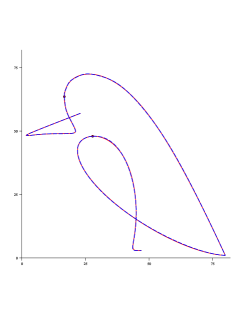
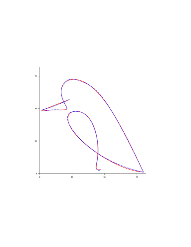
Example 5.1 [Starling‘s sketch] We consider the curve shown in Figure 1 (solid and red), obtained by joining two rational Bézier curves of degree eight each; we say that the composite curve has degree (8,8). The first curve is defined by the control points $(23,57)$, $(-13,43)$, $(29,58)$, $(44,48)$, $(30,42)$, $(13,44)$, $(-2,77)$, $(42,83)$, $(80,1)$, and the associated weights $1,\,4,\,3,\,1,\,5,\,4,\,7,\,6,\,1$, while the second one by $(80,1)$, $(14,4)$, $(3,54)$, $(42,54)$, $(51,42)$, $(36,49)$, $(66,12)$, $(36,2)$, $(47,3)$, and $1,\,1,\,4,\,4,\,2,\,3,\,3,\,7,\,8$. The polynomial composite curve approximation of the above curve with $\alpha=\beta=\frac{1}{2}$, constraints of $C^{1}$- and $C^{2}$-continuity, without and with subdivision, is shown in Figure 1.

Figure 1. Left: Bézier composite curve approximation (dashed and blue) of degree (13,8) to the rational composite Bézier curve (solid and red) of degree (8,8) with the end-point interpolation ($k=l=1$). The errors are $e_{\infty}=\{3.152,\,2.814\}$ and $e_{2}(\frac{1}{2},\frac{1}{2})=\{0.166,\,0.284\}$, respectively. Right: Bézier composite curve approximation (dashed and blue) of degree (12,11,7,6) to the same rational composite Bézier curve (solid and red) of degree (8,8), with one subdivision of each of its two parts, and the end-point derivative interpolation ($k=l=2$). The errors are $e_{\infty}=\{0.559,\,0.811,\,0.146,\,0.231\}$ and $e_{2}(\frac{1}{2},\frac{1}{2})=\{0.063,\,0.104,\,0.045,\,0.081\}$, respectively.

∎

In Examples 5 and 5, we compared our approach with the recently published methods of Huang et al. [7] and Lu [17]. The idea of the first method is the following. Given the rational curve (3.1), use degree elevation to obtain

$$R_{n}(t)=\frac{\displaystyle\sum_{i=0}^{n+h}\omega^{<h>}_{i}r^{<h>}_{i}\,B^{n+h}_{i}(t)}{\displaystyle\sum_{i=0}^{n+h}\omega^{<h>}_{i}\,B^{n+h}_{i}(t)}\qquad(h=0,1,\ldots),$$

and define the sequence of polynomial curves

$$U_{n+h}(t):=\sum_{i=0}^{n+h}r^{<h>}_{i}\,B^{n+h}_{i}(t)\qquad(h=0,1,\ldots).$$

Then $\frac{\mbox{${\rm\,d}$}^{j}}{\mbox{$\mbox{${\rm\,d}$}t$}^{j}}U_{n+h}$ converges uniformly to $\frac{\mbox{${\rm\,d}$}^{j}}{\mbox{$\mbox{${\rm\,d}$}t$}^{j}}R_{n}$ as $h\to\infty$, for any integer $j\geq 0$. The weakness of this approach is that the convergence may be rather slow. Also, notice the increasing degree of the approximating curves.

In the iterative method of Lu [17], the sequence of Bézier curves $\{V^{h}_{n}\}$ is constructed,

$$V^{h}_{n}(t)=\sum_{i=0}^{n}v^{h}_{i}\,B^{n}_{i}(t)\qquad(h=0,1,\ldots),$$

where

$$v^{0}_{i}=R_{n}(t_{i})\qquad(i=0,1,\ldots,n),$$

with $0=t_{0}<t_{1}<\ldots<t_{n}=1$, and

$$v^{h+1}_{i}=v^{h}_{i}+\lambda\left(v^{0}_{i}-V^{h}_{n}(t_{i})\right)\qquad(i=0,1,\ldots,n;\;h=0,1,\ldots),$$

$\lambda$ being a parameter. It is shown that

$$\lim_{h\to\infty}V^{h}_{n}(t_{i})=R_{n}(t_{i})\qquad(i=0,1,\ldots,n).$$

Also this process may be slow, even for carefully chosen factor $\lambda$ (cf. [16]). Another drawback of both methods is that only the simplest constraints (corresponding to $k=l=1$) are accepted.

In the next two examples we let $\alpha=\beta=0$.

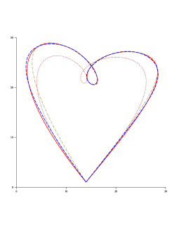
Example 5.2 Our second test rational curve, which has the control points $(14,1)$, $(34,25)$, $(40,38)$, $(-12,24)$, $(5,21)$, $(26,7)$, $(18,41)$, $(-13,34)$, $(14,1)$ and the associated weights $1,\,3,\,3,\,4,\,1,\,7,\,5,$ $3,\,1$, is shown in left part of Figure 2 (solid and red). We compared our approach with the methods of Huang et al. and Lu. We produced polynomial approximation of degree $m=10$ with end-point interpolation constraints (in our method we put $k=l=1$). The results are shown in the left part of Figure 2. Table 2 below lists the errors of approximation in each case (with the number iter of iterations performed in the method of [17]). We see that the method of Huang et al., which is very simple and fast, gives much worse results than two other methods. The convergence of the method of Lu is slow: the result obtained after 100 iterations is 4 times less adequate than ours; also, the comparison of the execution times shows the advantage of our algorithm.

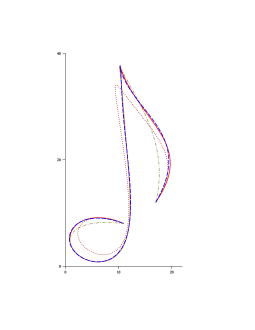
Figure 2. Polynomial approximation of degree 10 to the rational Bézier curve (solid and red) of degree 8 (left) and 9 (right), with end-point interpolation ($k=l=1$). Comparison of the present method (dashed and blue), Huang et al. method (dotted and brown) and Lu method ($100th$ iterate; dotted-dashed and khaki).

Table 2. Errors in the polynomial approximations to the rational Bézier curve, with end-point interpolation

$$\begin{array}[]{lrllr|rllr}&\lx@intercol\hfil\sf Example\leavevmode\nobreak\ \ref{Ex:2}\hfil\lx@intercol&\vrule\lx@intercol\hfil\sf Example\leavevmode\nobreak\ \ref{Ex:3}\hfil\lx@intercol\\ &iter&e_{\infty}&\!\!e_{2}(0,0)&time[s]&iter&e_{\infty}&\!\!e_{2}(0,0)&time[s]\\[1.93748pt] \hline\cr\text{\sf Present method}&\--&0.664&0.167&0.15&\--&0.398&0.106&0.15\\[3.87498pt] \hline\cr\text{\sf Huang {et al.} \cite[cite]{[\@@bibref{}{HSL08}{}{}]}}&\--&9.41&3.98&<0.01&\--&5.78&3.03&<0.01\\[3.87498pt] \hline\cr&25&3.43&0.850&0.18&25&2.82&0.653&0.20\\ \text{\sf Lu \cite[cite]{[\@@bibref{}{Lu11}{}{}]}}&50&2.99&0.729&0.35&50&2.55&0.584&0.37\\ &75&2.79&0.671&0.50&75&2.42&0.550&0.54\\ &100&2.67&0.636&0.67&100&2.34&0.529&0.73\end{array}$$

∎

Example 5.3 $(17,12)$, $(32,34)$, $(-23,24)$, $(33,62)$, $(-23,15)$, $(25,3)$, $(30,-2)$, $(-5,-8)$, $(-5,15)$, $(11,8)$, and the associated weights $1,\,2,\,3,\,6$, $4,\,5,\,3,\,4,\,2,\,1$, is shown in the right part of Figure 2 (solid and red). We produced polynomial approximation of degree $m=10$ with end-point interpolation constraints. The results are shown in the right part of Figure 2 and in Table 2. Again, we see that the methods of Huang et al. and Lu give much less adequate results than our method. ∎

Conclusions

We present a method to solve the constrained least squares approximation of the rational Bézier curve by the Bézier curve. Important tools used are efficient evaluation of the Bézier coefficients of the constrained dual Bernstein basis polynomials associated with the Jacobi scalar product and numerical computation of some integrals involving rational functions. The new algorithm is particularly attractive when it is combined with the subdivision process.

References

• [1] Ahn, Y.J.: Using Jacobi polynomials for degree reduction of Bézier curves with Cksuperscript𝐶𝑘C^{k}-constraints. Comput. Aided Geom. Design 20, 423–434 (2003)
• [2] Cai, H.J., Wang, G.J.: Constrained approximation of rational Bézier curves based on a matrix expression of its end points continuity condition. Comput. Aided Design 42, 495–504 (2010)
• [3] G. Dahlquist, A. Björck, Numerical Methods in Scientific Computing, Vol. I, SIAM, 2008.
• [4] G. E. Farin, Curves and Surfaces for Computer-Aided Geometric Design. A Practical Guide, third ed., Academic Press, Boston, 1996.
• [5] M.S. Floater, High order approximation of rational curves by polynomial curves, Comput. Aided Design 23 (2006) 621–628.
• [6] W.M. Gentleman, Implementing Clenshaw-Curtis quadrature. I and II, Comm. ACM 15 (1972) 337–346.
• [7] Y. Huang, H. Su, H. Lin, A simple method for approximating rational Bézier curve using Bézier curves, Comput. Aided Geom. Design 25 (2008) 697–699.
• [8] P. Keller, A method for indefinite integration of oscillatory and singular functions, Numer. Algor. 46 (2007) 219–251.
• [9] R. Koekoek, P. Lesky, R. F. Swarttouw, Hypergeometric Orthogonal Polynomials and Their q𝑞q-Analogues, Springer, Berlin, 2010.
• [10] B.-G. Lee, Y. Park, Approximate conversion of rational Bézier curves, J. KSIAM 2 (1998) 88–93.
• [11] S. Lewanowicz, Quick construction of recurrence relations for the Jacobi coefficients, J. Comput. Appl. Math. 43 (1992) 355-372.
• [12] S. Lewanowicz, P. Woźny, Multi-degree reduction of tensor product Bézier surfaces with general constraints, Appl. Math. Comput. 217 (2011), 4596-4611.
• [13] S. Lewanowicz, P. Woźny, Bézier representation of the constrained dual Bernstein polynomials, Applied Mathematics and Computation 218 (2011), 4580–4586.
• [14] S. Lewanowicz, P. Woźny, P. Keller, Polynomial approximation of rational Bézier curves with constraints, Numer. Algor. 59 (2012) 607–622.
• [15] L.G. Liu, G.J. Wang, Recursive formulae for Hermite polynomial approximation to rational Bézier curves, in: R. Martin, W.P. Wang (Eds.), Proc. Geom. Modeling and Processing 2000: Theory and Applications, IEEE Computer Soc., Los Alamitos, 2000, pp. 190–197.
• [16] L. Lu, Weighted progressive iteration approximation of rational curves, Comput. Aided Geom. Design 27 (2010) 127–137.
• [17] L. Lu, Sample-based polynomial approximation of rational Bézier curves, J. Comput. Appl. Math. 235 (2011) 1557–1563.
• [18] T.W. Sederberg, M. Kakimoto, Approximating rational curves using polynomial curves, in: G. Farin (Ed.), NURBS for Curve and Surface Design, SIAM, Philadelphia, 1991, pp. 144–158.
• [19] G.J. Wang, T.W. Sederberg, F.L. Chen, On the convergence of polynomial approximation of rational functions, J. Approx. Theory 89 (1997) 267–288.
• [20] P. Woźny, S. Lewanowicz, Multi-degree reduction of Bézier curves with constraints, using dual Bernstein basis polynomials, Comput. Aided Geom. Design 26 (2009) 566–579.