The QC Relaxation: A Theoretical and Computational Study on Optimal Power Flow

Abstract

Convex relaxations of the power flow equations and, in particular, the Semi-Definite Programming (SDP) and Second-Order Cone (SOC) relaxations, have attracted significant interest in recent years. The Quadratic Convex (QC) relaxation is a departure from these relaxations in the sense that it imposes constraints to preserve stronger links between the voltage variables through convex envelopes of the polar representation. This paper is a systematic study of the QC relaxation for AC Optimal Power Flow with realistic side constraints. The main theoretical result shows that the QC relaxation is stronger than the SOC relaxation and neither dominates nor is dominated by the SDP relaxation. In addition, comprehensive computational results show that the QC relaxation may produce significant improvements in accuracy over the SOC relaxation at a reasonable computational cost, especially for networks with tight bounds on phase angle differences. The QC and SOC relaxations are also shown to be significantly faster and reliable compared to the SDP relaxation given the current state of the respective solvers.

Nomenclature

$N$

- The set of nodes in the network

$E$

- The set of from edges in the network

$E^{R}$

- The set of to edges in the network

$\bm{i}$

- imaginary number constant

$I$

- AC current

$S=p+\bm{i}q$

- AC power

$V=v\angle\theta$

- AC voltage

$Z=r+\bm{i}x$

- Line impedance

$Y=g+\bm{i}b$

- Line admittance

$T=t\angle\theta^{t}$

- Transformer properties

$Y^{s}=g^{s}+\bm{i}b^{s}$

- Bus shunt admittance

$W$

- Product of two AC voltages

$l$

- Current magnitude squared, $|I|^{2}$

$b^{c}$

- Line charging

$s^{u}$

- Line apparent power thermal limit

$\theta^{\Delta}$

- Phase angle difference limit

$S^{d}=p^{d}+\bm{i}q^{d}$

- AC power demand

$S^{g}=p^{g}+\bm{i}q^{g}$

- AC power generation

$c_{0},c_{1},c_{2}$

- Generation cost coefficients

$\Re(\cdot)$

- Real part of a complex number

$\Im(\cdot)$

- Imaginary part of a complex number

$(\cdot)^{*}$

- Conjugate of a complex number

$|\cdot|$

- Magnitude of a complex number, $l^{2}$-norm

$x^{l},x^{u}$

- Lower and upper bounds of $x$, respectively

$\widecheck{x}$

- Convex envelope of $x$

$\bm{x}$

- A constant value

I Introduction

Convex relaxations of the power flow equations have attracted significant interest in recent years. They include the Semi-Definite Programming (SDP) [1], Second-Order Cone (SOC) [2], Convex-DistFlow (CDF) [3], and the recent Quadratic Convex (QC) [4] and Moment-Based [5, 6] relaxations. Much of the excitement underlying this line of research comes from the fact that the SDP relaxation has shown to be tight on a variety of case studies [7], opening a new avenue for accurate, reliable, and efficient solutions to a variety of power system applications. Indeed, industrial-strength optimization tools (e.g., Gurobi, cplex, Mosek) are now available to solve various classes of convex optimization problems.

The relationships between the SDP, SOC, and CDF relaxations is now largely well-understood: See [8, 9] for a comprehensive overview. In particular, the SOC and CDF relaxations are known to be equivalent and the SDP relaxation is at least as strong than both of these. However, little is known about the QC relaxation which is a significant departure from these more traditional relaxations. Indeed, one of the key features of the QC relaxation is to compute convex envelopes of the polar representation of the power flow equations in the hope of preserving stronger links between the voltage variables. This contrasts with the SDP and SOC relaxations which are derived from a lift-and-project approach on the complex representation.

This paper fills this gap and provides a theoretical study of the QC relaxation as well as a comprehensive computational evaluation to compare the strengths and weaknesses of these relaxations. Our main contributions can be summarized as follows:

1. The QC relaxation is stronger than the SOC relaxation.

2. The QC relaxation neither dominates nor is dominated by the SDP relaxation.

3. Computational results on optimal power flow show that the QC relaxation may bring significant benefits in accuracy over the SOC relaxation, especially for tight bounds on phase angle differences, for a reasonable loss in efficiency.

4. The computational results also show that, with existing solvers, the SOC and QC relaxations are significantly faster and more reliable than the SDP relaxation.

The theoretical results are derived using the equivalence of two classes of second-order cone constraints (in conjunction with the power equations), which provides an alternative formulation for the QC model which is interesting in its own right. Moreover, to the best of our knowledge, the computational results also represent the most comprehensive comparison of these convex relaxations. They are obtained for optimal power flow problems with realistic side-constraints, featuring bus shunts, line charging, and transformers.

The rest of the paper is organized as follows. Section II reviews the formulation of the AC-OPF problem from first principles and presents two equivalent formulations of this non-convex optimization problem. Section III derives the SDP, QC, and SOC relaxations. Section IV illustrates their behavior on a well-known 3-bus example. Section V presents an alternative formulation of the QC relaxation which is a convenient tool for subsequent proofs. Section VI presents the theoretical results linking the QC to the other relaxations. Section VII reports the computational results for the three relaxations on 93 AC-OPF test cases, and Section VIII concludes the paper.

II AC Optimal Power Flow

This section reviews the specification of AC Optimal Power Flow (AC-OPF) and introduces the notations used in the paper. In the equations, constants are always in bold face. The AC power flow equations are based on complex quantities for current $I$, voltage $V$, admittance $Y$, and power $S$, which are linked by the physical properties of Kirchhoff’s Current Law (KCL), i.e.,

$$I^{g}_{i}-{\bm{I}^{d}_{i}}=\sum_{\begin{subarray}{c}(i,j)\in E\cup E^{R}\end{subarray}}I_{ij}$$ (1)

Ohm’s Law, i.e.,

$$I_{ij}=\bm{Y}_{ij}(V_{i}-V_{j})$$ (2)

and the definition of AC power, i.e.,

$$S_{ij}=V_{i}I_{ij}^{*}$$ (3)

Combining these three properties yields the AC Power Flow equations, i.e.,

$$S^{g}_{i}-{\bm{S}^{d}_{i}}=\sum_{\begin{subarray}{c}(i,j)\in E\cup E^{R}\end{subarray}}S_{ij}\;\;\forall i\in N$$ (4a)

$$S_{ij}=\bm{Y}^{*}_{ij}V_{i}V^{*}_{i}-\bm{Y}^{*}_{ij}V_{i}V^{*}_{j}\;\;(i,j)\in E\cup E^{R}$$ (4b)

These non-convex nonlinear equations define how power flows in the network and are a core building block in many power system applications. However, practical applications typically include various operational side constraints on the power flow. We now review some of the most significant ones.

Generator Capabilities

AC generators have limitations on the amount of active and reactive power they can produce $S^{g}$, which is characterized by a generation capability curve [10]. Such curves typically define nonlinear convex regions which are typically approximated by boxes in AC transmission system test cases, i.e.,

$$\bm{S^{gl}}_{i}\leq S^{g}_{i}\leq\bm{S^{gu}}_{i}\;\;\forall i\in N$$ (5a)

Line Thermal Limit

AC power lines have thermal limits [10] to prevent lines from sagging and automatic protection devices from activating. These limits are typically given in Volt Amp units and constrain the apparent power flows on the lines, i.e.,

$$|S_{ij}|\leq\bm{s^{u}}_{ij}\;\;\forall(i,j)\in E\cup E^{R}$$ (6)

Bus Voltage Limits

Voltages in AC power systems should not vary too far (typically $\pm 10\%$) from some nominal base value [10]. This is accomplished by putting bounds on the voltage magnitudes, i.e.,

$$\bm{v^{l}}_{i}\leq|V_{i}|\leq\bm{v^{u}}_{i}\;\;\forall i\in N$$ (7)

A variety of power flow formulations only have variables for the square of the voltage magnitude, i.e., $|V_{i}|^{2}$. In such cases, the voltage bound constrains can be incorporated via the following constraints:

$$(\bm{v^{l}}_{i})^{2}\leq|V_{i}|^{2}\leq(\bm{v^{u}}_{i})^{2}\;\;\forall i\in N$$ (8)

Phase Angle Differences

Small phase angle differences are also a design imperative in AC power systems [10] and it has been suggested that phase angle differences are typically less than $10$ degrees in practice [11]. These constraints have not typically been incorporated in AC transmission test cases [12]. However, recent work [13, 4] have observed that incorporating Phase Angle Difference (PAD) constraints, i.e.,

$$-\bm{\theta^{\Delta}}_{ij}\leq\angle\!\left(V_{i}V^{*}_{j}\right)\leq\bm{\theta^{\Delta}}_{ij}\;\;\forall(i,j)\in E$$ (9)

is useful in the convexification of the AC power flow equations. For simplicity, this paper assumes that the phase angle difference bounds are symmetrical and within the range $(-\pi/2,\pi/2)$, i.e.,

$$0\leq\bm{\theta^{\Delta}}_{ij}\leq\frac{\pi}{2}\;\;(i,j)\in E$$ (10)

but the results presented here can be extended to more general cases. Observe also that the PAD constraints (9) can be implemented as a linear relation of the real and imaginary components of $V_{i}V^{*}_{j}$ [14], i.e. $\forall(i,j)\in E$,

$$\tan(-\bm{\theta^{\Delta}}_{ij})\Re\left(V_{i}V^{*}_{j}\right)\!\leq\!\Im\left(V_{i}V^{*}_{j}\right)\!\leq\!\tan(\bm{\theta^{\Delta}}_{ij})\Re\left(V_{i}V^{*}_{j}\right)$$ (11)

The usefulness of this formulation will be apparent later in the paper.

Other Constraints

Other line flow constraints have been proposed, such as, active power limits and voltage difference limits [7, 14]. However, we do not consider them here since, to the best of our knowledge, test cases incorporating these constraints are not readily available.

Objective Functions

The last component in formulating OPF problems is an objective function. The two classic objective functions are line loss minimization, i.e.,

$$\mbox{minimize: }\sum_{i\in N}\Re(S^{g}_{i})$$ (12)

and generator fuel cost minimization, i.e.,

$$\mbox{minimize: }\sum_{i\in N}\bm{c}_{2i}(\Re(S^{g}_{i}))^{2}+\bm{c}_{1i}\Re(S^{g}_{i})+\bm{c}_{0i}$$ (13)

Observe that objective (12) is a special case of objective (13) where $\bm{c}_{2i}\!=\!0,\bm{c}_{1i}\!=\!1,\bm{c}_{0i}\!=\!0\;\;(i\!\in\!N)$ [15]. Hence, the rest of this paper focuses on objective (13).

AC-OPF

Combining the AC power flow equations, the side constraints, and the objective function, yields the well-known AC-OPF formulation presented in Model 1. Observe that, in Model 1, the non-convexities arises solely from the product of the voltages (i.e., $V_{i}V_{j}^{*}$) and they can be isolated by introducing new $W$ variables to represent the products of $V$s [16, 2, 17, 18], i.e,

$$V_{i}V_{j}^{*}=W_{ij}\;\;(i,j\in N).$$ (14)

Model 2 presents an equivalent version of the AC-OPF, where the $W$ factorization has been incorporated and the only source of non-convexity is in constraint (16b). Note that this section has introduced the simplest form of the AC-OPF problem and that real-world applications feature a variety of extensions as discussed at length in [19, 20]. In practice, this non-convex nonlinear optimization problem is typically solved with numerical methods (e.g. IPM, SLP) [21, 22], which provide locally optimal solutions if they converge to a feasible point.

Model 1 AC-OPF

variables: $$S^{g}_{i}(\forall i\in N),\;V_{i}(\forall i\in N)$$

minimize: $$\sum_{i\in N}\bm{c}_{2i}(\Re(S^{g}_{i}))^{2}+\bm{c}_{1i}\Re(S^{g}_{i})+\bm{c}_{0i}$$ (15a)

subject to:

$$\bm{v^{l}}_{i}\leq|V_{i}|\leq\bm{v^{u}}_{i}\;\;\forall i\in N$$ (15b)

$$\bm{S^{gl}}_{i}\leq S^{g}_{i}\leq\bm{S^{gu}}_{i}\;\;\forall i\in N$$ (15c)

$$|S_{ij}|\leq\bm{s^{u}}_{ij}\;\;\forall(i,j)\in E\cup E^{R}$$ (15d)

$$S^{g}_{i}-{\bm{S}^{d}_{i}}=\sum_{\begin{subarray}{c}(i,j)\in E\cup E^{R}\end{subarray}}S_{ij}\;\;\forall i\in N$$ (15e)

$$S_{ij}=\bm{Y}^{*}_{ij}V_{i}V^{*}_{i}-\bm{Y}^{*}_{ij}V_{i}V^{*}_{j}\;\;(i,j)\in E\cup E^{R}$$ (15f)

$$-\bm{\theta^{\Delta}}_{ij}\leq\angle(V_{i}V^{*}_{j})\leq\bm{\theta^{\Delta}}_{ij}\;\;\forall(i,j)\in E$$ (15g)

Model 2 AC-OPF-W

$$\mbox{\bf variables: }S^{g}_{i}(\forall i\in N),\;V_{i}(\forall i\in N),\;W_{ij}(\forall i,j\in N)\phantom{123}$$

$$\mbox{\bf minimize: }\sum_{i\in N}\bm{c}_{2i}(\Re(S^{g}_{i}))^{2}+\bm{c}_{1i}\Re(S^{g}_{i})+\bm{c}_{0i}$$ (16a)

subject to:

$$W_{ij}=V_{i}V_{j}^{*}\;\;\forall i\in N,\forall j\in N$$ (16b)

$$(\bm{v^{l}}_{i})^{2}\leq W_{ii}\leq(\bm{v^{u}}_{i})^{2}\;\;\forall i\in N$$ (16c)

$$\bm{S^{gl}}_{i}\leq S^{g}_{i}\leq\bm{S^{gu}}_{i}\;\;\forall i\in N$$ (16d)

$$S^{g}_{i}-{\bm{S}^{d}_{i}}=\sum_{\begin{subarray}{c}(i,j)\in E\cup E^{R}\end{subarray}}S_{ij}\;\;\forall i\in N$$ (16e)

$$S_{ij}=\bm{Y}^{*}_{ij}W_{ii}-\bm{Y}^{*}_{ij}W_{ij}\;\;(i,j)\in E$$ (16f)

$$S_{ji}=\bm{Y}^{*}_{ij}W_{jj}-\bm{Y}^{*}_{ij}W_{ij}^{*}\;\;(i,j)\in E$$ (16g)

$$|S_{ij}|\leq(\bm{s^{u}}_{ij})\;\;\forall(i,j)\in E\cup E^{R}$$ (16h)

$$\tan(-\bm{\theta^{\Delta}}_{ij})\Re(W_{ij})\leq\Im(W_{ij})\leq\tan(\bm{\theta^{\Delta}}_{ij})\Re(W_{ij})$$ (16i)

$$\hskip 156.49014pt\forall(i,j)\in E$$

III Convex Relaxations of Optimal Power Flow

Since the AC-OPF problem is NP-Hard [23, 24] and numerical methods provide limited guarantees for determining feasibility and global optimally, significant attention has been devoted to finding convex relaxations of Model 1. Such relaxations are appealing because they are computationally efficient and may be used to:

1. bound the quality of AC-OPF solutions produced by locally optimal methods;

2. prove that a particular AC-OPF problem has no solution;

3. produce a solution that is feasible in the original non-convex problem [7], thus solving the AC-OPF and guaranteeing that the solution is globally optimal.

The ability to provide bounds is particularly important for the numerous mixed-integer nonlinear optimization problems that arise in power system applications. For these reasons, a variety of convex relaxations of the AC-OPF have been developed including, the SDP [1], QC [4], SOC [2], and Convex-DistFlow [3], which are reviewed in detail in this section. Moreover, since the SOC and Convex-DistFlow relaxations have been shown to be equivalent [25], this paper focuses on the SDP, SOC, and QC relaxations only and shows how they are derived from Model 2. The key insight is that each relaxation presents a different approach to convexifing constraints (16b), which are the only source of non-convexity in Model 2.

The Semi-Definite Programming (SDP) Relaxation

exploits the fact that the $W$ variables are defined by $V(V^{*})^{T}$, which ensures that $W$ is positive semi-definite (denoted by $W\succeq 0$) and has rank 1 [1, 7, 18]. These conditions are sufficient to enforce constraints (16b) [26], i.e.,

$$W_{ij}=V_{i}V_{j}^{*}\;(i,j\in N)\;\;\Leftrightarrow\;\;W\succeq 0\;\wedge\;\mbox{rank}(W)=1$$

The SDP relaxation [27, 26] then drops the rank constraint to obtain Model 3.

Model 3 The SDP Relaxation AC-OPF-W-SDP.

variables: $$S^{g}_{i}(\forall i\in N),\;W_{ij}(\forall i,j\in N)$$

minimize: $$\eqref{w_obj}$$

subject to: (16c)–(16i)

$$W\succeq 0$$ (17a)

Model 4 The SOC Relaxation AC-OPF-W-SOC.

variables: $$S^{g}_{i}(\forall i\in N),\;W_{ij}(\forall(i,j)\in E),\;W_{ii}(\forall i\in N):real$$

minimize: $$\eqref{w_obj}$$

subject to: (16c)–(16i)

$$|W_{ij}|^{2}\leq W_{ii}W_{jj}\;\;\forall(i,j)\in E$$ (18a)

The Second Order Cone (SOC) Relaxation

convexifies each constraint of (16b) separately, instead of considering them globally as in the SDP relaxation. The SOC relaxation takes the absolute square of each constraint, refactors it, and then relaxes the equality into an inequality, i.e.,

$$W_{ij}=V_{i}V^{*}_{j}$$ (19a)

$$W_{ij}W^{*}_{ij}=V_{i}V^{*}_{j}V^{*}_{i}V_{j}$$ (19b)

$$|W_{ij}|^{2}=W_{ii}W_{jj}$$ (19c)

$$|W_{ij}|^{2}\leq W_{ii}W_{jj}$$ (19d)

Equation (19d) is a rotated second-order cone constraint which is widely supported by industrial optimization tools. It can, in fact, be rewritten in the standard form of a second-order cone constraint as,

$$\left|\begin{pmatrix}2W_{ij}\\ W_{ii}-W_{jj}\\ \end{pmatrix}\right|\leq W_{ii}+W_{jj}$$ (20)

The complete SOC formulation is presented in Model 4. Note that this relaxation requires fewer $W$ variables than Model 3. Due to the sparsity of AC power networks, this size reduction can lead to significant memory and computational savings.

The Quadratic Convex (QC) Relaxation

was introduced to preserve stronger links between the voltage variables [4]. It represents the voltages in polar form (i.e., $V=v\angle\theta$) and links these real variables to the $W$ variables, along the lines of [16, 17, 28, 29], using the following equations:

$$W_{ii}=v_{i}^{2}\;\;i\in N$$ (21a)

$$\Re(W_{ij})=v_{i}v_{j}\cos(\theta_{i}-\theta_{j})\;\;\forall(i,j)\in E$$ (21b)

$$\Im(W_{ij})=v_{i}v_{j}\sin(\theta_{i}-\theta_{j})\;\;\forall(i,j)\in E$$ (21c)

The QC relaxation then relaxes these equations by taking tight convex envelopes of their nonlinear terms, exploiting the operational limits for $v_{i},v_{j},\theta_{i}-\theta_{j}$. The convex envelopes for the square and product of variables are well-known [30], i.e.,

$$\langle x^{2}\rangle^{T}\equiv\begin{cases*}\widecheck{x}\geq x^{2}\\ \widecheck{x}\leq(\bm{x^{u}}+\bm{x^{l}})x-\bm{x^{u}}\bm{x^{l}}\end{cases*}$$ (T-CONV)

$$\langle xy\rangle^{M}\equiv\begin{cases*}\widecheck{xy}\geq\bm{x^{l}}y+\bm{y^{l}}x-\bm{x^{l}}\bm{y^{l}}\\ \widecheck{xy}\geq\bm{x^{u}}y+\bm{y^{u}}x-\bm{x^{u}}\bm{y^{u}}\\ \widecheck{xy}\leq\bm{x^{l}}y+\bm{y^{u}}x-\bm{x^{l}}\bm{y^{u}}\\ \widecheck{xy}\leq\bm{x^{u}}y+\bm{y^{l}}x-\bm{x^{u}}\bm{y^{l}}\end{cases*}$$ (M-CONV)

Under our assumptions that the phase angle bound satisfies $0\leq\bm{\theta^{\Delta}}\leq\frac{\pi}{2}$ and is symmetric, convex envelopes for sine (S-CONV) and cosine (C-CONV) [4] are given by,

$$\langle\sin(x)\rangle^{S}\equiv\begin{cases*}\widecheck{sx}\leq\cos\left(\frac{\bm{x^{u}}}{2}\right)\left(x-\frac{\bm{x^{u}}}{2}\right)+\sin\left(\frac{\bm{x^{u}}}{2}\right)\\ \widecheck{sx}\geq\cos\left(\frac{\bm{x^{u}}}{2}\right)\left(x+\frac{\bm{x^{u}}}{2}\right)-\sin\left(\frac{\bm{x^{u}}}{2}\right)\end{cases*}$$

$$\langle\cos(x)\rangle^{C}\equiv\begin{cases*}\widecheck{cx}\leq 1-\frac{1-\cos({\bm{x^{u}}})}{({\bm{x^{u}}})^{2}}x^{2}\\ \widecheck{cx}\geq\cos(\bm{x^{u}})\end{cases*}$$

In the following, we abuse notation and also use $\langle f(\cdot)\rangle^{C}$ to denote the variable on the left-hand side of the convex envelope $C$ for function $f(\cdot)$. When such an expression is used inside an equation, the constraints $\langle f(\cdot)\rangle^{C}$ are also added to the model.

Model 5 The QC Relaxation AC-OPF-C-QC.

variables: $$S^{g}_{i}(\forall i\in N),\;W_{ij}(\forall(i,j)\in E),\;W_{ii}(\forall i\in N):real$$

$$v_{i}\angle\theta_{i}(\forall i\in N),\;l_{ij}(\forall(i,j)\in E)$$

minimize: $$\eqref{w_obj}$$

subject to: (16c)–(16i)

$$W_{ii}=\langle v_{i}^{2}\rangle^{T}\;\;i\in N$$ (22a)

$$\Re(W_{ij})=\langle\langle v_{i}v_{j}\rangle^{M}\langle\cos(\theta_{i}-\theta_{j})\rangle^{C}\rangle^{M}\;\;\forall(i,j)\in E$$ (22b)

$$\Im(W_{ij})=\langle\langle v_{i}v_{j}\rangle^{M}\langle\sin(\theta_{i}-\theta_{j})\rangle^{S}\rangle^{M}\;\;\forall(i,j)\in E$$ (22c)

$$S_{ij}+S_{ji}=\bm{Z}_{ij}l_{ij}\;\;\forall(i,j)\in E$$ (22d)

$$|S_{ij}|^{2}\leq W_{ii}l_{ij}\;\;\forall(i,j)\in E$$ (22e)

Convex envelopes for equations (21a)–(21c) can be obtained by composing the convex envelopes of the functions for square, sine, cosine, and the product of two variables, i.e.,

$$W_{ii}=\langle v_{i}^{2}\rangle^{T}\;\;i\in N$$ (23a)

$$\Re(W_{ij})=\langle\langle v_{i}v_{j}\rangle^{M}\langle\cos(\theta_{i}-\theta_{j})\rangle^{C}\rangle^{M}\;\;\forall(i,j)\in E$$ (23b)

$$\Im(W_{ij})=\langle\langle v_{i}v_{j}\rangle^{M}\langle\sin(\theta_{i}-\theta_{j})\rangle^{S}\rangle^{M}\;\;\forall(i,j)\in E$$ (23c)

The QC relaxation also proposes to strengthen these convex envelopes with a second-order cone constraint based on the absolute square of line power flow (3), first proposed in [3]. This requires a new variable $l_{ij}$ for each line $(i,j)\in E$ that captures the current magnitude squared on that line. The following constraints are added to link the $l_{ij}$ variables to the existing model variables.

$$S_{ij}+S_{ji}=\bm{Z}_{ij}l_{ij}\;\;\forall(i,j)\in E$$ (24a)

$$|S_{ij}|^{2}\leq W_{ii}l_{ij}\;\;\forall(i,j)\in E$$ (24b)

The complete QC relaxation is presented in Model 5. This model is annotated as C-QC, as the second-order cone constraints use current variables. The motivation for this distinction will become clear in Section V.

IV An Illustrative Example

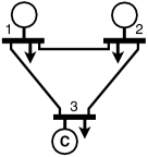
Figure 1: A Network Diagram for the 3-Bus Example.

TABLE I: Three-Bus System Network Data (100 MVA Base).

Bus Parameters
Bus	$\bm{p^{d}}$	$\bm{q^{d}}$	$\bm{v^{l}}$	$\bm{v^{u}}$
1	110	40	0.9	1.1
2	110	40	0.9	1.1
3	95	50	0.9	1.1

Line Parameters
From–To Bus	$\bm{r}$	$\bm{x}$	$\bm{b^{c}}$	$\bm{s^{u}}$	$\bm{\theta^{\Delta}}$
1–2	0.042	0.90	0.30	$\infty$	$30^{\circ}$
2–3	0.025	0.75	0.70	50	$30^{\circ}$
1–3	0.065	0.62	0.45	$\infty$	$30^{\circ}$

Generator Parameters
Generator	$\bm{p^{gl}},\bm{p^{gu}}$	$\bm{q^{gl}},\bm{q^{gu}}$	$\bm{c_{2}}$	$\bm{c_{1}}$	$\bm{c_{0}}$
1	$0,\infty$	$-\infty,\infty$	0.110	5.0	0
2	$0,\infty$	$-\infty,\infty$	0.085	1.2	0
3	$0,0$	$-\infty,\infty$	0	0	0

This section illustrates the three main power flow relaxations on the 3-bus network from [31], which has proven to be an excellent test case for power flow relaxations. This system is depicted in Figure 1 and the associated network parameters are given in Table I. This network is designed to have very few binding constraints. Hence, the generator and line limits are set to large non-binding values, except for the thermal limit constraint on the line between buses 2 and 3, which is set to 50 MVA. In addition to its base configuration, we also consider this network with reduced phase angle difference bounds of $18^{\circ}$. IPOPT [32] is used as a heuristic [33] to find a feasible solution to the AC-OPF and we measure the optimally gap between the heuristic and a relaxation using the formula

$$\frac{\text{Heuristic}-\text{Relaxation}}{\text{Heuristic}}.$$

TABLE II: AC-OPF Bounds using Relaxations on the 3-Bus Case.

	$/h	Optimality Gap (%)
Test Case	AC	SDP	QC	SOC
Base	5812	0.39	1.24	1.32
${\theta^{\Delta}}\!=\!18^{\circ}$	5992	2.06	1.24	4.28

Table II summarizes the results. In the base configuration, the SDP relaxation has the smallest optimality gap. In the ${\theta^{\Delta}}\!=\!18^{\circ}$ case, the QC relaxation has the smallest optimality gap, while reducing the bound on phase angle differences increases the optimality gap for both the SDP and SOC relaxations. This small network highlights two important results. First, the SDP relaxation does not dominate the QC relaxation and vice-versa. Second, the SDP and QC relaxations dominate the SOC relaxation. The next two sections prove that this last result holds for all networks.

V An Alternate Form of the QC Relaxation

Section III introduced two types of second-order cone constraints. Model 4 uses a SOC constraint based on the absolute square of the voltage product [2], i.e.,

$$|W_{ij}|^{2}\leq W_{ii}W_{jj}$$ (25)

while Model 5 uses a SOC constraint based on the absolute square of the power flow [3], i.e.,

$$|S_{ij}|^{2}\leq W_{ii}l_{ij}.$$ (26)

We now show that, in conjunction with the power flow equations (16f)–(16g), these two SOC formulations are equivalent. More precisely, we show that

$$\begin{array}[]{ll}&S_{ij}=\bm{Y}^{*}_{ij}W_{ii}-\bm{Y}^{*}_{ij}W_{ij}\;\;(i,j)\in E\\ &S_{ji}=\bm{Y}^{*}_{ij}W_{jj}-\bm{Y}^{*}_{ij}W_{ij}^{*}\;\;(i,j)\in E\\ &|W_{ij}|^{2}\leq W_{ii}W_{jj}\;\;(i,j)\in E\\ \end{array}$$ (W-SOC)

is equivalent to

$$\begin{array}[]{ll}&S_{ij}=\bm{Y}^{*}_{ij}W_{ii}-\bm{Y}^{*}_{ij}W_{ij}\;\;(i,j)\in E\\ &S_{ji}=\bm{Y}^{*}_{ij}W_{jj}-\bm{Y}^{*}_{ij}W_{ij}^{*}\;\;(i,j)\in E\\ &S_{ij}+S_{ji}=\bm{Z}_{ij}l_{ij}\;\;(i,j)\in E\\ &|S_{ij}|^{2}\leq W_{ii}l_{ij}\;\;(i,j)\in E.\end{array}$$ (C-SOC)

Model 6 The Alternate QC Relaxation AC-OPF-W-QC

variables: $$S^{g}_{i}(\forall i\in N),\;W_{ij}(\forall(i,j)\in E),\;W_{ii}(\forall i\in N):real$$

$$v_{i}\angle\theta_{i}(\forall i\in N)$$

minimize: $$\eqref{w_obj}$$

subject to: (16c)–(16i), (22a)–(22c), (18a)

This equivalence suggests an alternative formulation of the QC relaxation which is given in Model 6 and establishes a clear connection between Models 4 and 5. Throughout this paper, we use $W$ and $C$ to denote which of these equivalent formulations is used.

We now prove these results. The following lemma, whose proof is straight-forward and can be found in the Appendix, establishes some useful equalities.

Lemma V.1.

The following four equalities hold:

1. $|S_{ij}|^{2}=|\bm{Y}_{ij}|^{2}\left(W_{ii}^{2}-W_{ii}W_{ij}-W_{ii}W^{*}_{ij}+|W_{ij}|^{2}\right)$.

2. $|W_{ij}|^{2}=W_{ii}^{2}-W^{*}_{ii}\bm{Z}^{*}_{ij}S_{ij}-W_{ii}\bm{Z}_{ij}S^{*}_{ij}+|\bm{Z}_{ij}|^{2}|S_{ij}|^{2}$.

3. $l_{ij}=|\bm{Y}_{ij}|^{2}(W_{ii}+W_{jj}-W_{ij}-W^{*}_{ij})$.

4. $W_{jj}=W_{ii}-\bm{Z}^{*}_{ij}S_{ij}-\bm{Z}_{ij}S^{*}_{ij}+|\bm{Z}_{ij}|^{2}l_{ij}$.

We are now ready to prove the main result of this section.

Theorem V.2.

(C-SOC) is equivalent to (W-SOC).

Proof.

The proof is similar in spirit to those presented in [25, 34].

W-SOC $\Rightarrow$ C-SOC

Every solution to (W-SOC) is a solution to (C-SOC). Given a solution to (W-SOC), by equality (3) in Lemma V.1, we assign $l_{ij}$ as follows:

$$l_{ij}=|\bm{Y}_{ij}|^{2}(W_{ii}-W_{ij}-W^{*}_{ij}+W_{jj})\;\;(i,j)\in E$$

This assignment satisfies the power loss constraint (22d) by definition of the power. It remains to show that second-order cone constraint in (C-SOC) is satisfied. Using equalities (1) and (3) in Lemma V.1, we obtain

$$|S_{ij}|^{2}=|\bm{Y}_{ij}|^{2}\left(W_{ii}^{2}-W_{ii}W_{ij}-W_{ii}W^{*}_{ij}+|W_{ij}|^{2}\right)$$

$$|S_{ij}|^{2}\leq|\bm{Y}_{ij}|^{2}\left(W_{ii}^{2}-W_{ii}W_{ij}-W_{ii}W^{*}_{ij}+W_{ii}W_{jj}\right)$$

$$|S_{ij}|^{2}\leq W_{ii}|\bm{Y}_{ij}|^{2}\left(W_{ii}-W_{ij}-W^{*}_{ij}+W_{jj}\right)$$

$$|S_{ij}|^{2}\leq W_{ii}l_{ij}.$$

C-SOC $\Rightarrow$ W-SOC

Every solution to (C-SOC) is a solution to (W-SOC). We show that the values of $W_{ij}$ in (C-SOC) satisfy the second-order cone constraint in (W-SOC). Using equalities (2) and (4) in Lemma V.1 and the fact that $W_{ii}=W^{*}_{ii}$ since $W_{ii}$ is a real number, we have

$$|W_{ij}|^{2}=W_{ii}^{2}-W^{*}_{ii}\bm{Z}^{*}_{ij}S_{ij}-W_{ii}\bm{Z}_{ij}S^{*}_{ij}+|\bm{Z}_{ij}|^{2}|S_{ij}|^{2}$$

$$|W_{ij}|^{2}\leq W_{ii}^{2}-W^{*}_{ii}\bm{Z}^{*}_{ij}S_{ij}-W_{ii}\bm{Z}_{ij}S^{*}_{ij}+|\bm{Z}_{ij}|^{2}W_{ii}l_{ij}$$

$$|W_{ij}|^{2}\leq W_{ii}(W_{ii}-\bm{Z}^{*}_{ij}S_{ij}-\bm{Z}_{ij}S^{*}_{ij}+|\bm{Z}_{ij}|^{2}l_{ij})$$

$$|W_{ij}|^{2}\leq W_{ii}W_{jj}$$

and the result follows. ∎

Corollary V.3.

Model 5 is equivalent to Model 6.

Computational results on these two formulations are presented in the Appendix. The main message is that the C-SOC formulation is preferable to W-SOC in the current state of the solving technology, especially on very large networks.

It is important to note that, for clarity, the proofs are presented on the purest version of the AC power flow equations. Transmission system test cases typically include additional parameters such as bus shunts, line charging, and transformers. Proofs that these results can be extended to include the additional parameters in transmission system test cases are presented in the Appendix.

VI Relations of the Power Flow Relaxations

We are now in a position to state the relationships between the convex relaxations. Recall that model $M_{1}$ is a relaxation of model $M_{2}$, denoted by $M_{2}\subseteq M_{1}$, if the solution set of $M_{2}$ is included in the solution set $M_{1}$. We use $M_{1}\neq M_{2}$ to denote the fact that neither $M_{2}\subseteq M_{1}$ nor $M_{1}\subseteq M_{2}$ holds. Since our relaxations have different sets of variables, we define the solution set as the assignments to the $W_{ij}$ variables.

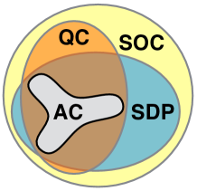
Figure 2: A Venn Diagram of the Solutions Sets for Various AC Power Flow Relaxations (set sizes in this illustration are not to scale).

Theorem VI.1.

The following properties, illustrated in Figure 2, hold:

1. $SDP\subseteq SOC$.

2. $SDP\neq QC$.

3. $QC\subseteq SOC$.

Proof.

Properties (1) and (2) follows from [18] and Section IV respectively. For Property (3), observe that the set of constraints in Model 6 (W-QC) is a superset of those in Model 4. The result follows from Corollary V.3. ∎

Observe that the additional constraints (22a)–(22c) in the QC formulations are parameterized by the $\theta^{\Delta}$. As $\theta^{\Delta}$ grows larger, the QC model reduces to the SOC model. Clearly, the strength of the QC relaxation is sensitive to this input parameter, as illustrated in Section IV.

VII Computational Evaluation

This section presents a computational evaluation of the relaxations and address the following questions:

1. How big are the optimality gaps in practice?

2. What are the runtime requirements of the relaxations?

3. How robust is the solving technology for the relaxations?

The relaxations were compared on 105 state-of-the-art AC-OPF transmission system test cases from the NESTA v0.4.0 archive [35]. These test cases range from as few as 3 buses to as many as 9000 and consist of 35 different networks under a typical operating condition (TYP), a congested operating condition (API), and a small angle difference condition (SAD).

Experimental Setting

All of the computations are conducted on Dell PowerEdge R415 servers with Dual 2.8GHz AMD 6-Core Opteron 4184 CPUs and 64GB of memory. IPOPT 3.12 [32] with linear solver ma27 [36], as suggested by [37], was used as a heuristic for finding locally optimal feasible solutions to the non-convex AC-OPF formulated in AMPL [38]. The SDP relaxation was executed on the state-of-the-art implementation [39] which uses a branch decomposition [40] with a minor extension to add constraint (16i). The SDP solver SDPT3 4.0 [41] was used with the modifications suggested in [39]. The second-order cone models were formulated in AMPL and IPOPT was used to solve the models. Numerical stability appears to be a significant challenge on the power networks with more than 1000 buses [42]. Note that IPOPT is single-threaded and does not take advantage of the multiple cores available in the computation servers. This gives some computational advantage to the SDP solver, which utilizes multiple cores.

Challenging Test Cases

We observe that 52 of the 105 test cases considered have an optimality gap of less than 1.0% with the SOC relaxation. Such test cases are not particularly useful for this study as the improvements of the SDP and QC models are minor. Hence, we focus our attention on the 53 test cases where the SOC optimality gap is greater than 1.0%. The results are displayed in Table III.

TABLE III: Quality and Runtime Results of AC Power Flow Relaxations

	$/h	Optimality Gap (%)				Runtime (seconds)
Test Case	AC	SDP	QC	SOC	CP	AC	SDP	QC	SOC	CP
Typical Operating Conditions (TYP)
nesta_case3_lmbd	5812.64	0.39	1.24	1.32	2.99	0.12	4.16	0.07	0.05	0.03
nesta_case5_pjm	17551.89	5.22	14.54	14.54	15.62	0.04	5.36	0.09	0.03	0.05
nesta_case30_ieee	204.97	0.00	15.64	15.88	27.91	0.09	8.38	0.17	0.07	0.06
nesta_case118_ieee	3718.64	0.06	1.72	2.07	7.87	0.41	12.62	0.87	0.43	0.05
nesta_case162_ieee_dtc	4230.23	1.08	4.00	4.03	15.44	0.61	35.20	1.48	0.31	0.04
nesta_case300_ieee	16891.28	0.08	1.17	1.18	n.a.	0.80	29.69	2.83	0.65	n.a.
nesta_case2224_edin	38127.69	1.22	6.03	6.09	8.45	11.42	690.16	65.59	45.99	0.33
nesta_case2383wp_mp	1868511.78	0.37	1.04	1.05	5.35	12.41	1966.10	57.87	12.91	0.80
nesta_case3012wp_mp	2600842.72	—	1.00	1.02	n.a.	12.40	14588.79†	53.59	19.15	n.a.
nesta_case9241_pegase	315913.26	—	1.67	—	n.a.	132.25	—	3064.42	—	n.a.
Congested Operating Conditions (API)
nesta_case3_lmbd__api	367.74	1.26	1.83	3.30	14.79	0.18	4.41	0.09	0.05	0.23
nesta_case6_ww__api	273.76	0.00⋆	13.14	13.33	17.17	0.34	13.19	0.07	0.06	0.03
nesta_case14_ieee__api	325.56	0.00	1.34	1.34	8.89	0.19	5.64	0.11	0.08	0.94
nesta_case24_ieee_rts__api	6421.37	1.45	13.77	20.70	24.12	0.14	7.50	0.26	0.09	0.04
nesta_case30_as__api	571.13	0.00	4.76	4.76	8.01	0.38	6.12	0.17	0.11	1.11
nesta_case30_fsr__api	372.14	11.06	45.97	45.97	48.80	0.25	7.25	0.19	0.09	0.92
nesta_case30_ieee__api	415.53	0.00	1.01	1.01	12.75	0.07	6.60	0.19	0.09	0.03
nesta_case39_epri__api	7466.25	0.00	2.97	2.99	13.31	0.10	7.36	0.29	0.12	0.04
nesta_case73_ieee_rts__api	20123.98	4.29	12.01	14.34	17.83	0.48	10.03	0.66	0.20	0.06
nesta_case89_pegase__api	4288.02	18.11	20.39	20.43	22.60	1.16	21.58	1.29	0.81	0.04
nesta_case118_ieee__api	10325.27	31.50	43.93	44.08	49.69	0.46	12.59	0.84	0.25	0.05
nesta_case162_ieee_dtc__api	6111.68	0.85	1.33	1.34	19.39	0.50	36.85	1.53	0.39	0.05
nesta_case189_edin__api	1982.82	0.05	5.78	5.78	n.a.	1.07	16.10	1.14	0.33	n.a.
nesta_case2224_edin__api	46235.43	1.10	2.77	2.77	9.07	12.28	672.04	81.66	88.33	0.33
nesta_case2383wp_mp__api	23499.48	0.10	1.12	1.12	3.10	9.50	1421.39	28.37	10.25	0.34
nesta_case2736sp_mp__api	25437.70	0.07	1.32	1.33	3.89	9.21	2278.77	41.29	10.51	0.36
nesta_case2737sop_mp__api	21192.40	0.00	1.05	1.06	4.62	9.29	1887.22	30.94	9.91	0.32
nesta_case2869_pegase__api	96573.10	0.92⋆	1.49	1.49	5.16	21.03	1579.87	102.55	161.96	0.37
nesta_case3120sp_mp__api	22874.98	—	3.02	3.03	n.a.	14.92	15018.93†	41.72	12.19	n.a.
nesta_case9241_pegase__api	241975.18	—	2.45	2.59	n.a.	140.73	—	3511.60	8387.11	n.a.
Small Angle Difference Conditions (SAD)
nesta_case3_lmbd__sad	5992.72	2.06	1.24⋆	4.28	5.90	0.19	4.39	0.10	0.05	0.03
nesta_case4_gs__sad	324.02	0.05	0.81	4.90	66.06	0.24	4.16	0.06	0.06	0.07
nesta_case5_pjm__sad	26423.32	0.00	1.10	3.61	43.95	0.08	5.35	0.11	0.05	0.03
nesta_case6_c__sad	24.43	0.00	0.40	1.36	6.79	0.26	5.32	0.11	0.05	0.02
nesta_case9_wscc__sad	5590.09	0.00	0.41	1.50	6.69	0.14	4.18	0.19	0.05	0.03
nesta_case24_ieee_rts__sad	79804.96	6.05	3.88	11.42	23.56	0.10	6.24	0.30	0.11	0.04
nesta_case29_edin__sad	46933.26	28.44	20.57	34.47	36.79	0.70	9.19	1.73	0.27	0.06
nesta_case30_as__sad	914.44	0.47	3.07	9.16	16.06	0.18	6.49	0.22	0.09	0.03
nesta_case30_ieee__sad	205.11	0.00	3.96	5.84	27.96	0.12	7.49	0.18	0.09	0.03
nesta_case73_ieee_rts__sad	235241.70	4.10	3.51	8.37	22.21	0.30	9.48	0.87	0.20	0.07
nesta_case118_ieee__sad	4324.17	7.57	8.32	12.89	20.77	0.56	14.14	0.98	0.31	0.06
nesta_case162_ieee_dtc__sad	4369.19	3.65	6.91	7.08	18.13	0.81	39.71	1.70	0.36	0.05
nesta_case189_edin__sad	914.61	1.20⋆	2.22	2.25	n.a.	0.65	14.83	1.27	0.46	n.a.
nesta_case300_ieee__sad	16910.23	0.13	1.16	1.26	n.a.	1.01	29.63	2.81	0.76	n.a.
nesta_case2224_edin__sad	38385.14	1.22	5.57	6.18	9.06	11.53	691.53	50.34	65.68	0.33
nesta_case2383wp_mp__sad	1935308.12	1.30	2.97	4.00	8.62	16.25	1785.26	40.71	12.57	0.80
nesta_case2736sp_mp__sad	1337042.77	2.18⋆	2.01	2.34	4.56	13.22	1737.25	35.42	11.31	0.48
nesta_case2737sop_mp__sad	795429.36	2.24⋆	2.21	2.42	3.95	13.01	2153.37	32.05	9.69	0.39
nesta_case2746wp_mp__sad	1672150.46	2.41⋆	1.83	2.44	5.43	14.01	2840.32	35.66	13.32	0.56
nesta_case2746wop_mp__sad	1241955.30	2.71⋆	2.48	2.94	5.14	14.51	2306.18	32.41	23.22	0.42
nesta_case3012wp_mp__sad	2635451.29	—	1.92	2.12	n.a.	15.79	13548.13†	46.59	28.41	n.a.
nesta_case3120sp_mp__sad	2203807.23	—	2.56	2.79	n.a.	30.01	16804.55†	53.81	15.69	n.a.
nesta_case9241_pegase__sad	315932.06	—	0.80	1.75	n.a.	80.30	—	3531.62	33437.86	n.a.

bold - the relaxation provided a feasible AC power flow, $\star$ - solver reported numerical accuracy warnings, —,$\dagger$ - iteration or memory limit

VII-A The Quality of the Relaxations

The first six columns of Table III present the optimality gaps for each of the relaxations on the 53 challenging NESTA test cases. Note that bold values indicate cases where the relaxation produced a solution to the non-convex AC power flow problem. The table illustrates that this is a rare occurrence in the cases considered.

The SDP Relaxation

Overall, the SDP relaxation tends to be the tightest, often featuring optimality gaps below 1.0%. In 5 of the 53 cases, the SDP relaxation even produces a feasible AC power flow solution (as first observed in [7]). However, with six notable cases where the gap is above 5%, it is clear that small gaps are not guaranteed. In some cases, the optimality gap can be as large as 30%.

A significant issue with the SDP relaxation is the reliability of the solving technology. Even after applying the solver modifications suggested in [39], the solver fails to converge to a solution before hitting the default iteration limit on 8 of the 53 test cases shown, it reports numerical accuracy warnings on 4 of the test cases, and ran out of memory on the 3 test cases with more 9000 nodes.

The QC and SOC Relaxations

As suggested by the theoretical study in Section VI, when the phase angle difference bounds are large, the QC relaxation is quite similar to the SOC relaxation. However, when the phase angle difference bounds are tight (e.g., in the SAD cases), the QC relaxation has significant benefits over the SOC relaxation. On average, the SDP relaxation dominates the QC and SOC relaxations. However, there are several notable cases (e.g. nesta_case24_ieee_rts__sad, nesta_case29_edin__sad, nesta_case73_ieee_rts__sad) where the QC relaxation dominates the SDP relaxation.

The Copper Plate (CP) Relaxation

This relaxation indicates the cost of supplying power to the loads when there are no line losses or network constraints [43], and is included in the table as a point of reference. Note that this relaxation cannot be applied to networks containing lines with negative resistance or impedance, as indicated by “n.a.”.

VII-B The Performance of the Relaxations

Detailed runtime results for the heuristic solution method and the relaxations are presented in the last four columns of Table III. The AC heuristic is fast, often taking less than 1 second on test cases with less than 1000 buses. The SOC relaxation most often has very similar performance to the AC heuristic. The additional constraints in the QC relaxation add a factor 2–5 on top of the SOC relaxation. In contrast to these other methods, the SDP relaxation stands out, taking 10–100 times longer. It is interesting to observe, in the 5 cases where the SDP relaxation finds an AC-feasible solution, the heuristic finds a solution of equal quality in a fraction of the time. Focusing on the test cases where the SDP fails to converge, we observe that the failure occurs after several minutes of computation, further emphasizing the reliability issue.

VIII Conclusion

This paper compared the QC relaxation of the power flow equations with the well-understood SDP and SOC relaxations both theoretically and experimentally. Its two main contributions are as follows:

1. The QC relaxation is stronger than the SOC relaxation and neither dominates nor is dominated by the SDP relaxation.

2. Computational results on optimal power flow show that the QC relaxation may bring significant benefits in accuracy over the SOC relaxation, especially for tight bounds on phase angle differences, for a reasonable loss in efficiency. In addition, they show that, with existing solvers, the SOC and QC relaxations are significantly faster and more reliable than the SDP relaxation.

There are two natural frontiers for future work on these relaxations; One is to utilize these relaxations in power system applications that are modeled as mixed-integer nonlinear optimization problems, such as the Optimal Transmission Switching, Unit Commitment, or Transmission Network Expansion Planning. Indeed, Mixed-Integer Quadratic Programming solvers are already being used to extend these relaxations to richer power system applications [4, 44, 45, 46, 47]. The other frontier is to develop novel methods for closing the significant optimality gaps that remain on a variety of test cases considered here.

Carleton Coffrin received a B.Sc. in Computer Science and a B.F.A. in Theatrical Design from the University of Connecticut, Storrs, CT and a M.S. and Ph.D. from Brown University, Providence, RI. He is currently a staff researcher at National ICT Australia where he studies the application of optimization methods to problems in power systems.

Hassan L. Hijazi received a Ph.D. in Computer Science from AIX-Marseille University while working at Orange Labs - France Telecom R&D from 2007 to 2010. He then joined the Optimization Group at the Computer Science Laboratory of the Ecole Polytechnique-France where he stayed until late 2012. He is currently a senior research scientist at National ICT Australia and a senior lecturer at the Australian National University. His main field of research is mixed-integer nonlinear optimization and applications in network-based problems, where he has given contributions both in theory and practice.

Pascal Van Hentenryck received the undergraduate and Ph.D. degrees from the University of Namur, Namur, Belgium. He currently leads the Optimization Research Group at National ICT Australia and holds the Vice-Chancellor Chair in data-intensive computing at the Australian National University, Canberra, Australia. Prior to that, he was a Professor with Brown University, Providence, RI, USA. His current research interests are in optimization with applications to disaster management, power systems, and transportation.

Proof of Lemma V.1

Proof.

 
Property 1 – the absolute square of power –

$$|S_{ij}|^{2}=|\bm{Y}_{ij}|^{2}\left(W_{ii}^{2}-W_{ii}W_{ij}-W_{ii}W^{*}_{ij}+|W_{ij}|^{2}\right)$$

is derived using the following steps:

$$S_{ij}=\bm{Y}^{*}_{ij}W_{ii}-\bm{Y}^{*}_{ij}W_{ij}$$

$$S_{ij}S^{*}_{ij}=(\bm{Y}^{*}_{ij}W_{ii}-\bm{Y}^{*}_{ij}W_{ij})(\bm{Y}_{ij}W^{*}_{ii}-\bm{Y}_{ij}W^{*}_{ij})$$

$$|S_{ij}|^{2}=|\bm{Y}_{ij}|^{2}W_{ii}W^{*}_{ii}-|\bm{Y}_{ij}|^{2}W^{*}_{ii}W_{ij}-|\bm{Y}_{ij}|^{2}W_{ii}W^{*}_{ij}$$

$$+|\bm{Y}_{ij}|^{2}W_{ij}W^{*}_{ij}$$

$$|S_{ij}|^{2}=|\bm{Y}_{ij}|^{2}\left(W_{ii}^{2}-W_{ii}W_{ij}-W_{ii}W^{*}_{ij}+|W_{ij}|^{2}\right).$$

Property 2 – the absolute square of the voltage product –

$$|W_{ij}|^{2}=W_{ii}^{2}-W^{*}_{ii}\bm{Z}^{*}_{ij}S_{ij}-W_{ii}\bm{Z}_{ij}S^{*}_{ij}+|\bm{Z}_{ij}|^{2}|S_{ij}|^{2}$$

is derived using the following steps:

$$S_{ij}=\bm{Y}^{*}_{ij}W_{ii}-\bm{Y}^{*}_{ij}W_{ij}$$

$$W_{ij}=W_{ii}-\bm{Z}^{*}_{ij}S_{ij}$$

$$W_{ij}W^{*}_{ij}=(W_{ii}-\bm{Z}^{*}_{ij}S_{ij})(W^{*}_{ii}-\bm{Z}_{ij}S^{*}_{ij})$$

$$|W_{ij}|^{2}=W_{ii}^{2}-W^{*}_{ii}\bm{Z}^{*}_{ij}S_{ij}-W_{ii}\bm{Z}_{ij}S^{*}_{ij}+|\bm{Z}_{ij}|^{2}|S_{ij}|^{2}.$$

Property 3 – the absolute square of current –

$$l_{ij}=|\bm{Y}_{ij}|^{2}(W_{ii}+W_{jj}-W_{ij}-W^{*}_{ij})$$

is derived using the following steps:

$$I_{ij}=\bm{Y}_{ij}(V_{i}-V_{j})$$

$$I_{ij}I^{*}_{ij}=\bm{Y}_{ij}(V_{i}-V_{j})\bm{Y}^{*}_{ij}(V^{*}_{i}-V^{*}_{j})$$

$$|I_{ij}|^{2}=|\bm{Y}_{ij}|^{2}(V_{i}V^{*}_{i}-V_{i}V^{*}_{j}-V^{*}_{i}V_{j}+V_{j}V^{*}_{j})$$

$$l_{ij}=|\bm{Y}_{ij}|^{2}(W_{ii}-W_{ij}-W^{*}_{ij}+W_{jj}).$$

Property 4 – voltage drop –

$$W_{jj}=W_{ii}-\bm{Z}^{*}_{ij}S_{ij}-\bm{Z}_{ij}S^{*}_{ij}+|\bm{Z}_{ij}|^{2}l_{ij}$$

is derived using the following steps:

$$W_{jj}=W_{jj}$$

$$W_{jj}=W_{ii}-W_{ii}+W_{ij}-W_{ii}+W^{*}_{ij}$$

$$+W_{ii}-W_{ij}-W^{*}_{ij}+W_{jj}$$

$$W_{jj}=W_{ii}-W_{ii}+W_{ij}-W_{ii}+W^{*}_{ij}+|\bm{Z}_{ij}|^{2}l_{ij}$$

$$W_{jj}=W_{ii}-\bm{Z}^{*}_{ij}S_{ij}-\bm{Z}_{ij}S^{*}_{ij}+|\bm{Z}_{ij}|^{2}l_{ij}.$$

Note that property 3 is used in the second step. ∎

Extensions for Transmission System Test Cases

In the interest of clarity, properties of AC Power Flow, and their relaxations, are most often presented on the purest version of the AC power flow equations. However, transmission system test cases include additional parameters such as bus shunts, line charging, and transformers, which complicate the AC power flow equations significantly. Model 7 presents the AC Optimal Power Flow problem (similar to Model 2) with these extensions. In the rest of this section, we show that the results of Section V continue to hold in this extended power flow model.

Model 7 AC-OPF-W with Extensions

variables: $$S^{g}_{i}(\forall i\in N),\;W_{ij}(\forall i,j\in N)$$

minimize: $$\eqref{w_obj}$$ (34a)

subject to: (16b)–(16d), (16h)–(16i)

$$S^{g}_{i}-{\bm{S}^{d}_{i}}-\bm{Y}^{s}_{i}W_{ii}=\sum_{\begin{subarray}{c}(i,j)\in E\cup E^{R}\end{subarray}}S_{ij}\;\;\forall i\in N$$ (34b)

$$S_{ij}=\left(\bm{Y}^{*}_{ij}-\bm{i}\frac{\bm{b^{c}}_{ij}}{2}\right)\frac{W_{ii}}{|\bm{T}_{ij}|^{2}}-\bm{Y}^{*}_{ij}\frac{W_{ij}}{\bm{T}^{*}_{ij}}\;\;(i,j)\in E$$ (34c)

$$S_{ji}=\left(\bm{Y}^{*}_{ij}-\bm{i}\frac{\bm{b^{c}}_{ij}}{2}\right)W_{jj}-\bm{Y}^{*}_{ij}\frac{W^{*}_{ij}}{\bm{T}_{ij}}\;\;(i,j)\in E$$ (34d)

The Two SOC Formulations

In this extended power flow formulation, the second-order cone constraint based on the absolute square of the voltage product [2] remains the same, i.e.,

$$|W_{ij}|^{2}\leq W_{ii}W_{jj}$$ (35)

However, the constraint based on the absolute square of the power flow [3] is updated to include the transformer tap ratio as follows:

$$|S_{ij}|^{2}\leq\frac{W_{ii}}{|\bm{T}_{ij}|^{2}}l_{ij}$$ (36)

and the power loss constraint (22d) is updated to

$$S_{ij}+S_{ji}=\bm{Z}_{ij}\left(l_{ij}+\left(\frac{\bm{b^{c}}_{ij}}{2}\right)^{\!2}\!\frac{W_{ii}}{|\bm{T}_{ij}|^{2}}+\bm{b^{c}}_{ij}\Im(S_{ij})\right)$$

$$-\bm{i}\frac{\bm{b^{c}}_{ij}}{2}\left(\frac{W_{ii}}{|\bm{T}_{ij}|^{2}}+W_{jj}\right)$$ (37)

We now show that, when the power flow equations (34c)–(34d) are present in the model, these two versions of the second-order cone constraints are also equivalent, i.e.,

$$\begin{array}[]{ll}&S_{ij}=\left(\bm{Y}^{*}_{ij}-\bm{i}\frac{\bm{b^{c}}_{ij}}{2}\right)\frac{W_{ii}}{|\bm{T}_{ij}|^{2}}-\bm{Y}^{*}_{ij}\frac{W_{ij}}{\bm{T}^{*}_{ij}}\;\;(i,j)\in E\\ &S_{ji}=\left(\bm{Y}^{*}_{ij}-\bm{i}\frac{\bm{b^{c}}_{ij}}{2}\right)W_{jj}-\bm{Y}^{*}_{ij}\frac{W^{*}_{ij}}{\bm{T}_{ij}}\;\;(i,j)\in E\\ &|W_{ij}|^{2}\leq W_{ii}W_{jj}\;\;(i,j)\in E\\ \end{array}$$ (W-E-SOC)

is equivalent to

$$\begin{array}[]{ll}&S_{ij}=\left(\bm{Y}^{*}_{ij}-\bm{i}\frac{\bm{b^{c}}_{ij}}{2}\right)\frac{W_{ii}}{|\bm{T}_{ij}|^{2}}-\bm{Y}^{*}_{ij}\frac{W_{ij}}{\bm{T}^{*}_{ij}}\;\;(i,j)\in E\\ &S_{ji}=\left(\bm{Y}^{*}_{ij}-\bm{i}\frac{\bm{b^{c}}_{ij}}{2}\right)W_{jj}-\bm{Y}^{*}_{ij}\frac{W^{*}_{ij}}{\bm{T}_{ij}}\;\;(i,j)\in E\\ &S_{ij}+S_{ji}=\bm{Z}_{ij}\left(l_{ij}+\left(\frac{\bm{b^{c}}_{ij}}{2}\right)^{\!2}\!\frac{W_{ii}}{|\bm{T}_{ij}|^{2}}+\bm{b^{c}}_{ij}\Im(S_{ij})\right)\\ &-\bm{i}\frac{\bm{b^{c}}_{ij}}{2}\left(\frac{W_{ii}}{|\bm{T}_{ij}|^{2}}+W_{jj}\right)\;\;(i,j)\in E\\ &|S_{ij}|^{2}\leq\frac{W_{ii}}{|\bm{T}_{ij}|^{2}}l_{ij}\;\;(i,j)\in E.\end{array}$$ (C-E-SOC)

We begin by redeveloping the properties of Lemma V.1 in the extended model.

The Equalities

As both models contain constraints (34c)–(34d), the properties arising from these equations can be transferred between both models.

Proof.

 
Property 1 – the absolute square of power –

$$|S_{ij}|^{2}=|\bm{Y}_{ij}|^{2}\left(\frac{W_{ii}^{2}}{|\bm{T}_{ij}|^{4}}-\frac{W_{ii}}{|\bm{T}_{ij}|^{2}}\frac{W_{ij}}{\bm{T}^{*}_{ij}}-\frac{W_{ii}}{|\bm{T}_{ij}|^{2}}\frac{W^{*}_{ij}}{\bm{T}_{ij}}+\frac{|W_{ij}|^{2}}{|\bm{T}_{ij}|^{2}}\right)$$

$$-\left(\frac{\bm{b^{c}}_{ij}}{2}\right)^{\!2}\!\frac{W_{ii}^{2}}{|\bm{T}_{ij}|^{4}}-\bm{b^{c}}_{ij}\frac{W_{ii}}{|\bm{T}_{ij}|^{2}}\Im(S_{ij})$$ (38)

The derivation follows similarly to the one presented earlier and the details are left to the reader. The only delicate point is to observe that three separate terms in the initial expansion can be collected into $\Im(S_{ij})$.

Property 2 – the absolute square of the voltage product –

$$|W_{ij}|^{2}=(1-\bm{b^{c}}_{ij}\Im(\bm{Z}_{ij}))\frac{W_{ii}^{2}}{|\bm{T}_{ij}|^{2}}-W^{*}_{ii}\bm{Z}^{*}_{ij}S_{ij}-W_{ii}\bm{Z}_{ij}S^{*}_{ij}$$

$$+|\bm{Z}_{ij}|^{2}\left(|\bm{T}_{ij}|^{2}|S_{ij}|^{2}+\left(\frac{\bm{b^{c}}_{ij}}{2}\right)^{\!2}\!\frac{W_{ii}^{2}}{|\bm{T}_{ij}|^{2}}+W_{ii}\bm{b^{c}}_{ij}\Im(S_{ij})\right)$$ (39)

The derivation follows similarly to the one presented earlier and the details are left to the reader.

Property 3 – the absolute square of current –

$$l_{ij}=|\bm{Y}_{ij}|^{2}\left(\frac{W_{ii}}{|\bm{T}_{ij}|^{2}}-\frac{W_{ij}}{\bm{T}^{*}_{ij}}-\frac{W^{*}_{ij}}{\bm{T}_{ij}}+W_{jj}\right)$$

$$-\left(\frac{\bm{b^{c}}_{ij}}{2}\right)^{\!2}\!\frac{W_{ii}}{|\bm{T}_{ij}|^{2}}-\bm{b^{c}}_{ij}\Im(S_{ij})$$ (40)

After observing that the extension of Ohm’s Law in this model is given by

$$I_{ij}=\left(\bm{Y}_{ij}+\bm{i}\frac{\bm{b^{c}}_{ij}}{2}\right)\frac{V_{i}}{\bm{T}_{ij}}-\bm{Y}_{ij}V_{j}\;\;(i,j)\in E,$$ (41)

the derivation follows similarly to the one presented earlier and the details are left to the reader.

Property 4 – voltage drop –

$$W_{jj}=(1-\bm{b^{c}}_{ij}\Im(\bm{Z}_{ij}))\frac{W_{ii}}{|\bm{T}_{ij}|^{2}}-\bm{Z}^{*}_{ij}S_{ij}-\bm{Z}_{ij}S^{*}_{ij}$$

$$+|\bm{Z}_{ij}|^{2}\left(l_{ij}+\left(\frac{\bm{b^{c}}_{ij}}{2}\right)^{\!2}\!\frac{W_{ii}}{|\bm{T}_{ij}|^{2}}+\bm{b^{c}}_{ij}\Im(S_{ij})\right)$$ (42)

The proof follows similarly to the one presented earlier and the details are left to the reader. ∎

With these core properties updated, we are now ready to extend the proof from Section V.

Theorem .1.

(C-E-SOC) is equivalent to (W-E-SOC).

Proof.

The proof follows the one presented in Section V.

W-E-SOC $\Rightarrow$ C-E-SOC

Every solution to (W-E-SOC) is a solution to (C-E-SOC). Given a solution to (W-SOC), by equality (3), we assign $l_{ij}$ as follows:

$$l_{ij}=|\bm{Y}_{ij}|^{2}\left(\frac{W_{ii}}{|\bm{T}_{ij}|^{2}}-\frac{W_{ij}}{\bm{T}^{*}_{ij}}-\frac{W^{*}_{ij}}{\bm{T}_{ij}}+W_{jj}\right)$$

$$-\left(\frac{\bm{b^{c}}_{ij}}{2}\right)^{\!2}\!\frac{W_{ii}}{|\bm{T}_{ij}|^{2}}-\bm{b^{c}}_{ij}\Im(S_{ij})\;\;(i,j)\in E$$ (43)

This assignment satisfies the power loss constraint (37) by definition of the power. It remains to show that second-order cone constraint in (C-E-SOC) is satisfied. Using equalities (1) and (3), we obtain

$$|S_{ij}|^{2}=|\bm{Y}_{ij}|^{2}\left(\frac{W_{ii}^{2}}{|\bm{T}_{ij}|^{4}}-\frac{W_{ii}}{|\bm{T}_{ij}|^{2}}\frac{W_{ij}}{\bm{T}^{*}_{ij}}-\frac{W_{ii}}{|\bm{T}_{ij}|^{2}}\frac{W^{*}_{ij}}{\bm{T}_{ij}}+\frac{|W_{ij}|^{2}}{|\bm{T}_{ij}|^{2}}\right)$$

$$-\left(\frac{\bm{b^{c}}_{ij}}{2}\right)^{\!2}\!\frac{W_{ii}^{2}}{|\bm{T}_{ij}|^{4}}-\bm{b^{c}}_{ij}\frac{W_{ii}}{|\bm{T}_{ij}|^{2}}\Im(S_{ij})$$ (44a)

$$|S_{ij}|^{2}\leq|\bm{Y}_{ij}|^{2}\left(\frac{W_{ii}^{2}}{|\bm{T}_{ij}|^{4}}\!-\!\frac{W_{ii}}{|\bm{T}_{ij}|^{2}}\frac{W_{ij}}{\bm{T}^{*}_{ij}}\!-\!\frac{W_{ii}}{|\bm{T}_{ij}|^{2}}\frac{W^{*}_{ij}}{\bm{T}_{ij}}\!+\!\frac{W_{ii}W_{jj}}{|\bm{T}_{ij}|^{2}}\right)$$

$$-\left(\frac{\bm{b^{c}}_{ij}}{2}\right)^{\!2}\!\frac{W_{ii}^{2}}{|\bm{T}_{ij}|^{4}}-\bm{b^{c}}_{ij}\frac{W_{ii}}{|\bm{T}_{ij}|^{2}}\Im(S_{ij})$$ (44b)

$$|S_{ij}|^{2}\leq\frac{W_{ii}}{|\bm{T}_{ij}|^{2}}\left(|\bm{Y}_{ij}|^{2}\left(\frac{W_{ii}}{|\bm{T}_{ij}|^{2}}-\frac{W_{ij}}{\bm{T}^{*}_{ij}}-\frac{W^{*}_{ij}}{\bm{T}_{ij}}+W_{jj}\right)\right)$$

$$-\frac{W_{ii}}{|\bm{T}_{ij}|^{2}}\left(\left(\frac{\bm{b^{c}}_{ij}}{2}\right)^{\!2}\!\frac{W_{ii}}{|\bm{T}_{ij}|^{2}}-\bm{b^{c}}_{ij}\Im(S_{ij})\right)$$ (44c)

$$|S_{ij}|^{2}\leq\frac{W_{ii}}{|\bm{T}_{ij}|^{2}}l_{ij}.$$ (44d)

C-E-SOC $\Rightarrow$ W-E-SOC

Every solution to (C-E-SOC) is a solution to (W-E-SOC). We show that the values of $W_{ij}$ in (C-E-SOC) satisfy the second-order cone constraint in (W-E-SOC). Using equalities (2) and (4) and the fact that $W_{ii}=W^{*}_{ii}$ since $W_{ii}$ is a real number, we have

$$|W_{ij}|^{2}=(1-\bm{b^{c}}_{ij}\Im(\bm{Z}_{ij}))\frac{W_{ii}^{2}}{|\bm{T}_{ij}|^{2}}-W^{*}_{ii}\bm{Z}^{*}_{ij}S_{ij}-W_{ii}\bm{Z}_{ij}S^{*}_{ij}$$

$$+|\bm{Z}_{ij}|^{2}\left(|\bm{T}_{ij}|^{2}|S_{ij}|^{2}+\left(\frac{\bm{b^{c}}_{ij}}{2}\right)^{\!2}\!\frac{W_{ii}^{2}}{|\bm{T}_{ij}|^{2}}+W_{ii}\bm{b^{c}}_{ij}\Im(S_{ij})\right)$$ (45a)

$$|W_{ij}|^{2}\leq(1-\bm{b^{c}}_{ij}\Im(\bm{Z}_{ij}))\frac{W_{ii}^{2}}{|\bm{T}_{ij}|^{2}}-W^{*}_{ii}\bm{Z}^{*}_{ij}S_{ij}-W_{ii}\bm{Z}_{ij}S^{*}_{ij}$$

$$+|\bm{Z}_{ij}|^{2}\left(W_{ii}l_{ij}+\left(\frac{\bm{b^{c}}_{ij}}{2}\right)^{\!2}\!\frac{W_{ii}^{2}}{|\bm{T}_{ij}|^{2}}+W_{ii}\bm{b^{c}}_{ij}\Im(S_{ij})\right)$$ (45b)

$$|W_{ij}|^{2}\leq W_{ii}\left((1-\bm{b^{c}}_{ij}\Im(\bm{Z}_{ij}))\frac{W_{ii}}{|\bm{T}_{ij}|^{2}}-\bm{Z}^{*}_{ij}S_{ij}-\bm{Z}_{ij}S^{*}_{ij}\right)$$

$$+W_{ii}\left(|\bm{Z}_{ij}|^{2}\left(l_{ij}+\left(\frac{\bm{b^{c}}_{ij}}{2}\right)^{\!2}\!\frac{W_{ii}}{|\bm{T}_{ij}|^{2}}+\bm{b^{c}}_{ij}\Im(S_{ij})\right)\right)$$ (45c)

$$|W_{ij}|^{2}\leq W_{ii}W_{jj}$$ (45d)

and the result follows. ∎

Corollary .2.

Model 5 is equivalent to Model 6 in the extended AC Power Flow formulation from Model 7.

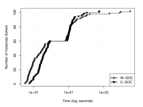
Figure 3: Runtime Profiles for the Two SOC Relaxations.

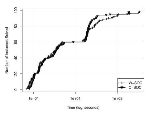
Figure 4: Runtime Profiles for the Two QC Relaxations.

Comparison of SOC formulations

Section V proposed two equivalent formulations of the second-order cone constraints for power flow relaxations. Although both formulations define the same convex set, it is unclear if they have the same performance characteristics. For example, the current-based constraint (C-SOC) has more constraints and more variables than the voltage-product constraint (W-SOC). All other aspects being equal, one would expect (C-SOC) to be slower than (W-SOC). This section investigates the performance implications of these two formulations on both the QC and SOC power flow relaxations. Four power flow relaxations are considered, W-SOC (Model 4), C-SOC (Model 4 with (C-SOC)), W-QC (Model 5 with (W-SOC)), and C-QC (Model 5). To test the performance of these relaxations, each model is evaluated on 105 state-of-the-art AC-OPF transmission system test cases from the NESTA v0.4.0 archive [35]. Figure 3 compares the two variants of the SOC relaxation and Figure 4 compares two variants on the QC relaxation.

Both figures indicate that the two formulations are very similar for small test cases but, on the larger test cases (i.e., with more than 1000 buses), the C-QC formulation has a faster convergence rate, in IPOPT. This suggests that, despite its increased size, the C-QC formulation originally presented in [4] is preferable from a performance standpoint and that the C-SOC formulation may be preferable on very large networks (e.g. above 9000 buses).

References

- [1] X. Bai, H. Wei, K. Fujisawa, and Y. Wang, “Semidefinite programming for optimal power flow problems,” International Journal of Electrical Power & Energy Systems, vol. 30, no. 6–7, pp. 383 – 392, 2008.
- [2] R. Jabr, “Radial distribution load flow using conic programming,” IEEE Transactions on Power Systems, vol. 21, no. 3, pp. 1458–1459, Aug 2006.
- [3] M. Farivar, C. Clarke, S. Low, and K. Chandy, “Inverter var control for distribution systems with renewables,” in 2011 IEEE International Conference on Smart Grid Communications (SmartGridComm), Oct 2011, pp. 457–462.
- [4] H. Hijazi, C. Coffrin, and P. Van Hentenryck, “Convex quadratic relaxations of mixed-integer nonlinear programs in power systems,” Published online at http://www.optimization-online.org/DB_HTML/2013/09/4057.html, 2013.
- [5] D. Molzahn and I. Hiskens, “Moment-based relaxation of the optimal power flow problem,” in Power Systems Computation Conference (PSCC), 2014, Aug 2014, pp. 1–7.
- [6] ——, “Sparsity-exploiting moment-based relaxations of the optimal power flow problem,” Power Systems, IEEE Transactions on, vol. PP, no. 99, pp. 1–13, 2014.
- [7] J. Lavaei and S. Low, “Zero duality gap in optimal power flow problem,” IEEE Transactions on Power Systems, vol. 27, no. 1, pp. 92 –107, feb. 2012.
- [8] S. Low, “Convex relaxation of optimal power flow - part i: Formulations and equivalence,” IEEE Transactions on Control of Network Systems, vol. 1, no. 1, pp. 15–27, March 2014.
- [9] ——, “Convex relaxation of optimal power flow - part ii: Exactness,” IEEE Transactions on Control of Network Systems, vol. 1, no. 2, pp. 177–189, June 2014.
- [10] P. Kundur, Power System Stability and Control. McGraw-Hill Professional, 1994.
- [11] K. Purchala, L. Meeus, D. Van Dommelen, and R. Belmans, “Usefulness of DC power flow for active power flow analysis,” Power Engineering Society General Meeting, pp. 454–459, 2005.
- [12] R. Zimmerman, C. Murillo-S andnchez, and R. Thomas, “Matpower: Steady-state operations, planning, and analysis tools for power systems research and education,” IEEE Transactions on Power Systems, vol. 26, no. 1, pp. 12 –19, feb. 2011.
- [13] C. Carleton and P. Van Hentenryck, “A linear-programming approximation of ac power flows,” Forthcoming in INFORMS Journal on Computing, 2014.
- [14] R. Madani, S. Sojoudi, and J. Lavaei, “Convex relaxation for optimal power flow problem: Mesh networks,” in Signals, Systems and Computers, 2013 Asilomar Conference on, Nov 2013, pp. 1375–1382.
- [15] J. Taylor and F. Hover, “Convex models of distribution system reconfiguration,” IEEE Transactions on Power Systems, vol. 27, no. 3, pp. 1407–1413, Aug 2012.
- [16] A. Gomez Esposito and E. Ramos, “Reliable load flow technique for radial distribution networks,” IEEE Transactions on Power Systems, vol. 14, no. 3, pp. 1063–1069, Aug 1999.
- [17] R. Jabr, “Optimal power flow using an extended conic quadratic formulation,” IEEE Transactions on Power Systems, vol. 23, no. 3, pp. 1000–1008, Aug 2008.
- [18] S. Sojoudi and J. Lavaei, “Physics of power networks makes hard optimization problems easy to solve,” in Power and Energy Society General Meeting, 2012 IEEE, July 2012, pp. 1–8.
- [19] F. Capitanescu, J. M. Ramos, P. Panciatici, D. Kirschen, A. M. Marcolini, L. Platbrood, and L. Wehenkel, “State-of-the-art, challenges, and future trends in security constrained optimal power flow,” Electric Power Systems Research, vol. 81, no. 8, pp. 1731 – 1741, 2011. [Online]. Available: http://www.sciencedirect.com/science/article/pii/S0378779611000885
- [20] B. Stott and O. Alsac, “Optimal power flow — basic requirements for real-life problems and their solutions,” self published, available from brianstott@ieee.org, Jul 2012.
- [21] J. Momoh, R. Adapa, and M. El-Hawary, “A review of selected optimal power flow literature to 1993. i. nonlinear and quadratic programming approaches,” IEEE Transactions on Power Systems, vol. 14, no. 1, pp. 96 –104, feb 1999.
- [22] J. Momoh, M. El-Hawary, and R. Adapa, “A review of selected optimal power flow literature to 1993. ii. newton, linear programming and interior point methods,” IEEE Transactions on Power Systems, vol. 14, no. 1, pp. 105 –111, feb 1999.
- [23] A. Verma, “Power grid security analysis: An optimization approach,” Ph.D. dissertation, Columbia University, 2009.
- [24] K. Lehmann, A. Grastien, and P. Van Hentenryck, “AC-Feasibility on Tree Networks is NP-Hard,” IEEE Transactions on Power Systems, 2015 (to appear).
- [25] B. Subhonmesh, S. Low, and K. Chandy, “Equivalence of branch flow and bus injection models,” in Communication, Control, and Computing (Allerton), 2012 50th Annual Allerton Conference on, Oct 2012, pp. 1893–1899.
- [26] L. Vandenberghe and S. Boyd, “Semidefinite programming,” SIAM Review, vol. 38, no. 1, pp. 49–95, 1996. [Online]. Available: http://dx.doi.org/10.1137/1038003
- [27] R. M. Freund, “Introduction to Semidefinite Programming (SDP),” Published online at http://ocw.mit.edu/courses/electrical-engineering-and-computer-science/6-251j-introduction-to-mathematical-programming-fall-2009/readings/MIT6_251JF09_SDP.pdf, Sept. 2009, accessed: 23/02/2015.
- [28] F. Capitanescu, I. Bilibin, and E. Romero Ramos, “A comprehensive centralized approach for voltage constraints management in active distribution grid,” Power Systems, IEEE Transactions on, vol. 29, no. 2, pp. 933–942, March 2014.
- [29] E. Romero-Ramos, J. Riquelme-Santos, and J. Reyes, “A simpler and exact mathematical model for the computation of the minimal power losses tree,” Electric Power Systems Research, vol. 80, no. 5, pp. 562 – 571, 2010. [Online]. Available: http://www.sciencedirect.com/science/article/pii/S0378779609002570
- [30] G. McCormick, “Computability of global solutions to factorable nonconvex programs: Part i convex underestimating problems,” Mathematical Programming, vol. 10, pp. 146–175, 1976.
- [31] B. Lesieutre, D. Molzahn, A. Borden, and C. DeMarco, “Examining the limits of the application of semidefinite programming to power flow problems,” in 49th Annual Allerton Conference on Communication, Control, and Computing (Allerton), 2011, sept. 2011, pp. 1492 –1499.
- [32] A. Wächter and L. T. Biegler, “On the implementation of a primal-dual interior point filter line search algorithm for large-scale nonlinear programming,” Mathematical Programming, vol. 106, no. 1, pp. 25–57, 2006.
- [33] W. Bukhsh, A. Grothey, K. McKinnon, and P. Trodden, “Local solutions of the optimal power flow problem,” IEEE Transactions on Power Systems, vol. 28, no. 4, pp. 4780–4788, Nov 2013.
- [34] S. Bose, S. Low, T. Teeraratkul, and B. Hassibi, “Equivalent relaxations of optimal power flow,” IEEE Transactions on Automatic Control, vol. PP, no. 99, pp. 1–1, 2014.
- [35] C. Coffrin, D. Gordon, and P. Scott, “NESTA, The Nicta Energy System Test Case Archive,” CoRR, vol. abs/1411.0359, 2014. [Online]. Available: http://arxiv.org/abs/1411.0359
- [36] R. C. U.K., “The hsl mathematical software library,” Published online at http://www.hsl.rl.ac.uk/, accessed: 30/10/2014.
- [37] A. Castillo and R. P. O Neill, “Computational performance of solution techniques applied to the acopf,” Published online at http://www.ferc.gov/industries/electric/indus-act/market-planning/opf-papers/acopf-5-computational-testing.pdf, January 2013, accessed: 17/12/2014.
- [38] R. Fourer, D. M. Gay, and B. Kernighan, “AMPL: A Mathematical Programming Language,” in Algorithms and Model Formulations in Mathematical Programming, S. W. Wallace, Ed. New York, NY, USA: Springer-Verlag New York, Inc., 1989, pp. 150–151.
- [39] J. Lavaei, “Opf solver,” Published online at http://www.ee.columbia.edu/~lavaei/Software.html, oct. 2014, accessed: 22/02/2015.
- [40] R. Madani, M. Ashraphijuo, and J. Lavaei, “Promises of conic relaxation for contingency-constrained optimal power flow problem,” Published online at http://www.ee.columbia.edu/~lavaei/SCOPF_2014.pdf, 2014, accessed: 22/02/2015.
- [41] K. C. Toh, M. Todd, and R. H. T t nc , “Sdpt3 – a matlab software package for semidefinite programming,” Optimization Methods and Software, vol. 11, pp. 545–581, 1999.
- [42] D. Bienstock, M. Chertkov, and S. Harnett, “Chance-constrained optimal power flow: Risk-aware network control under uncertainty,” SIAM Review, vol. 56, no. 3, pp. 461–495, 2014. [Online]. Available: http://dx.doi.org/10.1137/130910312
- [43] C. Coffrin, H. Hijazi, and P. Van Hentenryck, “Network Flow and Copper Plate Relaxations for AC Transmission Systems,” CoRR, vol. abs/1506.05202, 2015. [Online]. Available: http://arxiv.org/abs/1506.05202
- [44] C. Coffrin, H. Hijazi, K. Lehmann, and P. Van Hentenryck, “Primal and dual bounds for optimal transmission switching,” Proceedings of the 18th Power Systems Computation Conference (PSCC’14), Wroclaw, Poland, 2014.
- [45] R. Jabr, “Optimization of ac transmission system planning,” IEEE Transactions on Power Systems, vol. 28, no. 3, pp. 2779–2787, Aug 2013.
- [46] H. Hijazi and S. Thiebaux, “Optimal ac distribution systems reconfiguration,” Proceedings of the 18th Power Systems Computation Conference (PSCC’14), Wroclaw, Poland, 2014.
- [47] J. Taylor and F. Hover, “Conic ac transmission system planning,” IEEE Transactions on Power Systems, vol. 28, no. 2, pp. 952–959, May 2013.