High Dimensional and Banded Vector Autoregressions

Abstract

We consider a class of vector autoregressive models with banded coefficient matrices. The setting represents a type of sparse structure for high-dimensional time series, though the implied autocovariance matrices are not banded. The structure is also practically meaningful when the order of component time series is arranged appropriately. The convergence rates for the estimated banded autoregressive coefficient matrices are established. We also propose a Bayesian information criterion for determining the width of the bands in the coefficient matrices, which is proved to be consistent. By exploring some approximate banded structure for the auto-covariance functions of banded vector autoregressive processes, consistent estimators for the auto-covariance matrices are constructed.

Abstract

This supplementary material is organized as follows. We provide the detailed proofs of Theorems 1-4, respectively, in Sections A.1-A.4. Section A.5 presents Proposition 1 and its proof, showing the consistency of generalized Bayesian Information criterion stated in Remark 1 in the paper. In Section A.6, we present the consistency of the marginal Bayesian information criterion selector $\widehat{k}$ in a more general setting when $k_{0}\to\infty$. Some technical lemmas and their proofs are collected in Section A.7. Section A.8 presents some additional simulation results.

Keywords: Banded auto-coefficient matrices; BIC; Frobenius norm; Vector autoregressive model.

1 Introduction

The demand for modelling and forecasting high-dimensional time series arises from panel studies of economic, social and natural phenomena, financial market analysis, communication engineering and other domains. When the dimension of time series is even moderately large, statistical modelling is challenging, as vector autoregressive and moving average models suffer from lack of identification, over-parameterization and flat likelihood functions. While pure vector autoregressive models are perfectly identifiable, their usefulness is often hampered by the lack of proper means of reducing the number of parameters.

In many practical situations it is enough to collect the information from neighbour variables, though the definition of neighbourhoods is case-dependent. For example, sales, prices, weather indices or electricity consumptions influenced by temperature depend on those at nearby locations, in the sense that the information from farther locations may become redundant given that from neighbours. See, for example, Can and Mebolugbe (1997) for a house price example which exhibits such a dependence structure. In this paper, we propose a class of vector autoregressive models to cater for such dynamic structures. We assume that the autoregressive coefficient matrices are banded, i.e., non-zero coefficients form a narrow band along the main diagonal. The setting specifies explicit autoregression over neighbour component series only. Nevertheless, non-zero cross correlations among all component series may still exist, as the implied auto-covariance matrices are not banded. This is an effective way to impose sparse structure, as the number of parameters in each autoregressive coefficient matrix is reduced from $p^{2}$ to $O(p)$, where $p$ denotes the number of time series. In practice, a banded structure may be employed by arranging the order of component series appropriately. The ordering can be deduced from subject knowledge aided by statistical tools such as Bayesian information criterion; see Section 5.2. With the imposed banded structure, we propose least squares estimators for the autoregressive coefficient matrices which attain the convergence rate $(p/n)^{1/2}$ under the Frobenius norm and $(\log p/n)^{1/2}$ under the spectral norm when $p$ diverges together with the length $n$ of time series.

In practice the maximum width of the non-zero coefficient bands in the coefficient matrices, which is called the bandwidth, is unknown. We propose a marginal Bayesian information criterion to identify the true bandwidth. It is shown that this criterion leads to consistent bandwidth determination when both $n$ and $p$ tend to infinity.

We also address the estimation of the autocovariance functions for high-dimensional banded autoregressive models. Although the autocovariance matrices of a banded process are unlikely to be banded, they admit some asymptotic banded approximations when the covariance of innovations is banded. Because of this property, the band-truncated sample autocovariance matrices are consistent estimators with the convergence rate $\log(n/\log p)(\log p/n)^{1/2}$, which is faster than that for the standard banding covariance estimators Bickel and Levina (2008). See also Wu and Pourahmadi (2009), Bickel and Gel (2011) and Leng and Li (2011) for the estimation of the banded covariance matrices of time series.

Most existing work on high-dimensional autoregressive models draws inspiration from recent developments in high-dimensional regression. For example, Hsu et al. (2008) proposed lasso penalization for subset autoregression. Haufe et al. (2010) introduced the group sparsity for coefficient matrices and advocated use of group lasso penalization. A truncated weighted lasso and group lasso penalization approaches were proposed by Shojaie and Michailidis (2010) and Basu et al. (2015), respectively, to explore graphical Granger causality. Basu and Michailidis (2015) focused on stable Gaussian processes and investigated the theoretical properties of $L_{1}$-regularized estimates of transition matrix in sparse autoregressive models. Bolstad et al. (2011) inferred sparse causal networks through vector autoregressive processes and proposed a group lasso procedure. Kock and Callot (2015) established oracle inequalities for high-dimensional vector autoregressive models. Han and Liu (2015) proposed an alternative Dantzig-type penalization and formulated the estimation problem into a linear program. Chen et al. (2013) studied sparse covariance and precision matrix in high dimensional time series under a general dependence structure.

2 Methodology

2.1 Banded vector autoregressive models

Let $\textit{y}_{t}$ be a $p\times 1$ time series defined by

$$\textit{y}_{t}={A}_{1}\textit{y}_{t-1}+\cdots+{A}_{d}\textit{y}_{t-d}+\varepsilon_{t},$$ (1)

where $\varepsilon_{t}$ is the innovation at time $t$, $E(\varepsilon_{t})=0$ and $\text{var}(\varepsilon_{t})=E(\varepsilon_{t}\varepsilon_{t}^{{\mathrm{\scriptscriptstyle T}}})={\Sigma}_{\varepsilon}$, and $\varepsilon_{t}$ is independent of $\textit{y}_{t-1},\textit{y}_{t-2},\ldots$. Furthermore, all the coefficient matrices ${A}_{1},\ldots,{A}_{d}$ are banded in the sense that

$$a_{ij}^{(\ell)}=0,\quad|i-j|>k_{0},~{}\ell=1,\ldots,d,$$ (2)

where $a_{ij}^{(\ell)}$ denotes the $(i,j)$-th element of ${A}_{\ell}$. Thus the maximum number of non-zero elements in each row of ${A}_{\ell}$ is the bandwidth $2k_{0}+1$, and $k_{0}$ is called the bandwidth parameter. We assume that $k_{0}\geq 0$ and $d\geq 1$ are fixed integers, and $p\gg k_{0},d$. Our goal is to determine $k_{0}$ and to estimate the banded coefficient matrices ${A}_{1},\ldots,{A}_{d}$. For simplicity, we assume that the autoregressive order $d$ is known, as the order-determination problem has already been thoroughly studied; see, e.g., Chapter 4 of Lütkepohl (2007).

Under the condition $\det({I}_{p}-{A}_{1}z-\cdots-{A}_{d}z^{d})\neq 0$ for any $|z|\leq 1$, model (1) admits a weakly stationary solution $\{\textit{y}_{t}\}$, where ${I}_{p}$ denotes the $p\times p$ identity matrix. Throughout this paper, $\textit{y}_{t}$ refers to this stationary process. If, in addition, $\varepsilon_{t}$ is independent and identically distributed, $\textit{y}_{t}$ is also strictly stationary.

In model (1), we do not require $\text{var}(\varepsilon_{t})={\Sigma}_{\varepsilon}$ to be banded, but even if it is, the autocovariance matrices are not necessarily banded; see (12) below. Therefore, the proposed banded model is applicable when the linear dynamics of each component series depend predominately on its neighbour series, though there may be non-zero correlations among all component series of $\textit{y}_{t}$.

2.2 Estimating banded autoregressive coefficient matrices

Since each row of ${A}_{\ell}$ has at most $2k_{0}+1$ non-zero elements, there are at most $(2k_{0}+1)d$ regressors in each row on the right-hand side of (1). For $i=1,\ldots,p$, let ${\beta}_{i}$ be the column vector obtained by stacking the non-zero elements in the $i$-th rows of ${A}_{1},\ldots,{A}_{d}$ together. Let $\tau_{i}$ denote the length of ${\beta}_{i}$. Then

$$\tau_{i}\equiv\tau_{i}(k_{0})=\Big{\{}\begin{array}[]{ll}(2k_{0}+1)d,&i=k_{0}+1,\,k_{0}+2,\ldots,p-k_{0},\\ (2k_{0}+1-j)d,&i=k_{0}+1-j\;\;{\rm or}\;\;p-k_{0}+j,\quad j=1,\ldots,k_{0}.\end{array}$$ (3)

Now (1) can be written as

$$y_{i,t}=\textit{x}_{i,t}^{{\mathrm{\scriptscriptstyle T}}}{\beta}_{i}+\varepsilon_{i,t},\qquad i=1,\ldots,p,$$ (4)

where $y_{i,t}$, $\varepsilon_{i,t}$ are respectively the $i$-th component of $\textit{y}_{t}$ and $\varepsilon_{t}$ and $\textit{x}_{i,t}$ is the $\tau_{i}\times 1$ vector consisting of the corresponding components of $\textit{y}_{t-1},\ldots,\textit{y}_{t-d}$. Consequently, the least squares estimator of ${\beta}_{i}$ based on (4) is

$$\widehat{{\beta}}_{i}=({X}_{i}^{{\mathrm{\scriptscriptstyle T}}}{X}_{i})^{-1}{X}_{i}^{{\mathrm{\scriptscriptstyle T}}}\textit{y}_{(i)},$$ (5)

where $\textit{y}_{(i)}=(y_{i,d+1},\ldots,y_{i,n})^{{\mathrm{\scriptscriptstyle T}}}$, and ${X}_{i}$ is an $(n-d)\times\tau_{i}$ matrix with $\textit{x}_{i,d+j}^{{\mathrm{\scriptscriptstyle T}}}$ as its $j$-th row.

By estimating ${\beta}_{i}$, $i=1,\ldots,p$, separately based on (5), we obtain the least squares estimators $\widehat{A}_{1},\ldots,\widehat{A}_{d}$ for the coefficient matrices in (1). Furthermore, the resulting residual sum of squares is

$$\textsc{RSS}_{i}\equiv\textsc{RSS}_{i}(k_{0})=\textit{y}_{(i)}^{{\mathrm{\scriptscriptstyle T}}}\{{I}_{n-d}-{X}_{i}({X}_{i}^{{\mathrm{\scriptscriptstyle T}}}{X}_{i})^{-1}{X}_{i}^{{\mathrm{\scriptscriptstyle T}}}\}\textit{y}_{(i)}.$$ (6)

We write this as a function of $k_{0}$ to stress that the above estimation presupposes that the bandwidth is $(2k_{0}+1)$ in the sense of (2).

2.3 Determination of bandwidth

In practice the bandwidth is unknown and we need to estimate $k_{0}$. We propose to determine $k_{0}$ based on the marginal Bayesian information criterion,

$$\textsc{BIC}_{i}(k)=\log\textsc{RSS}_{i}(k)+\frac{1}{n}d\tau_{i}(k)C_{n}\log(p\vee n),\qquad i=1,\ldots,p,$$ (7)

where $\textsc{RSS}_{i}(k)$ and $\tau_{i}(k)$ are defined, respectively, in (6) and (3), $p\vee n=\max(p,n)$, and $C_{n}>0$ is some constant which diverges together with $n$; see Condition 2. We often take $C_{n}$ to be $\log\log n$. An estimator for $k_{0}$ is

$$\widehat{k}=\max_{1\leq i\leq p}\big{\{}\arg\min_{1\leq k\leq K}\textsc{BIC}_{i}(k)\big{\}},$$ (8)

where $K\geq 1$ is a prescribed integer. Our numerical study shows that the procedure is insensitive to the choice of $K$ provided $K\geq k_{0}$. In practice, we often take $K$ to be $[n^{1/2}]$ or choose $K$ by checking the curvature of $\textsc{BIC}_{i}(k)$ directly.

Remark 1. If the order $d$ is unknown, we can modify the criterion in (8) as follows. Let $\textsc{RSS}_{i}(k,\ell)$ and $\tau_{i}(k,\ell)$ be defined similarly to (6) and (3). The marginal Bayesian information criterion is

$$\widetilde{\textsc{BIC}}_{i}(k,\ell)=\log\textsc{RSS}_{i}(k,\ell)+\frac{1}{n}\tau_{i}(k,\ell)C_{n}\log(p\vee n),\qquad i=1,\ldots,p.$$ (9)

Let $L$ be a prescribed integer upper bound on $d$ and often taken to be $10$ or $[n^{1/2}]$. Let

$$(\widehat{k}_{i},\widehat{d}_{i})=\arg\min_{1\leq k\leq K,1\leq\ell\leq L}\widetilde{\textsc{BIC}}_{i}(k,\ell),~{}i=1,\ldots,p,$$

and $\widehat{k}=\max_{1\leq i\leq p}\widehat{k}_{i}$ and $\widehat{d}=\max_{1\leq i\leq p}\widehat{d}_{i}.$ Proposition 1 in the Supplementary Material shows that under Conditions 1–4 in Section 3.1, $\mbox{pr}(\widehat{k}=k_{0},\widehat{d}=d)\to 1$ as $n$ and $p\to\infty$.

Remark 2. The banded structure of the coefficient matrices $A_{1},\ldots,A_{d}$ depends on the order of the component series of $\textit{y}_{t}$. In principle it is possible to derive a complete data-driven method to deduce the optimal ordering which minimizes the bandwidth, but such a procedure is computationally burdensome for large $p$. For most applications meaningful orderings are suggested by practical consideration. We can then calculate

$$\textsc{BIC}=\sum_{i=1}^{p}\textsc{BIC}_{i}(\widehat{k})$$ (10)

for each suggested ordering, and choose the ordering which minimizes (10). In expression (10), $\textsc{BIC}_{i}(\cdot)$ and $\widehat{k}$ are defined as in (7) and (8). Two real data examples in Section 5.2 indicate that this scheme works well in applications.

3 Asymptotic properties

3.1 Regularity conditions

For vector $\textit{v}=(v_{1},\ldots,v_{j})$ and matrix ${B}=(b_{ij})$, let

$$\|\textit{v}\|_{q}=\Big{(}\sum_{j=1}^{p}|v_{j}|^{q}\Big{)}^{1/q},\quad\|\textit{v}\|_{\infty}=\max_{1\leq j\leq p}|v_{j}|,\quad\|{B}\|_{q}=\max_{\|\textit{v}\|_{q}=1}\|{B}\textit{v}\|_{q},\quad\|{B}\|_{F}=\Big{(}\sum_{i,j}b_{ij}^{2}\Big{)}^{1/2},$$

i.e., $\|\cdot\|_{q}$ denotes the $\ell_{q}$ norm of a vector or matrix, and $\|\cdot\|_{F}$ denotes the Frobenius norm of a matrix.

First we note that the model (1) can be formulated as,

$$\widetilde{\textit{y}}_{t}=\widetilde{{A}}\widetilde{\textit{y}}_{t-1}+\widetilde{\varepsilon}_{t},$$

where

$$\widetilde{\textit{y}}_{t}=\left(\begin{array}[]{cccc}\textit{y}_{t}\\ \textit{y}_{t-1}\\ \vdots\\ \textit{y}_{t-d+1}\end{array}\right),\quad\widetilde{{A}}=\left(\begin{array}[]{cccc}{A}_{1}&{A}_{2}&\cdots&{A}_{d}\\ {I}_{p}&\textit{0}_{p}&\cdots&\cdots\\ \vdots&\cdots&\vdots&\cdots\\ \textit{0}&\cdots&{I}_{p}&\textit{0}\\ \end{array}\right),\quad\widetilde{\varepsilon}_{t}=\left(\begin{array}[]{cccc}\varepsilon_{t}\\ \textit{0}_{p\times 1}\\ \vdots\\ \textit{0}_{p\times 1}\end{array}\right).$$ (11)

Now we list the regularity conditions required for our asymptotic results.

Condition 1. For $\widetilde{A}$ defined in (11), $\|\widetilde{{A}}\|_{2}\leq C$ and $\|\widetilde{{A}}^{j_{0}}\|_{2}\leq\delta^{j_{0}}$, where $C>0$, $\delta\in(0,1)$ and ${j_{0}}\geq 1$ are constants free of $n$ and $p$, and ${j_{0}}$ is an integer.

Condition 1’. For $\widetilde{A}$ defined in (11), $\|\widetilde{{A}}^{j_{0}}\|_{2}\leq\delta^{j_{0}}$, $\|\widetilde{{A}}\|_{\infty}\leq C$ and $\|\widetilde{{A}}^{j_{0}}\|_{\infty}\leq\delta^{j_{0}}$, where $C>0$, $\delta\in(0,1)$ and ${j_{0}}\geq 1$ are constants free of $n$ and $p$, and ${j_{0}}$ is an integer.

Condition 2. Let $a_{ij}^{(\ell)}$ be the $(i,j)$-th element of ${A}_{\ell}$. For each $i=1,\ldots,p$, $|a^{(\ell)}_{i,i+k_{0}}|$ or $|a^{(\ell)}_{i,i-k_{0}}|$ is greater than $\{C_{n}k_{0}n^{-1}\log(p\vee n)\}^{1/2}$ for some $1\leq\ell\leq d$, where $C_{n}\to\infty$ as $n\to\infty$.

Condition 3. The minimal eigenvalue $\lambda_{\min}\{\text{cov}(\textit{y}_{t})\}\geq\kappa_{1}$ and $\max_{1\leq i\leq p}|\sigma_{ii}|\leq\kappa_{2}$ for some positive constants $\kappa_{1}$ and $\kappa_{2}$ free of $p$, where $\sigma_{ii}$ is the $i$-th diagonal element of $\text{cov}(\textit{y}_{t})$, and $\lambda_{\min}(\cdot)$ denotes the minimum eigenvalue.

Condition 4. The innovation process $\{\varepsilon_{t},\,t=0,\pm 1,\pm 2,\ldots\}$ is independent and identically distributed with zero mean and covariance ${\Sigma}_{\varepsilon}$. Furthermore, one of the two assertions holds:

(i)   $\max_{1\leq i\leq p}E(|\varepsilon_{i,t}|^{2q})\leq C$ and $p=O(n^{\beta})$, where $q>2$, $\beta\in(0,(q-2)/4)$ and $C>0$ are some constants free of $n$ and $p$;

(ii)    $\max_{1\leq i\leq p}E\{\exp(\lambda_{0}|\varepsilon_{i,t}|^{2\alpha})\}\leq C$ and $\log p=o\{n^{{\alpha}/(2-\alpha)}\}$, where $\lambda_{0}>0$, $\alpha\in(0,1]$ and $C>0$ are constants free of $n$ and $p$.

Provided $\{\varepsilon_{t}\}$ is independent and identically distributed, Condition 1 implies that $\textit{y}_{t}$ is strictly stationary and that for any $j\geq 1$, $\|\widetilde{{A}}^{j}\|_{2}\leq C\delta^{j}$ with some constant $C>0$ and $\delta\in(0,1)$. The independent and identically distributed assumption in Condition 4 is imposed to simplify the proofs but is not essential. Condition 2 ensures that the bandwidth $(2k_{0}+1)$ is asymptotically identifiable, as $\left\{n^{-1}\log(p\vee n)\right\}^{1/2}$ is the minimum order of a non-zero coefficient to be identifiable; see, e.g., Luo and Chen (2013). Condition 3 guarantees that the covariance matrix $\text{var}(y_{t})$ is strictly positive definite. Condition 4 specifies the two asymptotic modes: (i) high-dimensional cases with $p=O(n^{\beta})$, and (ii) ultra high-dimensional cases with $\log p=o\{n^{{\alpha}/{(2-\alpha)}}\}$.

3.2 Asymptotic theorems

We first state the consistency of the selector $\widehat{k}$, defined in (8), for determining the bandwidth parameter $k_{0}$.

Theorem 1.

Under Conditions 1–4, $\mbox{pr}(\widehat{k}=k_{0})\to 1$ as $n\to\infty$.

Remark 3. In Theorem 1, $k_{0}$ is assumed to be fixed, as in applications small $k_{0}$ is of particular interest. But we can allow the bandwidth parameter $k_{0}$ to diverge as $n,p\to\infty$. To show its consistency, the regularity conditions would need to be strengthened. To be specific, if $k_{0}\ll C_{n}^{-1}n/\log(p\vee n)$, $\mbox{pr}(\widehat{k}=k_{0})\to 1$ as $n\to\infty$ under Conditions 1’ and 2–4 in Section 3.1; see the Supplementary Material.

Since $k_{0}$ is unknown, we replace it by $\widehat{k}$ in the estimation procedure for ${A}_{1},\ldots,{A}_{d}$ described in Section 2.2, and still denote the resulted estimators by $\widehat{A}_{1},\ldots,\widehat{A}_{d}$. Theorem 2 addresses their convergence rates.

Theorem 2.

Let Conditions 1–4 hold. As $n\to\infty$, it holds for $j=1,\ldots,d$ that

$$\big{\|}\widehat{{A}}_{j}-{A}_{j}\big{\|}_{F}=O_{P}\Big{\{}(p/n)^{1/2}\Big{\}},~{}~{}\big{\|}\widehat{{A}}_{j}-{A}_{j}\big{\|}_{2}=O_{P}\Big{\{}(\log p/n)^{1/2}\Big{\}}.$$

Conditions 4(i) and 4(ii) impose, respectively, a high moment condition and an exponential tail condition on the innovation distribution. Although the convergence rates in Theorem 2 have the same expressions in terms of $n$ and $p$, due to the different conditions imposed on them in Conditions 4(i) and 4(ii), the actual convergence rates are different under the two settings. For example, Condition 4(i) allows $p$ to grow in the order $n^{\beta}$, which implies the convergence rate ${(\log n/n)}^{1/2}$ for $\widehat{{A}}_{j}$ under the spectral norm. On the other hand, Condition 4(ii) may allow $p$ to diverge at the rate $\exp\{n^{\alpha/(2-\alpha)-2\epsilon}\}$ for a small constant $\epsilon>0$, and the implied convergence rate for $\widehat{{A}}_{j}$ under the spectral norm is $n^{1/2+\epsilon-\alpha/(4-2\alpha)}$.

4 Estimation for auto-covariance functions

For the banded vector autoregressive process $\textit{y}_{t}$ defined by (1), the auto-covariance function ${\Sigma}_{j}=\text{cov}(\textit{y}_{t},\textit{y}_{t+j})$ is unlikely to be banded. For example for a stationary banded autoregressive process with order 1, it can be shown that

$${\Sigma}_{0}\equiv\text{var}(\textit{y}_{t})={\Sigma}_{\varepsilon}+\sum_{i=1}^{\infty}{A}_{1}^{i}{\Sigma}_{\varepsilon}({A}_{1}^{{\mathrm{\scriptscriptstyle T}}})^{i}.$$ (12)

For any banded matrices ${B}_{1}$ and ${B}_{2}$ with bandwidths $2k_{1}+1$ and $2k_{2}+1$, respectively, the product ${B}_{1}{B}_{2}$ is a banded matrix with the enlarged bandwidth $2(k_{1}+k_{2})+1$ in general. Thus ${\Sigma}_{0}$ presented in (12) is not a banded matrix. Nevertheless if $\text{var}(\varepsilon_{t})={\Sigma}_{\varepsilon}$ is also banded, Theorem 3 shows that ${\Sigma}_{j}$ can be approximated by some banded matrices.

Condition 5. The matrix ${\Sigma}_{\varepsilon}$ is banded with bandwidth $2s_{0}+1$ and $\|{\Sigma}_{\varepsilon}\|_{1}\leq C<\infty$, where $C,s_{0}>0$ are constants independent of $p$, and $s_{0}$ is an integer.

Theorem 3.

Let Conditions 1 and 5 hold. For any integers $r,j\geq 0$, there exists a banded matrix ${\Sigma}_{j}^{(r)}$ with bandwidth $2\{(2r+j)k_{0}+s_{0}\}+1$ such that

$$\|{\Sigma}_{j}^{(r)}-{\Sigma}_{j}\|_{2}\leq C_{1}\,\delta^{2(r+j)+1},~{}~{}\|{\Sigma}_{j}^{(r)}-{\Sigma}_{j}\|_{1}\leq C_{2}\,r\,\delta^{2(r+j)+1},$$

where $C_{1}$ and $C_{2}$ are positive constants independent of $r$ and $p$, and $\delta\in(0,1)$ is specified in Condition 1.

Under Condition 5, ${\Sigma}_{0}^{(r)}={\Sigma}_{\varepsilon}+\sum_{1\leq i\leq r}{A}_{1}^{i}{\Sigma}_{\varepsilon}({A}_{1}^{{\mathrm{\scriptscriptstyle T}}})^{i}$ is a banded matrix with bandwidth $2(2rk_{0}+s_{0})+1$. Theorem 3 ensures that the norms of the difference ${\Sigma}_{0}-{\Sigma}_{0}^{(r)}=\sum_{i>r}{A}_{1}^{i}{\Sigma}_{\varepsilon}({A}_{1}^{{\mathrm{\scriptscriptstyle T}}})^{i}$ admit the required upper bounds. Theorem 3 also paves the way for estimating ${\Sigma}_{j}$ using the banding method of Bickel and Levina (2008), as ${\Sigma}_{j}$ can be approximated by a banded matrix with a bounded error and thus may be effectively treated as a banded matrix. To this end, we define the banding operator as follows: for any matrix ${H}=(h_{ij})$, $B_{r}({H})=\big{\{}h_{ij}I(|i-j|\leq r)\big{\}}$. Then the banding estimator for ${\Sigma}_{j}$ is defined as

$$\widehat{{\Sigma}}_{j}^{(r_{n})}=B_{r_{n}}(\widehat{{\Sigma}}_{j}),~{}~{}\widehat{{\Sigma}}_{j}=\frac{1}{n}\sum_{t=1}^{n-j}(\textit{y}_{t}-\bar{\textit{y}})(\textit{y}_{t+j}-\bar{\textit{y}})^{{\mathrm{\scriptscriptstyle T}}},~{}~{}\bar{\textit{y}}=\frac{1}{n}\sum_{t=1}^{n}\textit{y}_{t},$$ (13)

where $r_{n}=C\log(n/\log p),$ and $C>0$ is a constant greater than $\left(-4\log\delta\right)^{-1}$. Theorem 4 presents the convergence rates for $\widehat{{\Sigma}}_{j}^{(r_{n})}$, which are faster than those in Bickel and Levina (2008), due to the approximate banded structure in Theorem 3.

Theorem 4.

Assume that Conditions 1–5 hold. Then for any integer $j\geq 0$, as $n,p\to\infty$,

$$\|\widehat{{\Sigma}}_{j}^{(r_{n})}-{\Sigma}_{j}\|_{2}=O_{P}\Big{\{}r_{n}{\left({n^{-1}\log p}\right)}^{1/2}+\delta^{2(r_{n}+j)+1}\Big{\}}=O_{P}\Big{\{}\log(n/\log p){\left({n^{-1}\log p}\right)}^{1/2}\Big{\}},$$

and

$$\|\widehat{{\Sigma}}_{j}^{(r_{n})}-{\Sigma}_{j}\|_{1}=O_{P}\Big{\{}\log(n/\log p)\left(n^{-1}\log p\right)^{1/2}\Big{\}}.$$

In practice we need to specify $r_{n}$. An ideal selection would be $r_{n}=\arg\min_{r}R_{j}(r)$, where

$$R_{j}(r)=E(\|\widehat{{\Sigma}}_{j}^{(r)}-{\Sigma}_{j}\|_{1}),$$

but in practice this is unavailable because ${\Sigma}_{j}$ is unknown. We replace it by an estimator obtained via a wild bootstrap. To this end, let $u_{1},\ldots,u_{n}$ be independent and identically distributed with $E(u_{t})=\text{var}(u_{t})=1$. A bootstrap estimator for ${\Sigma}_{j}$ is defined as

$${\Sigma}_{j}^{*}={1\over n}\sum_{t=1}^{n-j}u_{t}(\textit{y}_{t}-\bar{\textit{y}})(\textit{y}_{t+j}-\bar{\textit{y}})^{{\mathrm{\scriptscriptstyle T}}}.$$

For example, we may draw $u_{t}$ from the standard exponential distribution. Consequently the bootstrap estimator for $R_{j}(r)$ is defined as

$$R_{j}^{*}(r)=E\big{\{}\|B_{r}({\Sigma}_{j}^{*})-\widehat{{\Sigma}}_{j}\|_{1}\big{|}\,\textit{y}_{1},\ldots,\textit{y}_{n}\big{\}}.$$

We choose $r_{n}$ to minimize $R_{j}^{*}(r)$. In practice we use the approximation

$$R_{j}^{*}(r)\approx\frac{1}{q}\sum_{k=1}^{q}\|B_{r}({\Sigma}_{j,k}^{*})-\widehat{{\Sigma}}_{j}\|_{1},$$ (14)

where ${\Sigma}_{j,1}^{*},\ldots,{\Sigma}_{j,q}^{*}$ are $q$ bootstrap estimates for ${\Sigma}_{j}$, obtained by repeating the above wild bootstrap scheme $q$ times, and $q$ is a large integer.

5 Numerical properties

5.1 Simulations

In this section, we evaluate the finite-sample properties of the proposed methods for the model

$$\textit{y}_{t}={A}\textit{y}_{t-1}+\varepsilon_{t},$$

where $\{\varepsilon_{t}\}$ are independent and $N(0,I_{p})$. We consider two settings for the banded coefficient matrix ${A}=(a_{ij})$ as follows:

(i) $\{a_{ij};\;|i-j|\leq k_{0}\}$ are generated independently from $U[-1,1]$. Since the spectral norm of ${A}$ must be smaller than 1, we re-scale ${A}$ by $\eta{A}/\|{A}\|_{2}$, where $\eta$ is generated from $U[0.3,1.0)$;

(ii) $\{a_{ij};\;|i-j|<k_{0}\}$ are generated independently from the mixture distribution $\xi\cdot 0+(1-\xi)\cdot N(0,1)$ with $\mbox{pr}(\xi=1)=0.4$. The elements $\{a_{ij};|i-j|=k_{0}\}$ are drawn independently from $-4$ and $4$ with probability 0.5 each. Then ${A}$ is rescaled as in (i) above.

In (ii), there are about $0.4(2k_{0}-1)p$ zero elements within the band, i.e., ${A}$ is sparser than in (i).

We set $n=200$, $p=100,200,400,800$, and $k_{0}=1,2,3,4$. We repeat each setting 500 times. We only report the results with $K=15$ in (8), as the results with other values of $K\geq k_{0}$ are similar. Table 1 lists the relative frequencies of the occurrence of the events $\{\widehat{k}=k\},\;\{\widehat{k}>k_{0}\}$ and $\{\widehat{k}<k_{0}\}$ over the 500 replications. Overall $\widehat{k}$ under-estimates $k_{0}$, especially when $k_{0}=3$ or 4. In fact when $k_{0}=4$, $\widehat{k}$ chose 3 most times. The constraint $\|{A}\|<1$ makes most non-zero elements small or very small when $p$ is large, and that only the coefficients at least as large as $\surd{\log(p\vee n)/n}$ are identifiable; see Condition 2. Estimation performs better in setting (ii) than in setting (i), as Condition 2 is more likely to hold at the boundaries of the band in setting (ii).

The Bayesian information criterion (7) is defined for each row separately. One natural alternative would be

$$\textsc{BIC}(k)=\sum_{i=1}^{p}\log\textsc{RSS}_{i}(k)+{1\over n}|\widetilde{\tau}(k)|C_{n}\log(p\vee n),$$

where $\widetilde{\tau}(k)=(2p+1)k-k^{2}-k$ is the total number of parameters in the model. This leads to the following estimator for the bandwidth parameter,

$$\widetilde{k}=\arg\min_{1\leq k\leq K}\textsc{BIC}(k).$$ (15)

Although this joint approach can be shown to be consistent, its finite sample performance, reported in Table 2, is worse than that of the marginal Bayesian information criterion (7), presented in Table 1.

We also calculate both $L_{1}$ and $L_{2}$ errors in estimating the banded coefficient matrix ${A}$. The means and the standard deviations of the errors for setting (i) are reported in Table 3. Table 3 also reports results from estimating ${A}$ using the true values for the bandwidth parameter $k_{0}$. The accuracy loss in estimating ${A}$ caused by unknown $k_{0}$ is almost negligible. The results for setting (ii) are similar and are therefore omitted.

To evaluate the estimation performance for the auto-covariance matrices ${\Sigma}_{0}$ and ${\Sigma}_{1}$, we set $k_{0}=3$, and the spectral norm of ${A}$ at 0.8. Furthermore, we let $\varepsilon_{t}$ be independent and $N(0,{\Sigma}_{\varepsilon})$ now, where ${\Sigma}_{\varepsilon}={B}{B}^{{\mathrm{\scriptscriptstyle T}}}$ and ${B}=(b_{ij}),b_{11}=1,b_{ij}=0.8I(|i-j|=1)+0.6I(i=j)$, $i>1$ or $j>1$. Table 4 lists the average estimation errors and the standard deviations over 100 replications, measured by matrix $L_{1}$-norm. We also report Monte Carlo results for a thresholded estimator and the sample covariance estimator. For the banded estimator, we choose $r$ to minimize the bootstrap loss defined in (14) with $q=100$. For the thresholded estimator, the thresholding parameter is selected in the same manner. Table 4 shows that the proposed banding method performs much better than the thresholded estimator since it adapts directly to the underlying structure, while the sample covariance performs much worse than both the banding and threshold methods.

5.2 Real data examples

Consider first the weekly temperature data across 71 cities in China from 1 January 1990 to 17 December 17 2000, i.e., $p=71$ and $n=572$. Fig.1 displays the weekly temperature of Ha’erbin, Shanghai and Hangzhou, showing strong seasonal behavior with period 52 weeks. Therefore, we set the seasonal period to be 52 and estimate the seasonal effects by taking averages of the same weeks across different years. The deseasonalized series, i.e., the original series subtracting estimated seasonal effects, are denoted by $\{\,\textit{y}_{t};\;t=1,\ldots,572\,\}$, and each $\textit{y}_{t}$ has 71 components.

Naturally we would order the 71 cities according to their geographic locations. However the choice is not unique. For example, we may order the cities from north to south, from west to east, from northwest to southeast, or from southwest to northeast. By setting $d=1$, each ordering leads to a different banded autoregressive model with order 1. We compare those four models by one-step ahead, and two-step ahead post-sample prediction for the last 30 data points in the series. To select an optimum model, we compute (10) for these four orderings. These numerical results and the selected bandwidth parameters $\widehat{k}$ are reported in Table 5. Three out of those four models select $\widehat{k}=2$, while the model based on the ordering from west to east picks $\widehat{k}=4$. Overall the model based on the ordering from southwest to northeast is preferred, which also has the minimum one-step ahead post-sample predictive errors. The performances of the four models in terms of the prediction are very close.

Also included in Table 5 are the post-sample predictive errors of the sparse autoregressive model with order 1 obtained via lasso by minimizing

$$\sum_{t=2}^{n}\|\textit{y}_{t}-{A}\textit{y}_{t-1}\|^{2}+\sum_{i,j=1}^{p}\lambda_{i}|a_{ij}|,$$

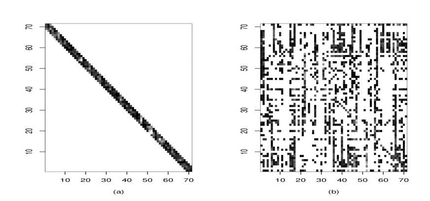
Figure 2: Example 1: (a) Estimated banded coefficient matrix $\widehat{A}$ for the model based on the ordering from southwest to northeast, and (b) estimated sparse coefficient matrix $\widetilde{A}$ by lasso. White points represent zeros entries and gray or black points represent nonzero entries. The larger the absolute value of a coeffcient is, the darker the colour is.

where $\lambda_{1},\ldots,\lambda_{p}$ are tuning parameters estimated by five-fold cross-validation as in Bickel and Levina (2008). The prediction accuracy of the sparse model via lasso is comparable to those of the banded autoregressive models, though slightly worse, especially for the two-step ahead prediction. However the lack of any structure in the estimated sparse coefficient matrix $\widetilde{{A}}$, displayed in Fig.2(b), makes such fits difficult to interpret. In contrast, the banded coefficient matrix, depicted in Fig.2(a), is attractive.

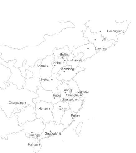
Figure 3: Location plot of 21 provinces and province-level municipalities in China, where Shanghai is a province-level municipality, and Ha’erbin, Hangzhou and Nanjing are the capitals of Heilongjiang, Zhejiang, and Jiangsu provinces, respectively.

As a second example, we consider the daily sales of a clothing brand in 21 provinces in China from 1 January 2008 to 9 December 2012, i.e., $n=1812,\;p=21$. Fig.3 plots the relative geographical positions of 21 provinces and province-level municipalities. We first subtract each of the 21 series by its mean. Similar to the example above, we order the 21 provinces according to the four different geographic orientations, and fit a banded autoregressive model with order 1 for each ordering. The selected bandwidth parameters, the values according to (10) and the post sample prediction errors for the last 30 data points in the series are reported in Table 6. We also rank the series according to their geographic distances to Heilongjiang, the most northwestern province; see Fig.3. This results in a different ordering to that from north to south. Table 6 indicates that the minimum bandwidth parameter $\widehat{k}$ is 3, attained by the ordering based on the distances to Heilongjiang, followed by $\widehat{k}=4$ attained by the north-to-south ordering. The post-sample prediction performances of those two models are almost the same, and are better than those of the other three banded models and the sparse autoregressive model.

The ordering based on the direction from northwest to southeast leads to $\widehat{k}=12$. Therefore the corresponding banded model has 21 regressors for some components according to (3), i.e., no banded structure is observed in this case. Fig.3 indicates that the ordering from northwest to southeast puts together some provinces which are distance away from each other. Hence this is certainly a wrong ordering as far as the banded autoregressive structure is concerned.

The estimated coefficient matrix $\widehat{A}$ for the banded vector autoregressive model with order 1 based on the distances to Heilongjiang and the estimated $\widetilde{A}$ by lasso for the autoregressive model with order 1 are plotted in Fig.4. The banded model facilitates an easy interpretation, i.e., the sales in the neighbour provinces are closely associated with each other. The lasso fitting cannot reveal this phenomenon.

Supplementary Material

Supplementary material available at Biometrika online includes proofs of Theorems 1-4, the consistency of generalized Bayesian information criterion defined by (9) in Section 2.3 and the consistency of the marginal Bayesian information criterion in the setting $k_{0}\to\infty$, as well as the detailed proofs of all the lemmas in this paper.

Table 1: Relative frequencies (%) for the occurrence of the events $\{\widehat{k}=k\},\;\{\widehat{k}>k_{0}\}$ and $\{\widehat{k}<k_{0}\}$ in a simulation study with $500$ replications, where $\widehat{k}$ is defined in (8).

			Setting (i)			Setting (ii)
		$\{\widehat{k}=k_{0}\}$	$\{\widehat{k}>k_{0}\}$	$\{\widehat{k}<k_{0}\}$	$\{\widehat{k}=k_{0}\}$	$\{\widehat{k}>k_{0}\}$	$\{\widehat{k}<k_{0}\}$
	$k_{0}=1$	82	17	1	98	2	0
$p=100$	$k_{0}=2$	87	8	5	95	3	2
	$k_{0}=3$	73	6	21	83	2	15
	$k_{0}=4$	55	14	31	64	2	34
	$k_{0}=1$	91	9	0	97	3	0
$p=200$	$k_{0}=2$	89	4	7	93	2	5
	$k_{0}=3$	65	3	32	83	0	17
	$k_{0}=4$	54	1	45	63	2	35
	$k_{0}=1$	95	5	0	99	1	0
$p=400$	$k_{0}=2$	87	2	11	90	1	9
	$k_{0}=3$	66	2	32	76	1	23
	$k_{0}=4$	45	1	54	60	0	40
	$k_{0}=1$	97	3	0	100	0	0
$p=800$	$k_{0}=2$	86	1	13	91	1	8
	$k_{0}=3$	59	1	40	67	1	32
	$k_{0}=4$	40	0	60	52	0	48

Table 2: Relative frequencies (%) for the occurrence of the events $\{\widetilde{k}=k\},\;\{\widetilde{k}>k_{0}\}$ and $\{\widetilde{k}<k_{0}\}$ in a simulation study with $500$ replications, where $\widetilde{k}$ is defined in (15).

			Setting (i)			Setting (ii)
		$\{\widetilde{k}=k_{0}\}$	$\{\widetilde{k}>k_{0}\}$	$\{\widetilde{k}<k_{0}\}$	$\{\widetilde{k}=k_{0}\}$	$\{\widetilde{k}>k_{0}\}$	$\{\widetilde{k}<k_{0}\}$
	$k_{0}=1$	64	0	36	88	0	12
$p=100$	$k_{0}=2$	42	0	58	63	0	37
	$k_{0}=1$	56	0	44	84	0	16
$p=200$	$k_{0}=2$	32	0	68	55	0	45
	$k_{0}=1$	48	0	52	83	0	17
$p=400$	$k_{0}=2$	23	0	77	45	0	55
	$k_{0}=1$	44	0	56	76	0	24
$p=800$	$k_{0}=2$	11	0	89	41	0	59

Table 3: Means ($\times 10^{2}$) with their corresponding standard deviations ($\times 10^{2}$) in parentheses of the errors in estimating ${A}$ under setting ($i$) in a simulation study with $n=200$ and $500$ replications.

		With estimated $k_{0}$		With true $k_{0}$
$p$		$\|\widehat{{A}}-{A}\|_{1}$	$\|\widehat{{A}}-{A}\|_{2}$	$\|\widehat{{A}}-{A}\|_{1}$	$\|\widehat{{A}}-{A}\|_{2}$
	$k_{0}=1$	38 (6)	27 (3)	37 (5)	27 (3)
$p=100$	$k_{0}=2$	54 (6)	33 (3)	53 (5)	33 (3)
	$k_{0}=3$	70 (8)	39 (4)	69 (7)	38 (3)
	$k_{0}=4$	85 (10)	43 (5)	85 (8)	43 (3)
	$k_{0}=1$	40 (6)	28 (3)	40 (5)	28 (3)
$p=200$	$k_{0}=2$	58 (7)	35 (3)	58 (6)	35 (3)
	$k_{0}=3$	74 (8)	40 (4)	74 (6)	40 (3)
	$k_{0}=4$	90 (11)	46 (5)	88 (7)	45 (3)
	$k_{0}=1$	43 (5)	30 (3)	42 (4)	30 (3)
$p=400$	$k_{0}=2$	60 (6)	36 (3)	60 (5)	36 (3)
	$k_{0}=3$	77 (8)	42 (4)	76 (6)	42 (3)
	$k_{0}=4$	95 (14)	48 (7)	93 (7)	46 (3)
	$k_{0}=1$	44 (4)	31 (2)	44 (4)	31 (2)
$p=800$	$k_{0}=2$	63 (5)	37 (3)	62 (5)	37 (2)
	$k_{0}=3$	81 (9)	43 (5)	80 (6)	43 (2)
	$k_{0}=4$	98 (14)	49 (7)	96 (7)	47 (2)

Table 4: Means with their corresponding standard deviations in parentheses of the errors in estimating autocovariance matrices in a simulation study with $n=200$ and $100$ replications.

		$\|\widehat{{\Sigma}}_{n,0}-{\Sigma}_{0}\|_{1}$			$\|\widehat{{\Sigma}}_{n,1}-{\Sigma}_{1}\|_{1}$
	Banding	Thresholding	Sample	Banding	Thresholding	Sample
		Matrix $L_{1}$-Norm			Matrix $L_{1}$-Norm
$p=100$	2.1 (0.04)	2.6 (0.02)	14 (0.07)	2.9 (0.03)	3.5 (0.04)	14 (0.07)
$p=200$	2.7 (0.04)	3.4 (0.03)	29 (0.02)	3.1 (0.03)	4.2 (0.04)	30 (0.02)
$p=400$	2.3 (0.02)	2.9 (0.02)	55 (0.02)	2.8 (0.03)	3.7 (0.02)	55 (0.02)
$p=800$	2.7 (0.03)	3.4 (0.02)	112 (0.03)	2.9 (0.03)	3.9 (0.03)	110 (0.04)
		Spectral Norm			Spectral Norm
$p=100$	1.1 (0.01)	1.4 (0.02)	4.0 (0.07)	1.4 (0.01)	1.7 (0.02)	3.7 (0.02)
$p=200$	1.3 (0.03)	1.7 (0.02)	6.5 (0.03)	1.5 (0.01)	1.9 (0.01)	6.1 (0.02)
$p=400$	1.2 (0.01)	1.6 (0.01)	10 (0.03)	1.3 (0.01)	1.9 (0.01)	9.2 (0.02)
$p=800$	1.4 (0.02)	1.8 (0.01)	17 (0.03)	1.4 (0.01)	2.3 (0.02)	15 (0.03)

Table 5: Results of Example 1: Estimated bandwidth parameters, Bayeysian information criterion values and average one-step-ahead and two-step-ahead post-sample predictive errors over 71 cities with their corresponding standard errors in parentheses.

Ordering	$\widehat{k}$	BIC	One-step ahead	Two-step ahead
north to south	2	552.5	1.543 (1.170)	1.622 (1.245)
west to east	4	555.9	1.545 (1.152)	1.602 (1.247)
northwest to southeast	2	552.4	1.552 (1.167)	1.624 (1.249)
southwest to northeast	2	551.9	1.538 (1.160)	1.617 (1.253)
Lasso	-	-	1.545 (1.172)	1.632 (1.250)

Table 6: Results of Example 2: Estimated bandwidth parameters, Bayeysian information criterion values and average one-step-ahead and two-step-ahead post-sample predictive errors over 21 provinces with their corresponding standard errors in parentheses.

Ordering	$\widehat{k}$	BIC	One-step ahead	Two-step ahead
north to south	4	114.9	0.314 (0.377)	0.407 (0.386)
west to east	7	115.2	0.323 (0.363)	0.409 (0.386)
northwest to southeast	12	115.2	0.322 (0.361)	0.409 (0.395)
southwest to northeast	5	115.1	0.316 (0.374)	0.407 (0.385)
distance to Heilongjiang	3	114.7	0.313 (0.378)	0.407 (0.386)
Lasso	-	-	0.322 (0.362)	0.410 (0.393)

Figure 1: Deseasonalized weekly temperature in degrees Celsius $(^{\circ}\mbox{C})$ from January 1990 to December 2000, where Ha’erbin, Shanghai and Nanjing correspond to the plots from top to bottom.

Figure 4: Example 2: (a) Estimated banded coefficient matrix $\widehat{A}$ for the model based on the ordering using distances to Heilongjiang, and (b) estimated sparse coefficient matrix $\widetilde{A}$ by lasso. White points represent zeros entries and gray or black points represent nonzero entries. The larger the absolute value of a coeffcient is, the darker the colour is.

A.1 Proof of Theorem 1

Without loss of generality, we consider the VAR(1) model with $\|{A}\|_{1}\leq\delta<1$. Our goal is to prove that $\mbox{pr}(\widehat{k}=k_{0})\to 1$, i.e., $\mbox{pr}(\widehat{k}\neq k_{0})\to 0$. If $\widehat{k}\neq k_{0}$, then either $\widehat{k}>k_{0}$ or $\widehat{k}<k_{0}$ holds. Hence it suffices to show that $\mbox{pr}(\widehat{k}<k_{0})\to 0$ and $\mbox{pr}(\widehat{k}>k_{0})\to 0$. Our proof follows the arguments in Wang, et al. (2009).

Consider the first case. Observe that $\mbox{pr}(\widehat{k}<k_{0})\leq\mbox{pr}(\widehat{k}_{i}<k_{0})$ for some $i\in\{1,\ldots,p\}$ and the event $(\widehat{k}_{i}<k_{0})$ imply $\{\min_{k<k_{0}}\textsc{BIC}_{i}(k)<\textsc{BIC}_{i}(k_{0})\}.$ To prove $\mbox{pr}(\widehat{k}<k_{0})\to 0$, we only need to show that

$$\mbox{pr}\{\min_{k<k_{0}}\textsc{BIC}_{i}(k)<\textsc{BIC}_{i}(k_{0})\}\to 0$$

for some $i$. Suppose that we have shown that there exists a constant $\eta>0$ and an event $\mathcal{A}_{n}$ such that $\mbox{pr}(\mathcal{A}_{n})\to 1$ as $n\to\infty$ and on the event $\mathcal{A}_{n}$,

$$\textsc{RSS}_{i}(k)-\textsc{RSS}_{i}(k_{0})\geq\eta\textsc{RSS}_{i}(k_{0})(a_{i,i-k_{0}}^{2}+a_{i,i+k_{0}}^{2}),$$ (A.1)

for sufficiently large $n$, where $a_{j,k}$ is the $(j,k)$-element of ${A}_{1}$. On the event $\mathcal{A}_{n}$ with large $n$, $\log\textsc{RSS}_{i}(k)-\log\textsc{RSS}_{i}(k_{0})\geq\log\{1+\eta(a_{i,i-k_{0}}^{2}+a_{i,i+k_{0}}^{2})\}.$ Note that $\log(1+x)\geq\min(0.5x,\log 2)$ for any $x>0$. Consequently, with probability tending to one, $\log\textsc{RSS}_{i}(k)-\log\textsc{RSS}_{i}(k_{0})$ can be further bounded below by $\min\{0.5\eta(a_{i,i-k_{0}}^{2}+a_{i,i+k_{0}}^{2}),\log 2\}.$ Condition 3 implies that for some $i^{*}\in\{1,\ldots,p\}$, $a_{i^{*},i^{*}-k_{0}}^{2}+a_{i^{*},i^{*}+k_{0}}^{2}\gg C_{n}\log p/n$ as $n\to\infty$. Hence, it follows that, with probability tending to 1,

$$\min_{k<k_{0}}\textsc{BIC}_{i^{*}}(k)-\textsc{BIC}_{i^{*}}(k_{0}) > \min\{0.5\eta(a_{i^{*},i^{*}-k_{0}}^{2}+a_{i^{*},i^{*}+k_{0}}^{2}),\log 2\}$$

$$-C_{n}k_{0}n^{-1}\log(p\vee n)>0,$$

where $p\vee n=\max(p,n)$. Hence, $\mbox{pr}\{\min_{k<k_{0}}\textsc{BIC}_{i^{*}}(k)<\textsc{BIC}_{i^{*}}(k_{0})\}\to 0$ and thus $\mbox{pr}(\widehat{k}<k_{0})\to 0$.

Let us prove (A.1). For $k<k_{0}$, denote ${H}_{i,k}={X}_{i,k}\big{(}{X}_{i,k}^{{\mathrm{\scriptscriptstyle T}}}{X}_{i,k}\big{)}^{-1}{X}_{i,k}^{{\mathrm{\scriptscriptstyle T}}}$, ${X}_{i,k_{0}}=({S}_{i,k}^{(1)},{X}_{i,k},{S}_{i,k}^{(2)})$ and ${\beta}_{i,k_{0}}=(\textit{b}_{i,1}^{{\mathrm{\scriptscriptstyle T}}},{\beta}_{i,k}^{{\mathrm{\scriptscriptstyle T}}},\textit{b}_{i,2}^{{\mathrm{\scriptscriptstyle T}}})^{{\mathrm{\scriptscriptstyle T}}}$, where ${X}_{i,k}$ is defined similar to (4) in Section 2.2 except that $k_{0}$ is replaced by $k$. Then $\textsc{RSS}_{i}(k)=\textit{y}_{(i)}^{{\mathrm{\scriptscriptstyle T}}}\big{(}{I}_{n-1}-{H}_{i,k}\big{)}\textit{y}_{(i)},$ and by Lemma 5 (ii) or Lemma 6 (ii), we have

$$\textsc{RSS}_{i}(k)-\textsc{RSS}_{i}(k_{0})=(\textit{b}_{i,1}^{{\mathrm{\scriptscriptstyle T}}},\textit{b}_{i,2}^{{\mathrm{\scriptscriptstyle T}}})({S}_{i,k}^{(1)},{S}_{i,k}^{(2)})^{{\mathrm{\scriptscriptstyle T}}}({I}_{n-1}-{H}_{i,k})({S}_{i,k}^{(1)},{S}_{i,k}^{(2)})\left(\begin{array}[]{cc}\textit{b}_{i,1}\\ \textit{b}_{i,2}\end{array}\right)+o_{P}(1).$$

From Lemma 5 (i) or Lemma 6 (i) and Lemma 7, there exists a small constant $\eta>0$ such that, with probability tending to one,

$$\lambda_{\min}\big{\{}({S}_{i,k}^{(1)},{S}_{i,k}^{(2)})^{{\mathrm{\scriptscriptstyle T}}}({I}-{H}_{i,k})({S}_{i,k}^{(1)},{S}_{i,k}^{(2)})\big{\}}>\eta(1+\eta)n\sigma_{i}^{2},$$

and $\textsc{RSS}_{i}(k_{0})\leq n\sigma_{i}^{2}(1+\eta)$. Therefore, (A.1) follows.

Now we turn to the overfitting case, i.e., $\mbox{pr}(\widehat{k}>k_{0})\to 0$. For $k>k_{0}$, set

$${X}_{i,k}=({S}_{i,k}^{(1)},{X}_{i,k_{0}},{S}_{i,k}^{(2)}),{\beta}_{i,k}=(\textit{0}^{{\mathrm{\scriptscriptstyle T}}},{\beta}_{i,k_{0}}^{{\mathrm{\scriptscriptstyle T}}},\textit{0}^{{\mathrm{\scriptscriptstyle T}}})^{{\mathrm{\scriptscriptstyle T}}},{S}_{i,k}=({S}_{i,k}^{(1)},{S}_{i,k}^{(2)}),$$

and $\widetilde{{S}}_{i,k}=\big{(}{I}_{n-1}-{H}_{i,k_{0}}\big{)}{S}_{i,k}$. Let $\eta$ be an arbitrary but fixed positive constant and define

$$\mathcal{B}_{n}=\Big{\{}\inf_{k_{0}\leq k\leq K}{\inf_{1\leq i\leq p}}\frac{\textsc{RSS}_{i}(k)}{n\sigma_{i}^{2}}>(1-\eta)\Big{\}},$$

$$\mathcal{C}_{n}=\underset{k_{0}\leq k\leq K}{\bigcup_{1\leq i\leq p}}\Big{\{}\lambda_{\min}^{-1}(n^{-1}\widetilde{{S}}_{i,k}^{{\mathrm{\scriptscriptstyle T}}}\widetilde{{S}}_{i,k})<\kappa_{1}^{-1}(1+\eta),\sup_{1\leq j\leq k-k_{0}}\left|\left(n^{-1}{S}_{i,k}^{T}{S}_{i,k}\right)_{jj}\right|<\kappa_{2}(1+\eta)\Big{\}}.$$

We first give an upper bound on $\textsc{RSS}_{i}(k_{0})-\textsc{RSS}_{i}(k)$ for $k>k_{0}$. For each $i$, $\textsc{RSS}_{i}(k)$ can be rewritten as

$$\textsc{RSS}_{i}(k)=\inf_{\textit{b}}\|\textit{y}_{(i)}-{X}_{i,k}\textit{b}\|^{2}=\inf_{\textit{b}_{1},\textit{b}_{2}}\|\textit{y}_{(i)}-{X}_{i,k_{0}}\textit{b}_{1}-{S}_{i}\textit{b}_{2}\|^{2}.$$

It can be verified that $\textsc{RSS}_{i}(k_{0})=\|({I}_{n-1}-{H}_{i,k_{0}})\textit{y}_{(i)}\|^{2}$ and

$$\textsc{RSS}_{i}(k)=\textsc{RSS}_{i}(k_{0})-\|\widetilde{{S}}_{i}^{(k)}\widehat{\textit{b}}_{2}\|^{2},$$

where $\widehat{\textit{b}}_{2}=\left(\widetilde{{S}}_{i,k}^{T}\widetilde{{S}}_{i,k}\right)^{-1}\widetilde{{S}}_{i,k}^{T}{e}_{(i)}$. Then on the event $\mathcal{C}_{n}$ we have

$$\textsc{RSS}_{i}(k_{0})-\textsc{RSS}_{i}(k) = {e}_{(i)}^{{\mathrm{\scriptscriptstyle T}}}\widetilde{{S}}_{i,k}(\widetilde{{S}}_{i,k}^{{\mathrm{\scriptscriptstyle T}}}\widetilde{{S}}_{i,k})^{-1}\widetilde{{S}}_{i,k}^{{\mathrm{\scriptscriptstyle T}}}{e}_{(i)}$$

$$\leq \kappa_{1}^{-1}(1+\eta)|\tau_{i}(k)-\tau_{i}(k_{0})|\sup_{j,k\leq p}\big{|}n^{-1/2}{e}_{(j)}^{{\mathrm{\scriptscriptstyle T}}}({I}_{n-1}-{H}_{i,k_{0}})\textit{x}_{(k)}\big{|}^{2}.$$

Define

$$\mathcal{D}_{n}=\Big{\{}\sup_{j,k\leq p}\big{|}n^{-1/2}{e}_{(j)}^{{\mathrm{\scriptscriptstyle T}}}({I}_{n-1}-{H}_{i,k_{0}})\textit{x}_{(k)}\big{|}^{2}\sigma_{i}^{-2}<\frac{\kappa_{1}(1-\eta)}{1+\eta}C_{n}\log(p\vee n)\Big{\}}.$$

On the set $\mathcal{B}_{n}\cap\mathcal{C}_{n}\cap\mathcal{D}_{n}$, for all $k$ with $k_{0}\leq k\leq K$,

$$\textsc{RSS}_{i}(k_{0})-\textsc{RSS}_{i}(k) < \sigma_{i}^{2}(1-\eta)|\tau_{i}(k)-\tau_{i}(k_{0})|C_{n}\log(p\vee n)$$

$$< \textsc{RSS}_{i}(k)C_{n}|\tau_{i}(k)-\tau_{i}(k_{0})|n^{-1}\log(p\vee n).$$

Note that $\log(1+x)\leq x$ for any $x>0$. Hence, for all $k$ with $k_{0}<k\leq K$, on the set $\mathcal{B}_{n}\cap\mathcal{C}_{n}\cap\mathcal{D}_{n}$,

$$\textsc{BIC}_{i}(k)-\textsc{BIC}_{i}(k_{0}) = \log\textsc{RSS}_{i}(k)-\log\textsc{RSS}_{i}(k_{0})+C_{n}|\tau_{i}(k)-\tau_{i}(k_{0})|n^{-1}\log(p\vee n)$$

$$\geq -\left\{\textsc{RSS}_{i}(k_{0})-\textsc{RSS}_{i}(k)\right\}\left\{\textsc{RSS}_{i}(k)\right\}^{-1}$$

$$+C_{n}|\tau_{i}(k)-\tau_{i}(k_{0})|n^{-1}\log(p\vee n)>0,$$

which indicates that over the set $\mathcal{B}_{n}\cap\mathcal{C}_{n}\cap\mathcal{D}_{n}$, we have that $\widehat{k}\leq k_{0}$. To prove that $\mbox{pr}(\widehat{k}>k_{0})\to 0$, it suffices to show that $\mbox{pr}\left\{\big{(}\mathcal{B}_{n}\cap\mathcal{C}_{n}\cap\mathcal{D}_{n}\big{)}^{c}\right\}\to 0$. In fact, it follows from Lemma 7 and Lemma 5 or 6 (i) that $\mbox{pr}\left(\mathcal{B}_{n}^{c}\right)\to 0$ and $\mbox{pr}\left(\mathcal{C}_{n}^{c}\right)\to 0$. It remains to show that $\mbox{pr}\left(\mathcal{D}_{n}^{c}\right)\to 0$. Let ${\Sigma}_{i,k}=n^{-1}E\left({X}_{i,k}^{{\mathrm{\scriptscriptstyle T}}}{X}_{i,k}\right)$, $\widehat{{\Sigma}}_{i,k}=n^{-1}{X}_{i,k}^{{\mathrm{\scriptscriptstyle T}}}{X}_{i,k}$, where $E(X)$ denotes the expectation of $X$. Set $\widetilde{{H}}_{i,k}=n^{-1}{X}_{i,k}{\Sigma}_{i,k}^{-1}{X}_{i,k}^{{\mathrm{\scriptscriptstyle T}}}$, and $\widetilde{\textit{x}}_{(k)}=({I}_{n-1}-\widetilde{{H}}_{i,k})\textit{x}_{(k)}$. On the event $\mathcal{C}_{n}$, we obtain that

$$\sup_{j,k\leq p}\big{|}{e}_{(j)}^{{\mathrm{\scriptscriptstyle T}}}({I}_{n-1}-{H}_{i,k_{0}})\textit{x}_{(k)}\big{|}$$

$$\leq\sup_{j,k\leq p}\big{|}{e}_{(j)}^{{\mathrm{\scriptscriptstyle T}}}\widetilde{\textit{x}}_{(k)}\big{|}+\sup_{j,k\leq p}\big{|}{e}_{(j)}^{{\mathrm{\scriptscriptstyle T}}}({H}_{i,k_{0}}-\widetilde{{H}}_{i,k_{0}})\textit{x}_{(k)}\big{|}$$

$$\leq\sup_{j,k\leq p}\big{|}{e}_{(j)}^{{\mathrm{\scriptscriptstyle T}}}\widetilde{\textit{x}}_{(k)}\big{|}+n^{-1}\sup_{j,k\leq p}\|{e}_{(j)}^{{\mathrm{\scriptscriptstyle T}}}{X}_{i,k_{0}}\|_{2}\|{\Sigma}_{i,k_{0}}^{-1}\|_{2}\|\widehat{{\Sigma}}_{i,k_{0}}^{-1}\|_{2}\|\widehat{{\Sigma}}_{i,k_{0}}-{\Sigma}_{i,k_{0}}\|_{2}\|{X}_{i,k_{0}}^{{\mathrm{\scriptscriptstyle T}}}\textit{x}_{(k)}\|_{2}$$

$$\leq\sup_{j,k\leq p}\big{|}{e}_{(j)}^{{\mathrm{\scriptscriptstyle T}}}\widetilde{\textit{x}}_{(k)}\big{|}+k_{0}\kappa_{1}^{-2}k_{2}(1+\eta)^{2}\sup_{j,k\leq p}\big{|}{e}_{(j)}^{{\mathrm{\scriptscriptstyle T}}}\textit{x}_{(k)}\big{|}\cdot\|\widehat{{\Sigma}}_{i,k_{0}}-{\Sigma}_{i,k_{0}}\|_{2},$$

where $\sup_{1\leq k\leq p}(n^{-1}\textit{x}_{(k)}\textit{x}_{(k)}^{T})\leq\kappa_{2}(1+\eta)$ is used in the above inequality. Hence, it follows from Lemmas 5 and 6, together with Condition 3, that $\mbox{pr}\left(\mathcal{D}_{n}^{c}\right)\to 0$ as $n\to\infty$. This completes the proof.

A.2 Proof of Theorem 2

Since the autoregressive model with order $d$ can be formulated as a autoregressive model with order 1, without loss of generality, we consider the case of order 1 only. With probability tending to one, $\widehat{k}=k_{0}$, and thus it suffices to consider the set $\mathcal{A}_{n}=\{\widehat{k}=k_{0}\}.$ Over the set $\mathcal{A}_{n}$, for each $i$,

$$\widehat{{\beta}}_{i}-{\beta}_{i}=\left({X}_{i}^{{\mathrm{\scriptscriptstyle T}}}{X}_{i}\right)^{-1}{X}_{i}^{{\mathrm{\scriptscriptstyle T}}}{e}_{(i)}.$$ (A.2)

For each $i$, the law of large numbers for the stationary process case yields that $n^{-1}{X}_{i}^{{\mathrm{\scriptscriptstyle T}}}{X}_{i}$ converges to a positive matrix almost surely, and furthermore, with probability tending to one, $\lambda_{\min}\left(n^{-1}{X}_{i}^{{\mathrm{\scriptscriptstyle T}}}{X}_{i}\right)$ is bounded away from zero. As a matter of fact, if we define

$$\mathcal{B}_{n}=\bigcap_{{1\leq i\leq p}}\left\{\lambda_{\min}\left(n^{-1}{X}_{i}^{{\mathrm{\scriptscriptstyle T}}}{X}_{i}\right)>\kappa_{1}(1-\eta)\right\}$$

with a small constant $\eta\in(0,1)$, then it follows from by Lemma 5 or Lemma 6 under different moment conditions that $P\{\mathcal{B}_{n}\}\to 1$ as $n\to\infty$. Hence, over the event $\mathcal{A}_{n}\cap\mathcal{B}_{n}$,

$$\left\|\widehat{{\beta}}_{i}-{\beta}_{i}\right\|_{2}^{2}\leq\kappa_{1}^{-2}(1-\eta)^{-2}n^{-2}\left\|{e}_{(i)}^{{\mathrm{\scriptscriptstyle T}}}{X}_{i}\right\|^{2}_{2}=C_{1}n^{-2}\left\|{e}_{(i)}^{{\mathrm{\scriptscriptstyle T}}}{X}_{i}\right\|^{2}_{2},$$

where $C_{1}=\kappa_{1}^{-2}(1-\eta)^{-2}>0$. It is not hard to see from Lemma 5(ii) or Lemma 6(ii) that, for all $1\leq i\leq p$, $n^{-1}E\|{X}_{i}^{{\mathrm{\scriptscriptstyle T}}}{e}_{(i)}\|^{2}_{2}\leq C_{2}$ with some constant $C_{2}>0$. Therefore, for a large positive constant $C$, we obtain that

$$\mbox{pr}\left(\left\|\widehat{{A}}_{1}-{A}_{1}\right\|_{F}^{2}>C{n^{-1}p}\right) = \mbox{pr}\left(\left\|\widehat{{A}}_{1}-{A}_{1}\right\|_{F}^{2}>C{n^{-1}p},\mathcal{A}_{n}\cap\mathcal{B}_{n}\right)+\mbox{pr}\left(\mathcal{A}_{n}\cap\mathcal{B}_{n}\right)$$

$$= (Cp)^{-1}n(C_{1}n^{-2})E\left(\sum_{i=1}^{p}\|{X}_{i}^{{\mathrm{\scriptscriptstyle T}}}{e}_{(i)}\|^{2}_{2}\right)+\mbox{pr}\left(\mathcal{A}_{n}\cap\mathcal{B}_{n}\right)$$

$$= {C_{1}C_{2}C^{-1}}+o(1).$$

We establish the convergence rate of $\|\widehat{{A}}_{1}-{A}_{1}\|_{F}$ by taking a sufficiently large $C$.

Now we derive the convergence rate of $\|\widehat{{A}}_{1}-{A}_{1}\|_{2}$. For any matrix ${B}$, $\|{B}\|_{2}^{2}\leq\|{B}\|_{1}\|{B}\|_{\infty}$. Hence, on the event $\mathcal{A}_{n}$,

$$\|\widehat{{A}}_{1}-{A}_{1}\|_{2}\leq\surd{\|\widehat{{A}}_{1}-{A}_{1}\|_{1}}\surd{\|\widehat{{A}}_{1}-{A}_{1}\|_{\infty}}\leq(2k_{0}+1)\sup_{i\leq p,j\leq\tau_{i}}\big{|}\widehat{\beta}_{ij}-\beta_{ij}\big{|},$$

where $\widehat{\beta}_{ij}$ and $\beta_{ij}$ are the $j$-th element of $\widehat{{\beta}}_{i}$ and ${\beta}_{i}$, respectively. Observe from (A.2) that

$$\sup_{i\leq p,j\leq\tau_{i}}\big{|}\widehat{\beta}_{ij}-\beta_{ij}\big{|}=\kappa_{1}^{-1}(1-\eta)^{-1}(2k_{0}+1)\big{(}\sup_{i\leq p,j\leq\tau_{i}}|{e}_{(i)}^{{\mathrm{\scriptscriptstyle T}}}\textit{x}_{(j)}|\big{)},i=1,\ldots,p.$$

Hence, using Lemma 5(ii) or Lemma 6(ii), we have

$$\sup_{i\leq p,j\leq\tau_{i}}\big{|}\widehat{\beta}_{ij}-\beta_{ij}\big{|}=O_{P}\left\{\left(n^{-1}\log p\right)^{1/2}\right\},$$

which shows that

$$\|\widehat{{A}}_{1}-{A}_{1}\|_{2}=O_{P}\left\{\left(n^{-1}\log p\right)^{1/2}\right\}.$$

The proof is completed.

A.3 Proof of Theorem 3

The covariance matrix ${\Sigma}_{0}$ can be expressed as

$${\Sigma}_{0}={\Sigma}_{\varepsilon}+\sum_{j=1}^{\infty}{B}_{j},~{}~{}{B}_{j}={J}\widetilde{{A}}^{j}{J}^{{\mathrm{\scriptscriptstyle T}}}{\Sigma}_{\varepsilon}{J}(\widetilde{{A}}^{{\mathrm{\scriptscriptstyle T}}})^{j}{J}^{{\mathrm{\scriptscriptstyle T}}},~{}~{}j\geq 1,$$

where ${J}=\left({I}_{p\times p},\textit{0}_{p\times(d-1)p}\right)$. Let ${\Phi}_{j}={J}\widetilde{{A}}^{j}{J}^{{\mathrm{\scriptscriptstyle T}}}$, $j\geq 1$. By the companion matrix $\widetilde{{A}}$, we can show that ${\Phi}_{0}={I}_{p}$ and ${\Phi}_{j}=\sum_{k=1}^{\min(j,d)}{\Phi}_{j-k}{A}_{k}$, $j\geq 1$. It is easy to see that for two banded matrices ${F}$ and $G$ with bandwidths $2r_{1}+1$ and $2r_{2}+1$, respectively, the product matrix ${F}G$ is also banded and its bandwidth is at most $2(r_{1}+r_{2})+1$. Therefore, it can be verified that ${\Phi}_{j}$ is banded with bandwidth at most $2jk_{0}+1$ and then ${B}_{j}$ is also banded with its bandwidth at most $2(2jk_{0}+s_{0})+1$ for $j\geq 1$. Take ${\Sigma}_{0}^{(r)}={\Sigma}_{\varepsilon}+\sum_{j=1}^{r}{B}_{j}$, which is banded with the bandwidth at most $2(2rk_{0}+s_{0})+1$, and ${\Sigma}_{0}-{\Sigma}_{0}^{(r)}=\sum_{j=r+1}^{\infty}{B}_{j}$. Note that for any $j\geq 1$, $\|{B}_{j}\|_{2}\leq\|{\Sigma}_{\varepsilon}\|_{2}\|\widetilde{{A}}^{2j}\|_{2}\leq C\delta^{2j}$ for some $C>0$. Write $C_{1}=C\|{\Sigma}_{\varepsilon}\|_{2}\left(1-\delta^{2}\right)^{-1}$. It follows that

$$\|{\Sigma}_{0}-{\Sigma}_{0}^{(r)}\|_{2}\leq\sum_{j=r+1}^{\infty}\|{B}_{j}\|_{2}\leq C\|{\Sigma}_{\varepsilon}\|_{2}\left(1-\delta^{2}\right)^{-1}\delta^{2(r+1)}=C_{1}\delta^{2(r+1)}.$$

By using the inequality $\|{B}_{j}\|_{1}\leq\{2(2jk_{0}+s_{0})+1\}\|{B}_{j}\|_{2}\leq C(2j+1)\delta^{2j}$ for some $C>0$, we obtain

$$\|{\Sigma}_{0}-{\Sigma}_{0}^{(r)}\|_{1}\leq C_{2}r\delta^{2(r+1)}.$$

Other inequalities can be proved analogously. The proof is complete.

A.4 Proof of Theorem 4

Now we prove the convergence rate of $\|\widehat{{\Sigma}}_{n,0}^{(r_{n})}-{\Sigma}_{0}\|_{2}$. First, $\|\widehat{{\Sigma}}_{n,0}^{(r_{n})}-{\Sigma}_{0}\|_{2}$ can be bounded above by

$$\|\widehat{{\Sigma}}_{n,0}^{(r_{n})}-{\Sigma}_{0}^{(r_{n})}\|_{2}+\|{\Sigma}_{0}^{(r_{n})}-{\Sigma}_{0}\|_{2}=R_{n1}+R_{n2}.$$

Similar to Theorem 2, $R_{n1}\leq(4r_{n}k_{0}+2s_{0}+1)\sup_{j,k\leq p}|\widehat{\Sigma}_{jk}-\Sigma_{jk}|$. From Lemma 5(i) or Lemma 6(i), we obtain that

$$R_{n1}=O_{P}\left\{r_{n}\left(n^{-1}\log p\right)^{1/2}\right\}.$$

From Theorem 3, $R_{n2}\leq O(\delta^{2(r_{n}+1)})$. Note that $r_{n}=C\log\{n\log^{-1}(p)\}$ with $C>\left(-4\log\delta\right)^{-1}$. Combining these results, it follows that

$$\|\widehat{{\Sigma}}_{n,0}^{(r_{n})}-{\Sigma}_{0}\|_{2} = O_{P}\Big{\{}r_{n}\left(n^{-1}\log p\right)^{1/2}+\delta^{2(r_{n}+1)}\Big{\}}$$

$$= O_{P}\Big{[}\log\{n\log^{-1}(p)\}\left(n^{-1}\log p\right)^{1/2}\Big{]}.$$

The proofs of other results are similar and omitted.

A.5 Proposition 1 and its proof

PROPOSITION 1. Under Conditions 1-4 in Section 3.1 of the original article, we prove that $\mbox{pr}(\widehat{k}=k_{0},\widehat{d}=d)\to 1$ as $n,p\to\infty$.

Proof of Proposition 1. Our primary goal is to prove that $\mbox{pr}(\widehat{k}=k_{0},\widehat{d}=d)\to 1$, i.e.,

$$\mbox{pr}\{(\widehat{k}\neq k_{0})\cup(\widehat{d}\neq d)\}\to 0.$$

Note that

$$\mbox{pr}\{(\widehat{k}\neq k_{0})\cup(\widehat{d}\neq d)\}\leq\mbox{pr}(\widehat{k}<k_{0})+\mbox{pr}(\widehat{d}<d)+\mbox{pr}(\widehat{k}>k_{0},\widehat{d}>d).$$

We observe that both events $\{\widehat{k}<k_{0}\}$ and $\{\widehat{d}<d\}$ correspond to the underfitting case, where some important variables are missed in the estimated model. Hence, following the proofs of Theorem 1, we can show $\mbox{pr}(\widehat{k}<k_{0})+\mbox{pr}(\widehat{d}<d)\to 0.$

It remains to prove that $\mbox{pr}(\widehat{k}>k_{0},\widehat{d}>d)\to 0$. First look at the event $\mathcal{A}=\big{\{}\widehat{k}>k_{0},\widehat{d}>d\big{\}}$. Define $\mathcal{A}_{1}=\underset{i\leq p}{\cup}\big{\{}\widehat{k}_{i}\geq k_{0},\widehat{d}_{i}>d\big{\}}$, $\mathcal{A}_{2}=\underset{i\leq p}{\cup}\big{\{}\widehat{k}_{i}<k_{0},\widehat{d}_{i}>d\big{\}}$, $\mathcal{A}_{3}=\underset{i\leq p}{\cup}\big{\{}\widehat{k}_{i}>k_{0},\widehat{d}_{i}\geq d\big{\}}$, and $\mathcal{A}_{4}=\underset{i\leq p}{\cup}\big{\{}\widehat{k}_{i}>k_{0},\widehat{d}_{i}<d\big{\}}$. Then $\mathcal{A}\subset\mathcal{A}_{1}\cup\mathcal{A}_{2}\cup\mathcal{A}_{3}\cup\mathcal{A}_{4},$ which implies that it suffices to show $\mbox{pr}(\mathcal{A}_{k})\to 0$ for each $k=1,\ldots,4$. Observe that both events $\mathcal{A}_{1}$ and $\mathcal{A}_{3}$ correspond to the overfitting case, where all important variables as well as some unimportant variables are selected by the estimated model. Hence, following the proofs of Theorem 1, we can show $\mbox{pr}(\mathcal{A}_{1})+\mbox{pr}(\mathcal{A}_{3})\to 0.$

Now we are going to prove $\mbox{pr}(\mathcal{A}_{2})\to 0$ as $n,p\to\infty$. For each $i$, $\{\widehat{k}_{i}<k_{0},\widehat{d}_{i}>d\}$ means $\underset{{k<k_{0},\ell>d}}{\min}\widetilde{\textsc{BIC}}_{i}(k,\ell)<\widetilde{\textsc{BIC}}_{i}(k_{0},d).$ Hence, we only need to show, with probability tending to one,

$$\min_{i\leq p}\min_{k<k_{0},d<\ell\leq L}\left\{\widetilde{\textsc{BIC}}_{i}(k,\ell)-\widetilde{\textsc{BIC}}_{i}(k_{0},d)\right\}>0.$$ (A.3)

Suppose that we have shown that there exists a constant $\eta>0$ and an event $\mathcal{G}_{n}$ such that $\mbox{pr}(\mathcal{G}_{n})\to 1$ as $n\to\infty$ and on the event $\mathcal{G}_{n}$,

$$\min_{i\leq p}\big{\{}\textsc{RSS}_{i}(k,\ell)-\textsc{RSS}_{i}(k_{0},d)-\eta\textsc{RSS}_{i}(k_{0},d)\Delta_{i}\geq 0,$$ (A.4)

for each $k<k_{0}$, $d<\ell<L$ and sufficiently large $n$, where $\Delta_{i}=\sum_{j=1}^{d}\big{\{}(a_{i,i-k_{0}}^{(j)})^{2}+(a_{i,i+k_{0}}^{(j)})^{2}\big{\}}.$ As a result, on the event $\mathcal{G}_{n}$ with large $n$, $\min_{i\leq p}\big{\{}\log\textsc{RSS}_{i}(k,\ell)-\log\textsc{RSS}_{i}(k_{0},d)-\log(1+\eta\Delta_{i})\big{\}}\geq 0.$ Note that $\log(1+x)\geq\min\{0.5x,\log 2\}$ for any $x>0$. Then, with probability tending to one, $\log\textsc{RSS}_{i}(k)-\log\textsc{RSS}_{i}(k_{0})$ can be further bounded below by $\min(0.5\Delta_{i},\log 2).$ Condition 3 implies that $\min_{i\leq p}\Delta_{i}\gg C_{n}n^{-1}\log(p\vee n)$ as $n\to\infty$. Hence, it follows that, with probability tending to 1,

$$\widetilde{\textsc{BIC}}_{i}(k,\ell)-\widetilde{\textsc{BIC}}_{i}(k_{0},d)\geq\min(0.5\eta\Delta_{i},\log 2)-C_{n}\tau_{i}(k_{0},d)n^{-1}\log(p\vee n)>0$$ (A.5)

uniformly for all $k<k_{0},d<\ell\leq L$ and $i=1,\ldots,p$. Hence, $\mbox{pr}(\mathcal{A}_{2})\to 0$ as $n,p\to\infty$.

Let us turn to prove (A.4). For $k<k_{0}$ and $d<\ell\leq L$, denote ${H}_{i,k,\ell}={X}_{i,k,\ell}\big{(}{X}_{i,k,\ell}^{{\mathrm{\scriptscriptstyle T}}}{X}_{i,k,\ell}\big{)}^{-1}{X}_{i,k,\ell}^{{\mathrm{\scriptscriptstyle T}}}$, where ${X}_{i,k,\ell}$ is defined as in section 2.2 but replaced $k_{0}$ and $d$ by $k$ and $\ell$. Then $\textsc{RSS}_{i}(k,\ell)=\textit{y}_{(i)}^{{\mathrm{\scriptscriptstyle T}}}\big{(}{I}_{n-1}-{H}_{i,k,\ell}\big{)}\textit{y}_{(i)}.$ In fact, ${X}_{i,k_{0},\ell}$ can be rewritten as ${X}_{i,k_{0},\ell}=({S}_{i,k,1}^{(1)},{X}_{i,k}^{(1)},{S}_{i,k,2}^{(2)},\ldots,{S}_{i,k,1}^{(\ell)},{X}_{i,k}^{(\ell)},{S}_{i,k,2}^{(\ell)})$ and, similarly, ${\beta}_{i,k_{0},\ell}^{T}=\big{(}\textit{b}_{i,1}^{(1)},{\beta}_{i,k}^{(1)},\textit{b}_{i,2}^{(1)},\ldots,\textit{b}_{i,1}^{(\ell)},{\beta}_{i,k}^{(\ell)},\textit{b}_{i,2}^{(\ell)}\big{)}.$ Let ${S}_{i,\ell}=({S}_{i,k,1}^{(1)},{S}_{i,k,2}^{(2)},\ldots,{S}_{i,k,1}^{(\ell)},{S}_{i,k,2}^{(\ell)})$ and $\textit{b}_{i,\ell}^{T}=\big{(}\textit{b}_{i,1}^{(1)},\textit{b}_{i,2}^{(1)},\ldots,\textit{b}_{i,1}^{(\ell)},\textit{b}_{i,2}^{(\ell)}\big{)}.$ As a result, by Lemma 5 (ii) or Lemma 6 (ii), we have

$$\max_{i\leq p}\big{|}\textsc{RSS}_{i}(k,\ell)-\textsc{RSS}_{i}(k_{0},d)-\textit{b}_{i,\ell}^{{\mathrm{\scriptscriptstyle T}}}{S}_{i,\ell}^{{\mathrm{\scriptscriptstyle T}}}({I}_{n-1}-{H}_{i,k,\ell}){S}_{i,\ell}\textit{b}_{i,\ell}\big{|}=o_{P}(1).$$

From Lemma 5 (i) or Lemma 6 (i) and Lemma 7, there exists a small constant $\eta>0$ such that, with probability tending to one,

$$\lambda_{\min}\big{\{}{S}_{i,\ell}^{{\mathrm{\scriptscriptstyle T}}}({I}-{H}_{i,k,\ell}){S}_{i,\ell}\big{\}}>\eta(1+\eta)n\sigma_{i}^{2},$$

and $\textsc{RSS}_{i}(k_{0},d)\leq n\sigma_{i}^{2}(1+\eta)$. Note that $\textit{b}_{i,\ell}^{T}\textit{b}_{i,\ell}\geq\sum_{j=1}^{d}\big{\{}(a_{i,i-k_{0}}^{(j)})^{2}+(a_{i,i+k_{0}}^{(j)})^{2}\big{\}}.$ Therefore, (A.4) follows.

In a similar manner, $\mbox{pr}(\mathcal{A}_{4})\to 0$ can be proved. The proof is completed.

A.6 Proposition 2 and its proof

PROPOSITION 2. Under Conditions 1’ and 2–4 in Section 3.1 of the original article, $\mbox{pr}(\widehat{k}=k_{0})\to 1$ as $n,p\to\infty$, provided $k_{0}\ll C_{n}^{-1}n/\log(p\vee n)$.

Proof of Proposition 2. First, we can prove the conclusions of Lemma 5, 6 and 7 under the Conditions 1’ and (2)–(4). For instance, in the proof of Lemma 5, we bound $\|A_{1}^{l}\|_{\infty}$ in (A.10) by $\|A_{1}^{l}\|_{\infty}\leq C\delta^{l}$ under Condition 1’. Similarly, the inequalities (A.11) and (A.12) in the proof of Lemma 6 can be bounded in a similar way. Then, following the proof of Theorem 1, we can prove the consistency of Bayesian information criterion selector $\widehat{k}$ in the general setting $k_{0}\to\infty$.

A.7 Seven technical lemmas and their proofs

We first adopt the asymptotic theories using the functional dependent measure of Wu (2005). Assume that $z_{i}$ is a stationary process of the form $z_{i}=g(\mathcal{F}_{i})$, where $g(\cdot)$ is a measurable function and $\mathcal{F}_{i}=(\ldots,e_{-1},e_{0},\ldots,e_{i})$ with independent and identically distributed random variables $\{e_{i};i=0,\pm 1,\ldots\}$. Wu (2005) defined the functional dependent measure in terms of how the outputs are affected by the inputs. To be specific, denote $\|z\|_{q}=\left\{E(|z|^{q})\right\}^{1/q}$ with $q\geq 1$ for a random variable $z$. The physical or functional dependent measure is defined as

$$\theta_{i,q}=\|z_{i}-z_{i}^{*}\|_{q}=\|g(\mathcal{F}_{i})-g(\mathcal{F}_{i}^{*})\|_{q},$$

where $z_{i}^{*}=g(\mathcal{F}_{i}^{*})$ is the coupled process of $z_{i}$, $\mathcal{F}_{i}^{*}=(\ldots,e_{-1},e_{0}^{*},\ldots,e_{i})$ with $\{e_{0}^{*},e_{0}\}$ being independent and identically distributed. Intuitively, $\theta_{i,q}$ measures the dependency of $z_{i}$ on $e_{0}$ while keeping all other innovations unchanged.

Lemma 1.

(Theorem 2 (ii) of Liu, Xiao and Wu (2013)). Let $S_{n}=n^{-1/2}\sum_{i=1}^{n}z_{i}$ and $\Theta_{m,q}=\sum_{i=m}^{\infty}\theta_{i,q}$. Assume that for each $m$, $\Theta_{m,q}=O(m^{-\alpha})$ with $\alpha>1/2-1/q$ and $q>2$. Then there exist positive constants $C_{1}$, $C_{2}$ and $C_{3}$ which only depend on $q$ such that for all $x>0$,

$$\mbox{pr}\big{(}|S_{n}|\geq x\big{)}\leq\frac{C_{1}\Theta_{0,q}^{q}n}{(n^{1/2}x)^{q}}+C_{3}\exp\big{(}C_{2}\Theta_{0,q}^{-1}x^{2}\big{)}.$$

To prove the limit theory for the sub-exponential tail case under Condition 4(ii), we shall use Lemmas 2–4.

Lemma 2.

Suppose that $X$ is a random variable. Then, $E\left\{\exp(t_{0}|X|^{v})\right\}<\infty$ for some $0<v\leq 2$ and $t_{0}>0$ if and only if

$$\lim\sup_{q\to\infty}q^{-1/v}\|X\|_{q}<\infty.$$

Proof.

Assume that $\zeta=E\{\exp(t_{0}|X|^{v})\}<\infty$. Then, for any $q\geq 2$,

$$E(|X|^{q}) = q\int_{0}^{\infty}x^{q-1}\mbox{pr}(|X|>x)dx$$

$$\leq \zeta qv^{-1}t_{0}^{-q/v}\int_{0}^{\infty}x^{q/v-1}\exp\big{(}-x\big{)}dx=\zeta qv^{-1}t_{0}^{-q/v}\Gamma\left(\frac{q}{v}\right),$$

where $\Gamma(\cdot)$ is the Gamma function. By Stirling’s formula,

$$\lim_{x\to\infty}\Gamma(x+1)\Big{\{}\ (2\pi x)^{1/2}\left(\frac{x}{e}\right)^{x}\Big{\}}^{-1}=1,$$

we obtain that for all sufficiently large $q$,

$$\|X\|_{q}\leq\left(\zeta qv^{-1}t_{0}^{-q/v}\right)^{1/q}q^{1/(2q)}\left(\frac{q}{v}-1\right)^{1/v-1/q}\leq Cq^{1/v},$$

where $C$ is a constant depending on $\zeta$, $v$ and $t_{0}$ only. This implies that

$$\lim\sup_{q\to\infty}q^{-1/v}\|X\|_{q}<\infty.$$

Conversely, assume that $\lim\sup_{q\to\infty}q^{-1/v}\|X\|_{q}<\infty.$ Then, there exists a positive constant $\phi_{0}>0$ such that, $\|X\|_{q}\leq\phi_{0}q^{1/v}$ for all $q\geq 2$. Note that $\exp(x)=1+\sum_{k\geq 1}(k!)^{-1}x^{k}.$ To prove that $E\{\exp(t_{0}|X|^{v})\}<\infty$ for some $t_{0}>0$, we only need to show that there exist positive constants $t_{0}$ and $k_{0}$ such that

$$\sum_{k\geq k_{0}}{t_{0}^{k}\|X\|_{vk}^{vk}\over k!}<\infty.$$

By Stirling’s formula, there exists a large integer $k_{0}$ such that for $k\geq k_{0}$,

$$\Gamma(k+1)=k!\geq(\pi k)^{1/2}\left({k\over e}\right)^{k}.$$

With such $k_{0}$ and $t_{0}=(2\phi_{0}^{v}ve)^{-1}$, we have

$$\sum_{k\geq k_{0}}{t_{0}^{k}\|X\|_{vk}^{vk}\over k!}\leq\sum_{k\geq k_{0}}{(t_{0}\phi_{0}^{v}ve)^{k}k^{k}\over(\pi k)^{1/2}k^{k}}\leq\sum_{k\geq k_{0}}{2^{-k}}<\infty.$$

∎

Lemma 3.

Suppose that $\{X_{1},\ldots,X_{n}\}$ are independent random variables and $\sup_{i\leq n}E\{\exp(t_{0}|X_{i}|^{\alpha})\}\leq\zeta$ for some positive constants $\alpha$, $t_{0}$ and $\zeta$ with $0<\alpha\leq 1$. Then there exist positive constants $C_{j}>0$ $(j=1,\ldots,4)$ which depend only on $\alpha$, $t_{0}$ and $\zeta$ such that for any $x>0$ and all $n$, the following concentration inequality holds:

$$\mbox{pr}\Big{[}\Big{|}\sum_{i=1}^{n}\{X_{i}-E(X_{i})\}\Big{|}>3x\Big{]} \leq C_{1}\exp\left(-{x^{2}\over C_{2}n+C_{3}n^{1-\alpha\over 2-\alpha}x}\right)$$ (A.6)

$$+C_{1}\exp\left(-{x^{2\alpha}\over C_{2}n^{\alpha\over 2-\alpha}+C_{3}x^{\alpha}}\right)+nC_{1}\exp\left(-C_{4}x^{\alpha}\right).$$

In particular, if $\alpha=1$, then

$$\mbox{pr}\Big{[}\Big{|}\sum_{i=1}^{n}\{X_{i}-E(X_{i})\}\Big{|}>3x\Big{]}\leq C_{1}\exp\left(-{x^{2}\over C_{2}n+C_{3}x}\right)+C_{1}n\exp\left(-C_{4}x\right)$$

for any $x>0$ and $n$.

Proof.

For the case of $\alpha=1$, (A.6) can be proved by Bernstein’s inequality directly. So here we consider the case of $0<\alpha<1$ only. Let $\xi_{n1}$ and $\xi_{n2}$ be two constants with $0<\xi_{n1}<\xi_{n2}$, which depend on $n$ and will be defined below. Let $\widetilde{X}_{i1}=X_{i}I(|X_{i}|\leq\xi_{n1})$, $\widetilde{X}_{i2}=X_{i}I(\xi_{n1}\leq|X_{i}|\leq\xi_{n2})$ and $\widetilde{X}_{i3}=X_{i}I(|X_{i}|>\xi_{n2})$. Then $X_{i}=\widetilde{X}_{i1}-E(\widetilde{X}_{i1})+\widetilde{X}_{i2}-E(\widetilde{X}_{i2})+\widetilde{X}_{i3}-E(\widetilde{X}_{i3}),$ and hence

$$\mbox{pr}\Big{[}\Big{|}\sum_{i=1}^{n}\{X_{i}-E(X_{i})\}\Big{|}>3x\Big{]}\leq\sum_{k=1}^{3}\mbox{pr}\Big{[}\Big{|}\sum_{i=1}^{n}\{\widetilde{X}_{ik}-E(\widetilde{X}_{ik})\}\Big{|}>x\Big{]}.$$

In the following, we will give an upper bound on each term separately.

Now consider the first term. Let $\sigma^{2}$ be a finite constant such that $\sup_{i\leq n}E|X_{i}|^{2}\leq\sigma^{2}$. Note that $|\widetilde{X}_{i1}|\leq\xi_{n1}$ and $E\widetilde{X}_{i1}^{2}\leq\sigma^{2}$ for all $i$. By Bernstein’s inequality for bounded variables, we get that

$$\mbox{pr}\Big{[}\big{|}\sum_{i=1}^{n}\big{\{}\widetilde{X}_{i1}-E(\widetilde{X}_{i1})\big{\}}\big{|}>x\Big{]} \leq 2\exp\Big{(}-{x^{2}\over 2n\sigma^{2}+2\xi_{n1}x/3}\Big{)}.$$ (A.7)

Let us handle the second term. To use Bernstein’s equality, we only require an appropriate control of moments. Using integration by parts, we observe that

$$E\big{(}|\widetilde{X}_{i2}|^{q}\big{)}\leq q\int_{\xi_{n1}}^{\xi_{n2}}u^{q-1}\mbox{pr}(|X_{i}|>u)du+\xi_{n1}^{q}\mbox{pr}(|X_{i}|>\xi_{n1})$$

for $q\geq 2$. For integer $q\geq 2$,

$$q\int_{\xi_{n1}}^{\xi_{n2}}u^{q-1}\mbox{pr}(|X_{i}|>u)du \leq q\zeta\int_{\xi_{n1}}^{\xi_{n2}}u^{q-1}\exp(-t_{0}u^{\alpha})du$$

$$\leq q\alpha^{-1}\zeta(2t_{0}^{-1})^{q/\alpha}\int_{t_{0}\xi_{n1}^{\alpha}/2}^{t_{0}\xi_{n2}^{\alpha}/2}u^{q/\alpha-1}\exp(-2u)du$$

$$\leq q\alpha^{-1}\zeta\big{(}2t_{0}^{-1}\xi_{n2}^{1-\alpha}\big{)}^{q}\exp(-2^{-1}t_{0}\xi_{n1}^{\alpha})\int_{t_{0}\xi_{n1}^{\alpha}/2}^{t_{0}\xi_{n2}^{\alpha}/2}u^{q-1}\exp(-u)du$$

$$\leq q!4\alpha^{-1}\zeta\big{(}t_{0}^{-1}\xi_{n2}^{1-\alpha}\big{)}^{2}\exp(-2^{-1}t_{0}\xi_{n1}^{\alpha})\big{(}2t_{0}^{-1}\xi_{n2}^{1-\alpha}\big{)}^{q-2}.$$

Choose $\xi_{n1}=\{4t_{0}^{-1}{(1-\alpha)/(2-\alpha)}\log n\}^{1/\alpha}$ and $\xi_{n2}=n^{1/(2-\alpha)}\vee x$. Write $\xi_{n}=n^{{(1-\alpha)/(2-\alpha)}}$ and $\nu=\max(16\zeta\alpha^{-1}t_{0}^{-2},\sigma^{2})$. Then

$$q\int_{\xi_{n1}}^{\xi_{n2}}u^{q-1}\mbox{pr}(|X_{i}|>u)du\leq{1\over 2}q!\nu\big{\{}1\vee x^{2(1-\alpha)}\xi_{n}^{-2}\big{\}}\big{\{}2t_{0}^{-1}(\xi_{n}\vee x^{1-\alpha})\big{\}}^{q-2}.$$

We also have that $\xi_{n1}^{q}\mbox{pr}(|X_{i}|>\xi_{n1})\leq\xi_{n1}^{q}\exp(-t_{0}\xi_{n1}^{\alpha})=\xi_{n1}^{2}\exp(-t_{0}\xi_{n1}^{\alpha})\xi_{n1}^{q-2}.$ A simple manipulation yields that there exists a positive integer $N_{\alpha,t_{0}}$ which depends only on $\alpha$ and $t_{0}$ such that

$$\xi_{n1}<\xi_{n2},~{}~{}\xi_{n1}^{2}\exp(-t_{0}\xi_{n1}^{\alpha})\leq 4\alpha^{-1}\zeta t_{0}^{-2},~{}~{}2t_{0}^{-1}\xi_{n2}^{1-\alpha}\geq\xi_{n1},~{}~{}\mbox{and}~{}~{}4\log n\leq t_{0}\xi_{n2}^{\alpha},$$

if $n>N_{\alpha,t_{0}}$. Then, if $x\leq n^{1/(2-\alpha)}$,

$$E(|\widetilde{X}_{i2}|^{q})\leq{1\over 2}q!\nu\left(2t_{0}^{-1}\xi_{n}\right)^{q-2}$$

for $q\geq 2$; otherwise,

$$E(|\widetilde{X}_{i2}|^{q})\leq{1\over 2}q!\nu\big{\{}x^{2(1-\alpha)}\xi_{n}^{-2}\big{\}}\big{(}2t_{0}^{-1}x^{1-\alpha}\big{)}^{q-2}$$

for $q\geq 2$. By Bernstein’s inequality, we obtain that

$$\mbox{pr}\Big{[}\big{|}\sum_{i=1}^{n}\big{\{}\widetilde{X}_{i2}-E(\widetilde{X}_{i2})\big{\}}\big{|}>x\Big{]} \leq 2\exp\Big{(}-{x^{2}\over 2n\nu+4t_{0}^{-1}n^{1-\alpha\over 2-\alpha}x}\Big{)}$$ (A.8)

$$+2\exp\Big{(}-{x^{2\alpha}\over 2\nu n^{\alpha\over 2-\alpha}+4t_{0}^{-1}x^{\alpha}}\Big{)}.$$

For the last term, we note that

$$\Big{[}|\sum_{i=1}^{n}\{\widetilde{X}_{i3}-E(\widetilde{X}_{i3})\}|>x\Big{]} \subset \Big{\{}\sup_{i}|X_{i}|>\xi_{n2}\Big{\}}\cup\Big{\{}\sup_{i}|X_{i}|\leq\xi_{n2},$$

$$\hskip 14.22636pt\sum_{i=1}^{n}|E(X_{i}I(|X_{i}|>\xi_{n2}))|>x\Big{\}}.$$

Therefore, we have

$$\mbox{pr}\Big{[}\Big{|}\sum_{i=1}^{n}(\widetilde{X}_{i3}-E(\widetilde{X}_{i3})\}\Big{|}>x\Big{]}$$

$$\leq\mbox{pr}\Big{(}\sup_{i}|X_{i}|>\xi_{n2}\Big{)}+\mbox{pr}\Big{[}\sup_{i}|X_{i}|\leq\xi_{n2},\sum_{i=1}^{n}|E\{X_{i}I(|X_{i}|>\xi_{n2})\}|>x\Big{]}.$$

Note that $\zeta=\sup_{i\leq n}E\{\exp(t_{0}|X_{i}|^{\alpha})\}<\infty$. We observe that

$$\mbox{pr}\Big{(}\sup_{i}|X_{i}|>\xi_{n2}\Big{)}\leq\zeta n\exp\Big{(}-t_{0}\xi_{n2}^{\alpha}\Big{)}\leq\zeta n\exp\Big{(}-t_{0}x^{\alpha}\Big{)}.$$

In a similar fashion, we obtain that

$$\sum_{i=1}^{n}|E\{X_{i}I(|X_{i}|>\xi_{n2})\}|\leq n\sigma\left\{\mbox{pr}(|X_{i}|>\xi_{n2})\right\}^{1/2}\leq n^{-1}\sigma\zeta\exp\Big{(}2\log n-2^{-1}t_{0}\xi_{n2}^{\alpha}\Big{)}.$$

As a result, for $x>\sigma\zeta n^{-1}$ and $n>N_{\alpha,t_{0}}$,

$$\mbox{pr}\Big{[}|\sum_{i=1}^{n}\{\widetilde{X}_{i3}-E(\widetilde{X}_{i3})\}|>x\Big{]}\leq\zeta n\exp\Big{(}-t_{0}x^{\alpha}\Big{)}.$$ (A.9)

Combing the three inequalities (A.7)-(A.9), we conclude that, for $x>\sigma\zeta n^{-1}$ and $n>N_{\alpha,t_{0}}$,

$$\mbox{pr}\Big{[}\Big{|}\sum_{i=1}^{n}\{X_{i}-E(X_{i})\}\Big{|}>3x\Big{]} \leq 4\exp\left(-{x^{2}\over 2n\nu+4t_{0}^{-1}n^{1-\alpha\over 2-\alpha}x}\right)$$

$$+2\exp\left(-{x^{2\alpha}\over 2\nu n^{\alpha\over 2-\alpha}+4t_{0}^{-1}x^{\alpha}}\right)+n\zeta\exp\left(-t_{0}x^{\alpha}\right).$$

If $x\leq\sigma\zeta n^{-1}$ or $n\leq N_{\alpha,t_{0}}$, we can always multiply a large positive constant $C$ on the right hand side to make the inequality hold. The proof is completed. ∎

Lemma 4.

Suppose that $\{{X}_{1}=(X_{1,1},X_{1,2})^{\top},{X}_{2}=(X_{2,1},X_{2,2})^{\top},\ldots\}$ are independent random vectors and $\sup_{i\leq n,j=1,2}E\{\exp(t_{0}|X_{i,j}|^{2\alpha})\}\leq\zeta$ for some positive constants $\alpha$, $t_{0}$ and $\zeta$ with $0<\alpha\leq 1$. Denote by $l_{n}$ a sequence that may depend on $n$, and $1\leq l_{n}\leq O(n^{\epsilon})$ with $0\leq\epsilon<1$. Then, for each $m$ and $m^{\prime}$ with $m,m^{\prime}=1,2$, there exist positive constants $C_{j}(j=1,\ldots,4)$ such that for any $x>0$, the following concentration inequality holds:

$$\mbox{pr}\Big{[}\Big{|}\sum_{i=1}^{n}\{X_{i,m}X_{i+l_{n},m^{\prime}}-E(X_{i,m}X_{i+l_{n},m^{\prime}})\}\Big{|}>3(l_{n}+1)x\Big{]}$$

$$\leq (l_{n}+1)C_{1}\exp\left(-{x^{2}\over C_{2}n+C_{3}n^{1-\alpha\over 2-\alpha}x}\right)+C_{1}(l_{n}+1)\exp\left(-{x^{2\alpha}\over C_{2}n^{\alpha\over 2-\alpha}+C_{3}x^{\alpha}}\right)$$

$$+C_{1}(l_{n}+1)n\exp\left(-C_{4}x^{\alpha}\right).$$

Proof.

Without loss of generality, we assume that $n/(l_{n}+1)$ is a positive integer. Here we prove the inequality for $m=1$ and $m^{\prime}=2$ only. Similar techniques can be applied to other cases. Let $Y_{ji}=X_{(i-1)(l_{n}+1)+j,1}X_{i(l_{n}+1)+j-1,2}$. Then, for each $j$, $\{Y_{ji},i=1,\ldots,n/(l_{n}+1)\}$ are independent with $\sup_{i,j}E\{\exp(t_{0}|Y_{ji}|^{\alpha})\}\leq\zeta<\infty$. With the help of $Y_{ji}$, $\sum_{i=1}^{n}\big{\{}X_{i,1}X_{i+l_{n},2}-E(X_{i,1}X_{i+l_{n},2})\big{\}}$ can be re-expressed as

$$\sum_{i=1}^{n}\big{\{}X_{i,1}X_{i+l_{n},2}-E(X_{i,1}X_{i+l_{n},2})\big{\}}=\sum_{j=1}^{l_{n}+1}\sum_{i=1}^{n/(l_{n}+1)}\big{\{}Y_{ji}-E(Y_{ji})\big{\}}.$$

By Lemma 3, we obtain that there exist positive constants $C_{j}(j=1,\ldots,4)$ such that

$$\mbox{pr}\Big{[}\Big{|}\sum_{i=1}^{n/(l_{n}+1)}\big{\{}Y_{ji}-E(Y_{ji})\big{\}}\Big{|}>3x\Big{]} \leq ~{}C_{1}\exp\left(-{x^{2}\over C_{2}n+C_{3}n^{1-\alpha\over 2-\alpha}x}\right)$$

$$+~{}C_{1}\exp\left(-{x^{2\alpha}\over C_{2}n^{\alpha\over 2-\alpha}+C_{3}x^{\alpha}}\right)$$

$$+~{}C_{1}n\exp\left(-C_{4}x^{\alpha}\right),$$

for each $j=1,\ldots,l_{n}+1$. Note that

$$\big{|}\sum_{i=1}^{n}\big{\{}X_{i,1}X_{i+l_{n},2}-E(X_{i,1}X_{i+l_{n},2})\big{\}}\big{|}\leq(l_{n}+1)\sup_{j\leq l_{n}+1}\Big{|}\sum_{i=1}^{n/(l_{n}+1)}\big{\{}Y_{ji}-E(Y_{ji})\big{\}}\Big{|}.$$

Therefore,

$$\mbox{pr}\Big{[}\Big{|}\sum_{i=1}^{n}\big{\{}X_{i,1}X_{i+l_{n},2}-E(X_{i,1}X_{i+l_{n},2})\big{\}}\Big{|}>3(l_{n}+1)x\Big{]}$$

$$\leq(l_{n}+1)\sup_{j\leq l_{n}+1}\mbox{pr}\Big{[}\Big{|}\sum_{i=1}^{n/(l_{n}+1)}\big{\{}Y_{ji}-E(Y_{ji})\big{\}}\Big{|}>3x\Big{]}.$$

The lemma is proved. ∎

Lemmas 5, 6 and 7 below are based on the autoregressive model with order 1 under $\|{A}_{1}\|_{2}\leq\delta<1$. Similar techniques can be applied to the general cases of order $d$. For $j,k=1,\ldots,p$, define $\widehat{\Sigma}_{jk}=n^{-1}\sum_{t=1}^{n}y_{j,t}y_{k,t}$ and $\Sigma_{jk}=E(\widehat{\Sigma}_{jk})$. For $i=1,\ldots,p,$ let ${e}_{(i)}=(\varepsilon_{i,2},\ldots,\varepsilon_{i,n})^{{\mathrm{\scriptscriptstyle T}}}$ and $\textit{x}_{(i)}=(y_{i,1},\ldots,y_{i,n-1})^{{\mathrm{\scriptscriptstyle T}}}$. We should note that Lemmas 5 and 6 have the same rate expressions but the actual rates are different, since they are under Conditions 4(i) and 4(ii), respectively.

Lemma 5.

Suppose that Conditions (1)–(3) and 4(i) in Section 3.1 of the original article hold.

(i) For $j,k=1,\ldots,p$, there exist positive constants $C_{1},C_{2}$ and $C_{3}$ free of $(j,k,n,p)$ such that

$$\mbox{pr}\left(\left|\widehat{\Sigma}_{jk}-\Sigma_{jk}\right|>x\right)\leq{C_{1}n\over(nx)^{q}}+C_{2}\exp\big{(}-C_{3}nx^{2}\big{)}$$

holds for $x>0$; consequently, this leads to the following uniform convergence rate:

$$\sup_{1\leq j,k\leq p}\left|\widehat{\Sigma}_{jk}-\Sigma_{jk}\right|=O_{P}\Big{\{}(n^{-1}\log p)^{1/2}\Big{\}}.$$

(ii) For $j,k=1,\ldots,p$, there exist positive constants $C_{1},C_{2}$ and $C_{3}$ free of $(j,k,n,p)$ such that

$$\mbox{pr}\big{\{}|{e}_{(j)}^{{\mathrm{\scriptscriptstyle T}}}\textit{x}_{(k)}|\geq x\big{\}}\leq{C_{1}n\over x^{2q}}+C_{2}\exp\big{(}-C_{3}x^{2}\big{)}$$

holds for $x>0$; in particular, we have

$$\sup_{1\leq j,k\leq p}|{e}_{(j)}^{{\mathrm{\scriptscriptstyle T}}}\textit{x}_{(k)}|=O_{P}\Big{\{}(n\log p)^{1/2}\Big{\}}.$$

Proof.

Here we prove part (i) only. Part (ii) can be proved analogously. Let $\mu_{q}=\sup_{j\leq p}\|\varepsilon_{j0}\|_{q}$ for $q\geq 2$. To use the results of Lemma 1, we just need to bound the physical dependent measure of $y_{j,t}y_{k,t}$ for each $j$ and $k$, denoted by $\widetilde{\theta}_{i,q,j,k}=\|y_{j,i}y_{k,i}-y_{j,i}^{*}y_{k,i}^{*}\|_{q}$ with $y_{j,i}^{*}$ being the coupled process of $y_{j,i}$. Denote the physical dependent measure of $y_{j,i}$ by $\theta_{i,2q,j}=\|y_{j,i}-y_{j,i}^{*}\|_{2q}$ with $y_{j,i}^{*}$ being the coupled process of $y_{j,i}$.

We will show (a) $\sup_{j\leq p}\|y_{j,i}\|_{2q}\leq C\mu_{2q}$; (b) $\sup_{j\leq p}\theta_{i,2q,j}\leq C\mu_{2q}(i+1)\delta^{i},$ where $C$ is some positive constant and depends only on the spectral norm of ${A}_{1}$ rather than $q$. Observe that $\|y_{j,i}y_{k,i}-y_{j,i}^{*}y_{k,i}^{*}\|_{q}\leq\|y_{j,i}y_{k,i}-y_{j,i}^{*}y_{k,i}\|_{q}+\|y_{j,i}y_{k,i}-y_{j,i}y_{k,i}\|_{q}$ and hence

$$\|y_{j,i}y_{k,i}-y_{j,i}^{*}y_{k,i}^{*}\|_{q}\leq\sup_{j\leq p}\|y_{j,i}\|_{2q}\big{(}\theta_{i,2q,j}+\theta_{i,2q,k}\big{)}.$$

If both bounds (a) and (b) are obtained, then,

$$\widetilde{\Theta}_{m,q}=\sup_{j,k\leq p}\sum_{i=m}^{\infty}\widetilde{\theta}_{i,2q,j,k}\leq C\mu_{2q}^{2}\sum_{i=m}^{\infty}(i+1)\delta^{i}\leq C\mu_{2q}^{2}(1-\delta)^{-2}(m+1)\delta^{m}=o(m^{-\alpha})$$

for any $\alpha>1$. Applying Lemma 1 we prove part (i).

Let us turn to bound $\sup_{j\leq p}\|y_{j,i}\|_{2q}$. Let ${A}_{1}^{l}$ be $(a_{l,jk})_{j,k\leq p}$ with $l\geq 1$. Since ${A}_{1}^{l}$ is a banded matrix with the bandwidth $\min(2lk_{0}+1,p)$, we can bound $\|{A}_{1}^{l}\|_{\infty}$ by

$$\|{A}_{1}^{l}\|_{\infty}=\max_{j\leq p}\sum_{k=1}^{p}|a_{l,jk}|\leq\{\min(2lk_{0}+1,p)\}^{1/2}\|{A}_{1}^{l}\|_{2}\leq C(2lk_{0}+1)\delta^{l},l\geq 1,$$ (A.10)

which implies that $\|{A}_{1}^{l}\|_{\infty}\leq C(2k_{0}+1)(l+1)\delta^{l},l\geq 0$. Using the innovation representation $\textit{y}_{t}=\sum_{l=0}^{\infty}{A}_{1}^{l}\varepsilon_{t-l}$, we get

$$\|y_{j,i}\|_{2q}\leq\sum_{l=0}^{\infty}\|\sum_{k=1}^{p}a_{l,jk}\varepsilon_{k,i-l}\|_{2q}\leq\sum_{l=0}^{\infty}\sum_{k=1}^{p}|a_{l,jk}|\|\varepsilon_{k,i-l}\|_{2q}.$$

As a result, $\sup_{j\leq p}\|y_{j,i}\|_{2q}\leq C(2k_{0}+1)\mu_{2q}\sum_{l=0}^{\infty}(l+1)\delta^{l}=C(2k_{0}+1)(1-\delta)^{-2}\mu_{2q}<\infty.$ Similarly, we can bound $\sup_{j\leq p}\theta_{i,2q,j}$ above by $C(i+1)\delta^{i}$ with some positive constant $C$ since we have a nice inequality

$$\|y_{j,i}-y_{j,i}^{*}\|_{2q}=\|\sum_{k=1}^{p}a_{i,jk}\big{(}\varepsilon_{k,0}-\varepsilon_{k,0}^{*}\big{)}\|_{2q}\leq 2\mu_{2q}\|{A}_{1}^{i}\|_{\infty}.$$

The proof is complete. ∎

Lemma 6.

Suppose that Conditions (1)–(3) and 4(ii) in Section 3.1 of the original article hold. Then we have

(i) $\underset{1\leq j,k\leq p}{\sup}|\widehat{\Sigma}_{jk}-\Sigma_{jk}|=O_{P}\Big{\{}(n^{-1}\log p)^{1/2}\Big{\}};$ (ii) $\underset{1\leq j,k\leq p}{\sup}|{e}_{(j)}^{{\mathrm{\scriptscriptstyle T}}}\textit{x}_{(k)}|=O_{P}\Big{\{}(n\log p)^{1/2}\Big{\}}.$

Proof.

Here we prove part (i) only. The proof of part (ii) can be derived similarly.

Note that $\textit{y}_{t}={A}_{1}\textit{y}_{t-1}+\varepsilon_{t-l}$ and $\|{A}_{1}\|_{2}\leq\delta<1$. Let ${A}_{1}^{l}$ be $(a_{l,jk})_{j,k\leq p}$. For each $j$, $y_{j,t}=\sum_{l=0}^{\infty}\sum_{m=1}^{p}a_{l,jm}\varepsilon_{m,t-l}$ converges almost surely. Write $\eta_{j,lt}=\sum_{m=1}^{p}a_{l,jm}\varepsilon_{m,t-l}$ for $l\geq 0$. We divide $y_{j,t}$ into two terms $y_{jt}=\sum_{l=0}^{N_{n}}\eta_{j,lt}+\sum_{l=N_{n}+1}^{\infty}\eta_{j,lt}$. Here we choose $N_{n}$ to be $N_{\delta}\log(n)$ with $N_{\delta}>(1+\alpha)\alpha^{-1}(-\log\delta)^{-1}$. Hence, $n\widehat{\Sigma}_{jk}$ can be expressed as

$$n\widehat{\Sigma}_{jk} = \sum_{l,l^{\prime}=0}^{N_{n}}\left(\sum_{t=1}^{n}\eta_{j,lt}\eta_{k,l^{\prime}t}\right)+\sum_{l,l^{\prime}=N_{n}+1}^{\infty}\left(\sum_{t=1}^{n}\eta_{j,lt}\eta_{k,l^{\prime}t}\right)$$

$$+\sum_{l=0}^{N_{n}}\sum_{l^{\prime}=N_{n}+1}^{\infty}\left(\sum_{t=1}^{n}\eta_{j,lt}\eta_{k,l^{\prime}t}\right)+\sum_{l=N_{n}+1}^{\infty}\sum_{l^{\prime}=0}^{N_{n}}\left(\sum_{t=1}^{n}\eta_{j,lt}\eta_{k,l^{\prime}t}\right)$$

$$= S_{jk,1}+S_{jk,2}+S_{jk,3}+S_{jk,4},$$

and $n\Big{(}\widehat{\Sigma}_{jk}-\Sigma_{jk}\Big{)}=\sum_{m=1}^{4}\big{\{}S_{jk,m}-E(S_{jk,m})\big{\}}.$ Let us handle the first term $S_{jk,1}-E(S_{jk,1})$. Note that if $\sup_{m,l}E\{\exp(|t_{0}\varepsilon_{m,l}|^{2\alpha})\}<\infty$,

$$\zeta_{\varepsilon}=\sup_{m,l,m^{\prime},l^{\prime}}E\big{\{}\exp\big{(}t_{0}|\varepsilon_{m,l}\varepsilon_{m^{\prime},l^{\prime}}|^{\alpha}\big{)}\big{\}}<\infty.$$

By Lemma 4, we obtain the following equality,

$$\mbox{pr}\Big{[}\Big{|}\sum_{t=1}^{n}\big{\{}\varepsilon_{m,t-l}\varepsilon_{m^{\prime},t-l^{\prime}}-E(\varepsilon_{m,t-l}\varepsilon_{m^{\prime},t-l^{\prime}})\big{\}}\Big{|}>3(l_{n}+1)x\Big{]}$$

$$\leq(l_{n}+1)C_{1}\exp\left(-{x^{2}\over C_{2}n+C_{3}n^{1-\alpha\over 2-\alpha}x}\right)+C_{1}(l_{n}+1)\exp\left(-{x^{2\alpha}\over C_{2}n^{\alpha\over 2-\alpha}+C_{3}x^{\alpha}}\right)$$

$$+C_{1}(l_{n}+1)n\exp\left(-C_{4}x^{\alpha}\right)$$

for some positive constants $C_{j}(j=1,\ldots,4)$, where $l_{n}=|l-l^{\prime}|$. Taking $x=C(n\log p)^{1/2}$ for some large constant $C>0$, we derive the following term

$$\widetilde{\eta}_{n}=\sup_{m,m^{\prime}\leq p,l,l^{\prime}\leq N_{n}}(l^{\prime}+1)^{-2}(l+1)^{-2}\left|\sum_{t=1}^{n}\big{\{}\varepsilon_{m,t-l}\varepsilon_{m^{\prime},t-l^{\prime}}-E(\varepsilon_{m,t-l}\varepsilon_{m^{\prime},t-l^{\prime}})\big{\}}\right|$$

with the convergence rate $O_{P}\big{\{}(n\log p)^{1/2}\big{\}}$. Observe that

$$\Big{|}\sum_{t=1}^{n}\big{\{}\eta_{j,lt}\eta_{k,l^{\prime}t}-E(\eta_{j,lt}\eta_{k,l^{\prime}t})\big{\}}\Big{|} \leq C(2k_{0}+1)^{2}(l+1)^{3}(l^{\prime}+1)^{3}\delta^{l+l^{\prime}}\widetilde{\eta}_{n},$$ (A.11)

and $\sum_{l=0}^{N_{\delta}}(l+1)^{3}\delta^{l}<\infty$. Therefore,

$$\sup_{j,k\leq p}\Big{|}S_{jk,1}-E(S_{jk,1})\Big{|}\leq C{(2k_{0}+1)^{2}}\widetilde{\eta}_{n}=O_{P}\big{\{}(n\log p)^{1/2}\big{\}}.$$

Consider the second term. Since $\sup_{m,l}E\big{\{}\exp(|t_{0}\varepsilon_{m,l}|^{2\alpha})\big{\}}<\infty$, $\widetilde{\zeta}_{q,\varepsilon}=\sup_{m,l,m^{\prime},l^{\prime}}\Big{\|}\varepsilon_{m,l}\varepsilon_{m^{\prime},l^{\prime}}\Big{\|}_{q}\leq Cq^{1/\alpha}$ for any $q>2$. Now we bound $\Big{\|}S_{jk,2}-ES_{jk,2}\Big{\|}_{q}.$ To be specific,

$$\Big{\|}\sum_{t=1}^{n}\big{\{}\eta_{j,lt}\eta_{k,l^{\prime}t}-E(\eta_{j,lt}\eta_{k,l^{\prime}t})\big{\}}\Big{\|}_{q} \leq n\sum_{m,m^{\prime}=1}^{p}|a_{l,jm}||a_{l,km^{\prime}}|\sup_{m,m^{\prime},l,l^{\prime}}\Big{\|}\varepsilon_{m,l}\varepsilon_{m,l^{\prime}}\Big{\|}_{q}$$ (A.12)

$$\leq n(2k_{0}+1)^{2}(l+1)(l^{\prime}+1)\delta^{l+l^{\prime}}\widetilde{\zeta}_{q,\varepsilon}.$$

Hence,

$$\Big{\|}S_{jk,2}-E(S_{jk,2})\Big{\|}_{q} \leq Cnq^{1/\alpha}\sum_{l,l^{\prime}=N_{n}+1}^{\infty}(l+1)(l^{\prime}+1)\delta^{l+l^{\prime}}\leq C\cdot nN_{n}^{2}\delta^{2N_{n}}q^{1/\alpha}.$$

Write $\eta_{n2}=\big{(}nN_{n}^{2}\delta^{2N_{n}}\big{)}^{-1}\big{\{}S_{jk,2}-E(S_{jk,2})\big{\}}$. It follows from Lemma 2 that there exists a constant $\lambda>0$ such that $E\big{\{}\exp(\lambda|\eta_{n2}|^{\alpha})\big{\}}<\infty.$ Consequently, for a large constant $C>0$, we have that

$$\mbox{pr}\Big{\{}\sup_{j,k\leq p}\Big{|}S_{jk,2}-E(S_{jk,2})\Big{|}>C(\log n)^{2}\Big{\}}$$

$$\leq O(1)p^{2}\exp\Big{\{}-tC^{\alpha}\cdot n(\log n)^{-2\alpha}(\log n)^{2\alpha}\Big{\}}\to 0,$$

as $n\to\infty$, which implies that $\sup_{j,k\leq p}\Big{|}S_{jk,2}-E(S_{jk,2})\Big{|}=O_{P}\Big{\{}(\log n)^{2}\Big{\}}=o_{P}\big{\{}(n\log p)^{1/2}\big{\}}.$ Similarly, we can prove that $\sup_{j,k\leq p}\Big{|}S_{jk,m}-E(S_{jk,m})\Big{|}=o_{P}\big{\{}(n\log p)^{1/2}\big{\}},m=3,4.$

Finally putting together the convergence rate results for the four terms we conclude

$$\sup_{j,k\leq p}\Big{|}\widehat{\Sigma}_{jk}-\Sigma_{jk}\Big{|}=O_{P}\big{\{}(n^{-1}\log p)^{1/2}\big{\}}.$$

The proof is complete. ∎

Lemma 7.

Suppose that Conditions (1)–(3) and 4(i) or 4(ii) in Section 3.1 of the original article hold. Then, for each finite $k$ with $k\geq k_{0}$,

$$\sup_{1\leq i\leq p}\Big{|}{\textsc{RSS}_{i}(k)\over n\sigma_{i}^{2}}-1\Big{|}=O_{P}\Big{\{}(n^{-1}\log p)^{1/2}\Big{\}},$$

as $n\to\infty$, where $\textsc{RSS}_{i}(k)$ is defined in (2.6) and $\sigma_{i}^{2}$ is the $(i,i)$-th element of ${\Sigma}_{\varepsilon}$.

Proof.

For $k>k_{0}$, the term $\textsc{RSS}_{i}(k)$ can be decomposed as

$$\textsc{RSS}_{i}(k)={e}_{i}^{{\mathrm{\scriptscriptstyle T}}}{e}_{i}-{e}_{i}^{{\mathrm{\scriptscriptstyle T}}}{X}_{i}\big{(}{X}_{i}^{{\mathrm{\scriptscriptstyle T}}}{X}_{i}\big{)}^{-1}{X}_{i}^{{\mathrm{\scriptscriptstyle T}}}{e}_{i}=R_{i1}-R_{i2},$$

where ${e}_{(i)}=(\varepsilon_{i,2},\ldots,\varepsilon_{i,n})^{T}$, and ${X}_{i}$ is a $(n-1)\times\tau_{i}(k)$ matrix with $\textit{x}_{i,1+j}$ as its $j$-th row. We will show below that, under Assumptions (1)–(3) and 4(i) or 4(ii),

$$\mbox{(a)}\quad\sup_{i\leq p}\Big{|}R_{i1}-n\sigma_{i}^{2}\Big{|}=O_{P}\{(n\log p)^{1/2}\};~{}~{}\mbox{(b)}\quad\sup_{i\leq p}|R_{i2}|=O_{P}\big{(}\log p\big{)}.$$

With results in (a) and (b), it follows that

$$\sup_{i\leq p}\Big{|}{\textsc{RSS}_{i}(k)\over n\sigma_{i}^{2}}-1\Big{|}\leq\sup_{i\leq p}\Big{|}{R_{i1}\over n\sigma_{i}^{2}}-1\Big{|}+\sup_{i\leq p}\Big{|}{R_{i2}\over n\sigma_{i}^{2}}\Big{|}=O_{P}\big{\{}(n^{-1}\log p)^{1/2}\big{\}}.$$

Suppose first that Condition 4(i) holds. Consider the term $R_{i1}-n\sigma_{i}^{2}$. Lemma 1 shows that

$$\sup_{i\leq p}\Big{|}{e}_{i}^{{\mathrm{\scriptscriptstyle T}}}{e}_{i}-n\sigma_{i}^{2}\Big{|}=O_{P}\big{\{}(n\log p)^{1/2}\big{\}}.$$

Let us handle the term $\sup_{i\leq p}|R_{i2}|$. Define

$$\mathcal{A}_{n}=\Big{\{}\inf_{i\leq p}\lambda_{\min}\big{(}n^{-1}{X}_{i}^{{\mathrm{\scriptscriptstyle T}}}{X}_{i}\big{)}>\kappa_{1}(1-\eta)\Big{\}}$$

with $0<\eta<1$. It follows from Lemma 5(i) and Condition 3 that $P(\mathcal{A}_{n})\to 1$ as $n\to\infty$. On the event $\mathcal{A}_{n}$, the term $\sup_{i\leq p}|R_{i2}|$ can be bounded above by $\big{(}\kappa_{1}(1-\eta)\big{)}^{-1}k_{0}\sup_{j,k\leq p}n^{-1}|{e}_{(j)}^{{\mathrm{\scriptscriptstyle T}}}\textit{x}_{(k)}|^{2}.$ By Lemma 5 (ii), we obtain that, $\sup_{j,k\leq p}|{e}_{(j)}^{{\mathrm{\scriptscriptstyle T}}}\textit{x}_{(k)}|=O_{P}\big{\{}(n\log p)^{1/2}\big{\}},$ which implies that (b) holds.

Suppose that Condition 4(ii) holds. Consider the term $R_{i1}-n\sigma_{i}^{2}$. By Lemma 3 and taking $x=C(n\log p)^{1/2}$ with large constant $C>0$, we have that

$$\sup_{i\leq p}\Big{|}{e}_{i}^{{\mathrm{\scriptscriptstyle T}}}{e}_{i}-n\sigma_{i}^{2}\Big{|}=O_{P}\big{\{}(n\log p)^{1/2}\big{\}}.$$

Similarly, we can establish (b) from Lemma 6. The proof is complete. ∎

A.8 An additional Simulation Study

We conduct an additional Monte Carlo experiment to examine the proposed methodology. We consider a banded vector autoregressive model with the sample size $n+2$, where the last two observations are used to calculate the one-step and two-step ahead post-sample prediction errors.

The data were generated from a vector autoregressive model with $d=1$ and the banded coefficient matrix $A$ specified in scenario (1) in the paper. We set $n=200$, $p=100,200$, $k_{0}=2$, and each setting was repeated $100$ times. To mimic the real world with the true ordering unknown, we considered three other orderings through random permutation. The first ordering was generated through local permutation, where we partitioned the components of $y_{t}$ into $[p/5]$ groups with each group containing 5 components. We then performed a random permutation within each group. The other two orderings were generated through permutating the whole components of $y_{t}$ together. Also included in the comparison is the sparse autoregressive model determined by lasso. Table 7 below reports simulation results of Bayesian information criterion scores and prediction errors. It indicates that the model with the true ordering offers the best post-sample prediction, followed by the model with the local permutation only, and then the lasso-based model, while the two models with arbitrary permutations perform the worst.

Table 7: Average Bayeysian information criterion values, estimated bandwidth parameter and one-step-ahead and two-step-ahead post-sample predictive errors over $100$ replications, with their corresponding standard errors in parentheses.

Ordering	BIC	Bandwidth	One-step ahead	Two-step ahead
Case 1: $n=200,p=100$
True ordering	546(3.5)	1.78(0.52)	0.787(0.06)	0.837(0.07)
Local permutation	549(5.6)	2.14(0.83)	0.788(0.06)	0.837(0.07)
Random permutation	546(11)	0.71(0.90)	0.828(0.07)	0.848(0.08)
Random permutation	547(13)	0.70(1.06)	0.827(0.06)	0.848(0.08)
Lasso	–	–	0.823(0.06)	0.846(0.08)
Case 2: $n=200,p=200$
True ordering	1093(4.8)	1.87(0.36)	0.786(0.04)	0.830(0.05)
Local permutation	1102(10)	2.39(0.75)	0.787(0.04)	0.829(0.05)
Random permutation	1098(22)	0.89(0.80)	0.829(0.05)	0.839(0.05)
Random permutation	1096(20)	0.78(0.70)	0.831(0.05)	0.838(0.05)
Lasso	–	–	0.827(0.05)	0.838(0.05)

References

• Basu and Michailidis (2015) Basu, S. and Michailidis, G. (2015). Regularized estimation in sparse high-dimensional time series models. Ann. Statist. 43, 1535–1567.
• Basu et al. (2015) Basu, S., Shojaie, A. and Michailidis, G. (2015). Network Granger causality with inherent grouping structure. J. Mach. Learn. Res. 16, 417–453.
• Bickel and Levina (2008) Bickel, P.  J. and Levina, E. (2008). Regularized estimation of large covariance matrices. Ann. Statist. 36, 199–227.
• Bickel and Gel (2011) Bickel, P. J. and Gel, Y. R. (2011). Banded regularization of autocovariance matrices in application to parameter estimation and forecasting of time series. J. R. Statist. Soc. B 73, 711–728.
• Bolstad et al. (2011) Bolstad, A., Van Veen, B. D. and Nowak, R. (2011). Causal network inference via group sparse regularization. IEEE Trans. Sig. Proc. 59, 2628–2640.
• Can and Mebolugbe (1997) se Can, A. and Megbolugbe, I. (1997). Spatial dependence and house price index construction. J. Real. Est. Fin. Econ. 14, 203–222.
• Chen et al. (2013) Chen, X., Xu, M. and Wu, W.  B. (2013). Covariance and precision matrix estimation for high-dimensional time series. Ann. Statist. 41, 2994–3021.
• Han and Liu (2015) Han, F. and Liu, H. (2015). A direct estimation of high dimensional stationary vector autoregressions. J. Mach. Learn. Res. 16, 3115–3150.
• Haufe et al. (2010) Haufe, S., Nolte, G., Müller, K.  R., and Krämer, N. (2010). Sparse causal discovery in multivariate time series. J. Mach. Learn. Res. W&CP 6, 97–106.
• Hsu et al. (2008) Hsu, N. J., Hung, H. L., and Chang, Y. M. (2008). Subset selection for vector autoregressive processes using lasso. Comp. Statist. Data. Ana. 52, 3645–3657.
• Kock and Callot (2015) Kock, A. and Callot, L.(2015). Oracle inequalities for high dimensional vector autoregressions. J. Econ. 186, 325–-344.
• Leng and Li (2011) Leng, C. and Li, B. (2011). Forward adaptive banding for estimating large covariance matrices. Biometrika 98, 821–830.
• Luo and Chen (2013) Luo, S. and Chen, Z. (2013). Extended BIC for linear regression models with diverging number of relevant features and high or ultra-high feature spaces. J. Statist. Plan. Infer. 143, 494–504.
• Lütkepohl (2007) Lütkepohl, H. (2007). New Introduction to Multiple Time Series Analysis. Springer, New York.
• Nbura et al. (2010) Nbura, M. B. Giannone, D. and Reichlin, L. (2010). Large Bayesian vector autoregressions. J. App. Econ. 25, 71-92.
• Shojaie and Michailidis (2010) Shojaie, A. and Michailidis, G. (2010). Discovering graphical Granger causality using the truncating lasso penalty. Bioinformatics 26, 517–523.
• Wang et al. (2009) Wang, H., Li, B. and Leng, C. (2009). Shrinkage tuning parameter selection with a diverging number of parameters. J. R. Statist. Soc. B 71, 671–683.
• Wu and Pourahmadi (2009) Wu, W.  B. and Pourahmadi, M. (2009). Banding sample covariance matrices of stationary processes. Statist. Sin. 19, 1755–68.

References

• Liu, Xiao and Wu (2013) Liu, W., Xiao, H. and Wu, W.  B. (2013). Probability and moment inequalities under dependence. Statistica Sinca 23, 1257-1272.
• Wang, et al. (2009) Wang, H., Li, B. and Leng, C. (2009). Shrinkage tuning parameter selection with a diverging number of parameters. J. R. Statist. Soc. B 71, 671-683.
• Wu (2005) Wu, W.  B. (2005). Nonlinear system theory: Another look at dependence. Proc. Nation. Acad. Sci 102, 14150-14154.