Thermal equilibrium of non-neutral plasma in dipole magnetic field

Abstract

Self-organization of a long-lived structure is one of the remarkable characteristics of macroscopic systems governed by long-range interactions. In a homogeneous magnetic field, a non-neutral plasma creates a “thermal equilibrium” which is a Boltzmann distribution on a rigidly rotating frame. Here, we study how a non-neutral plasma self-organizes in inhomogeneous magnetic field; as a typical system we consider a dipole magnetic field. In this generalized setting, the plasma exhibits its fundamental mechanism that determines the relaxed state. The scale hierarchy of adiabatic invariants is the determinant; the Boltzmann distribution under the topological constraint by the robust adiabatic invariants (hence, the homogeneous distribution with respect to the fragile invariant) is the relevant relaxed state, which turns out to be a rigidly rotating clump of particles (just same as in a homogeneous magnetic field), while the density is no longer homogeneous.

I Introduction

Self-organization of a long-lived structure (inhomogeneity of physical quantities) is often observed in macroscopic systems governed by long-range interactions such as gravity (creating astronomical systems like galaxies Lynden-Bell ), electromagnetic force (creating plasma systems like magnetospheres Schulz ; Boxer ; yoshida2013 or particle traps Penning ), or magnetic interaction (Hamiltonian mean-field systems modeling magnetism Antoniazzi ; Pakter ). The common physics is described by the Vlasov equation coupled with a relevant field equation. The long-lived structure is a particular stationary solution that is “robust” against microscopic perturbations. Here, we put the problem into the perspective of non-canonical Hamiltonian mechanics Morrison , and show that the self-organization occurs on a leaf of topologically constrained phase space; the topological constraint originates from the adiabatic invariants, which defines a macroscopic hierarchy YoshidaMahajan2014 . As a specific system, we consider a non-neutral (single species) plasma in a dipole magnetic field. Let us begin by explaining how this problem is interesting from both basic and applied physics viewpoints.

When a non-neutral plasma is put in a homogeneous longitudinal magnetic field, it is spontaneously confined, relaxing into a “thermal equilibrium” on a rigidly rotating frame Penning ; Mal1 ; Mal2 . Canceling the self electric field by the Lorentz-transformed electric filed, the Boltzmann distribution yields a homogeneous density profile inside the confinement region. The constant density profile and the constant angular momentum profile are the simultaneous characteristics of the relaxed state; there remains no free energy to excite macroscopic perturbations (as far as the system conserves the total angular momentum and is isolated from other energy sources like other species of particles or external electromagnetic fields). However, the consistency of the density distribution (dictated by the statistical mechanics of particles) and the electric potential (dictated by the field equation) relies heavily on the specialty of the homogeneous longitudinal magnetic field. Here, we investigate whether such a relaxed state exists in an inhomogeneous magnetic field. Experimentally it does exist in a dipole magnetic field yoshida2010 ; saitoh2010 ; the charged particles self-organize a rigidly rotating clump. However, the density is no longer homogeneous. The aim of this study is to reveal the underlying principle that governs generalized relaxed states. Confinement of charged particles (especially antimatter particles) in a toroidal magnetic bottle has many advantages, for example, making possible to confine high-energy particles produced by isotopes or accelerators, or to confine different spices of positive and negative charges simultaneously Yoshida1999 ; Pedersen1 ; Pedersen2 .

Here we invoke the theory of phase-space foliation (or, topological constraint), and define a relaxed state as a thermal equilibrium on a leaf of phase space YoshidaMahajan2014 . In the present argument, the adiabatic invariants of magnetized particles embody such foliated phase space. In an axisymmetric magnetic field, magnetized particles have three different adiabatic invariants, i.e., the magnetic moment $\mu$, the action $J_{\parallel}$ of bounce motion, and the action (canonical angular momentum) $P_{\theta}$ of the toroidal drift adiabatic ; see Fig. 1. We may approximate $P_{\theta}/q$ ($q$ is the charge) by the magnetic flux function $\psi$ such that $\bm{B}=\nabla\psi\times\nabla\theta$ ($\theta$ is the toroidal angle). When the magnetic field is sufficiently strong, the corresponding frequencies define a hierarchy: $\omega_{c}$ (cyclotron frequency) $\gg$ $\omega_{b}$ (bounce frequency) $\gg$ $\omega_{d}$ (drift frequency). Hence, $\psi$ is the most fragile constant —the homogenization with respect to $\psi$ yields the relaxed state on the first (macroscopic) hierarchy of the adiabatic invariants. Needless to say, the ultimate relaxed state is achieved at the maximum homogeneity (maximum entropy) after destroying all adiabatic invariants, and it is the thermal death.

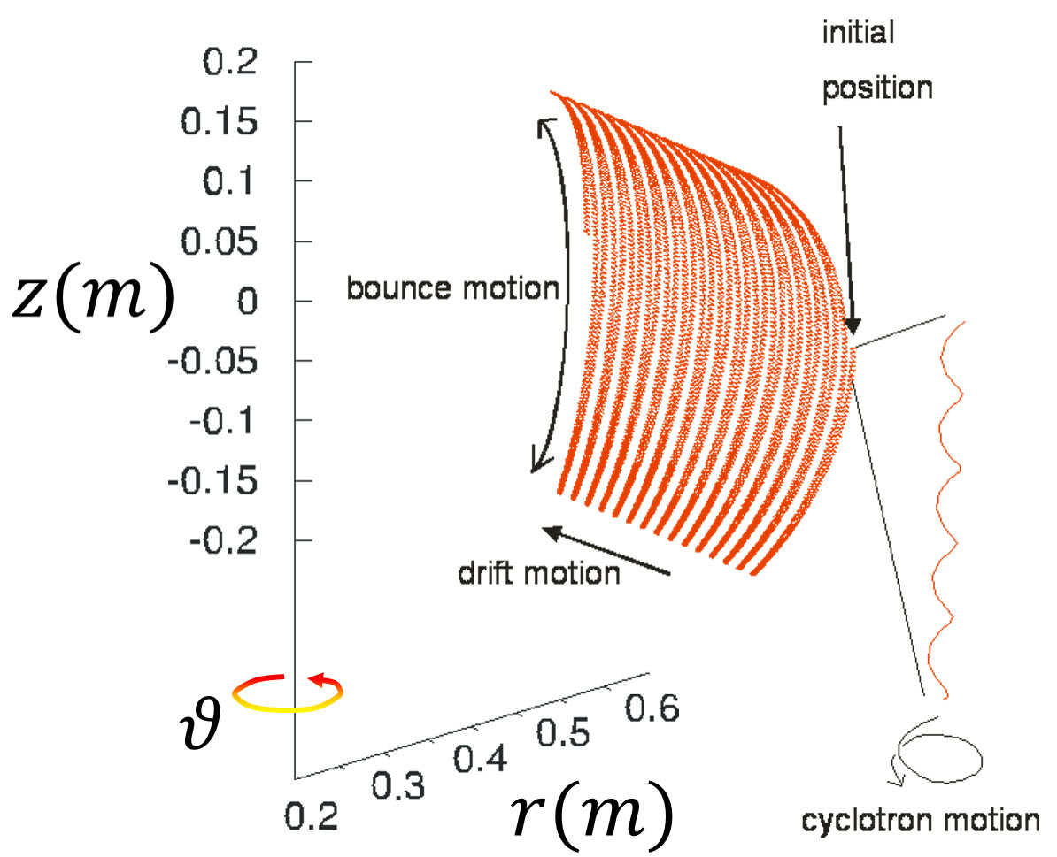
Figure 1: A typical orbit of a magnetized particle in a dipole magnetic field, which has a hierarchy of three different frequencies. Here we assume the parameters of the RT-1 device yoshida2010 ; the magnetic field at the confinement region is about 0.05T. For a particle having an isotropic energy of 50eV, $\omega_{c}\sim$ 1GHz, $\omega_{b}\sim$ 1MHz, and $\omega_{d}\sim$ 1kHz.

We define the “relaxed state” by a distribution function $f$ that has no $\psi$ dependence, i.e.,

$$\frac{\partial f}{\partial\psi}=0.$$ (1)

For the equilibrium to be non-trivial, we demand that the total canonical angular momentum $\int\psi fd^{6}z$ to be a non-zero constant ($d^{6}z$ denotes the volume element of the phase space).

II Kinetic model of macroscopic relaxed sate

In order to formulate the model with taking into account the hierarchy of adiabatic invariants, we write the Hamiltonian of a particle as

$$H_{gc}=\omega_{c}\mu+\omega_{b}J_{\parallel}+q\phi.$$ (2)

We have omitted the kinetic energy $(P_{\theta}-q\psi)^{2}/(2mr^{2})$ of the toroidal drift velocity by approximating $P_{\theta}=q\psi$ drift_kinetic . By the symmetry, the toroidal angle $\theta$ is not included in $H_{gc}$. The gyro angle ${\vartheta_{c}}$ (which is conjugate to the magnetic moment $\mu$) is coarse-grained by replacing $\dot{\vartheta_{c}}$ with $\omega_{c}$, and is completely eliminated from $H_{gc}$ (i.e., $H_{gc}$ dictates the motion of the guiding center of the gyrating particle). However, the bounce angle ($\vartheta_{b}$) is not ignored, because the frequencies $\omega_{c}$ and $\omega_{b}$, as well as the electric potential $\phi$ are functions of the spacial coordinates including $\vartheta_{b}$. Here we choose $\psi$ and $\zeta$ (the parallel coordinate along each magnetic surface, the level-set of $\psi$) as the spatial coordinates (then, $\vartheta_{b}=\pi\zeta/\ell_{\parallel}$; $\ell_{\parallel}$ is the bounce orbit length).

The action $J_{\parallel}$ is conjugate to $\vartheta_{b}$:

$$\dot{J}_{\parallel}=\frac{\partial H_{gc}}{\partial\vartheta_{b}}=\frac{\ell_{\parallel}}{\pi}\frac{\partial H_{gc}}{\partial\zeta}.$$ (3)

For the periodic bounce motion, $\oint(\partial H_{gc}/\partial\vartheta_{b})d\vartheta_{b}=\oint dH_{gc}=0$. Integrating (3) over the cycle of bounce motion yields the bounce-average $\langle J_{\parallel}\rangle=$ constant. When we calculate macroscopic quantities (like the total energy or the total action), we evaluate $J_{\parallel}$ as the adiabatic invariant $\langle J_{\parallel}\rangle$.

The drift frequency (including all grad-B, curvature, and E$\times$B drifts) is given by bounce-averaging the toroidal angular velocity

$$\omega_{d}=\dot{\theta}=\frac{\partial H_{gc}}{\partial\psi}=\mu\frac{\partial\omega_{c}}{\partial\psi}+J_{\parallel}\frac{\partial\omega_{b}}{\partial\psi}+q\frac{\partial\phi}{\partial\psi}.$$ (4)

In a homogeneous magnetic field, both $\omega_{c}$ and $\omega_{b}$ are constant, and then (4) evaluates the E$\times$B drift frequency.

In terms of the constants of motion $H_{gc}$, $\mu$, $J_{\parallel}$, and $\psi$, a general equilibrium solution of the drift kinetic equation (such that $\{H_{gc},f\}=0$) is written as $f(H_{gc},\mu,J_{\parallel},\psi)$. The relaxed state is the special solution that maximizes the entropy $S=-\int f\log f\,d^{6}z$ under the constraints on

1. the total particle number $N=\int f\,d^{6}z$,

2. the total energy $E=\int H_{gc}f\,d^{6}z$,

3. the total magnetic moment $C_{\mu}=\int\mu f\,d^{6}z$,

4. the total bounce action $C_{J_{\parallel}}=\int J_{\parallel}f\,d^{6}z$,

5. the total angular momentum $C_{\psi}=\int\psi f\,d^{6}z$.

The variational principle yields

$$f_{T}(H_{gc},\mu,J_{\parallel},\psi)=Z^{-1}e^{-\beta(H_{gc}-\gamma_{1}\mu-\gamma_{2}J_{\parallel}-\gamma_{3}\psi)},$$ (5)

where $Z$ (normalization factor), $\beta$ (inverse temperature), $\gamma_{1}$, $\gamma_{2}$, and $\gamma_{3}$ are constants related to the Lagrange multipliers on $N$, $E$, $C_{\mu}$, $C_{J_{\parallel}}$, and $C_{\psi}$.

While we derived (5) for a given set of constants, we may, alternatively, regard $f_{T}$ as a Boltzmann distribution on a grand-canonical ensemble parametrized by the aforementioned macroscopic quantities, and then, we interpret $\gamma_{1},\gamma_{2}$ and $\gamma_{3}$ as the chemical potentials pertinent to the changes in the action variables $\mu$, $J_{\parallel}$, and $\psi$, respectively (remember the parallel relations between the “energy level” and the frequency, as well as between the “particle number” and the action variable, in analogy with the Landau levels in quantum theory).

Finally, the determining equation (1) must be satisfied, which is equivalent to

$$\frac{\partial H_{gc}}{\partial\psi}=\gamma_{3}~{}(=\textrm{constant}).$$ (6)

Remembering (4), we find that (6) implies rigid rotation.

The relaxed-state plasma occupies a finite domain that is surrounded by a magnetic surface, i.e., we can connect the distribution function $f_{T}$ to the vacuum $f=0$ at some level-set $\psi=\psi^{*}$. Invoking Heaviside’s step function $Y(\psi^{*}-\psi)$ (which is zero inside the plasma region), we may write the extended distribution function as

$$\tilde{f}_{T}(H_{gc},\mu,J_{\parallel},\psi)=\lim_{\alpha\rightarrow\infty}e^{-\alpha Y(\psi^{*}-\psi)}\cdot f_{T},$$ (7)

which is in equilibrium ($\{H_{gc},\tilde{f}_{T}\}=0$) and relaxed: $\partial\tilde{f}_{T}/\partial\psi=0$ except at the boundary (the boundary is not “relaxed” as it reflects the constraint given by $C_{\psi}$; later, we will show how the boundary is determined).

Neglecting the current generated by the plasma, $\psi$ is a given function. Then, (6) may be viewed as a determining equation for the electric potential $\phi$ (in addition to the term $q\phi$, $J_{\parallel}$ depends on $\phi$ in a complex way; however, if the electric field is much stronger than the thermal energy, we may approximate $\bm{B}\cdot\nabla\phi\approx 0$, and then, $J_{\parallel}$ is independent to $\phi$, and we may put $\phi=\phi(\psi)$).

The electric potential $\phi$ included in $H_{gc}$ must be consistent to the field equation

$$-\nabla^{2}\phi =4\pi q\rho,$$ (8a)

$$\rho =\int f_{T}(\bm{x},\bm{v})\,d^{3}v=\int f_{T}\,\frac{2\pi\omega_{c}d\mu}{m}\frac{dJ_{\parallel}}{m\ell_{\parallel}}.$$ (8b)

The existence of a self-consistent field $\phi$ satisfying both (6) and (8a) is not at all obvious. In what follows, we will construct non-trivial solutions; one is the well-known “thermal equilibrium” in a straight homogeneous magnetic field, and the other is a new solution (numerical) in a dipole magnetic field.

III Thermal equilibrium in a homogeneous magnetic field

First, we put the classical solution into the new perspective formulated here. In a homogeneous longitudinal magnetic field $\bm{B}=B_{0}\nabla z$ ($B_{0}$ is a constant), $\omega_{c}$ and $\omega_{b}$ are constants. We may put $\psi=B_{0}r^{2}/2$ and $\phi=\phi(\psi)$ (assuming that the relaxed state is homogeneous with respect to $\zeta=z$). The relaxed-state condition (1) reads $q\partial\phi/\partial\psi=\gamma_{3}$, which yields $\phi=(\gamma_{3}/q)\psi$, and

$$f_{T}=Z^{-1}e^{-\beta[(\omega_{c}-\gamma_{1})\mu+(\omega_{b}-\gamma_{2})J_{\parallel}]}.$$ (9)

Since this distribution function has no spatial dependence, $\rho=\rho_{0}$ (constant). On the field equation (8a), the potential $\phi=(\gamma_{3}/q)\psi=(\gamma_{3}/q)B_{0}r^{2}/2$ is consistent to the flat density $\rho_{0}$, if $\gamma_{3}=-2\pi q^{2}\rho_{0}/B_{0}=-\omega_{p}^{2}/(2c\omega_{c})$. The parameter $\gamma_{3}$ controls the density $\rho_{0}$ (while $\gamma_{1}$ and $\gamma_{2}$ change the velocity anisotropy). Given the particle number $N$ (per unit length in $z$), $\rho_{0}=N/(\pi R^{2})$, where $R$ is the radius of the plasma column. The total angular momentum evaluates $C_{\psi}=B_{0}NR^{2}/4$. Hence, for given $N$ and $C_{\psi}$, we obtain $R=2\sqrt{C_{\psi}/B_{0}N}$.

IV Relaxed state in a dipole magnetic field

In a dipole magnetic field, both $\omega_{c}$ and $\omega_{b}$ vary as functions of the spacial coordinates $\psi$ and $\zeta$. Because of the inhomogeneous Jacobian weight in the integral (8b), the parameters $\gamma_{1}$ and $\gamma_{2}$, included in $f_{T}$, cause a change in the profile of $\rho$ hasegawa2005 ; yoshida2013 , which is in marked contrast to the foregoing case of homogeneous magnetic field.

Assuming some $\phi$ in $f_{T}$, we calculate $\rho$ by (8b), and then solve (8a) for a new $\phi$. Iterating this process, we obtain a self-consistent $\phi$ and a kinetic equilibrium $f_{T}$. Next we have to vary the parameters $\gamma_{1}$, $\gamma_{2}$, and $\gamma_{3}$ to find the relaxed state.

Since the left-hand side of (6) contains $\mu$ and $J_{\parallel}$, we cannot satisfy (6) for each particle having different $\mu$ and $J_{\parallel}$ (excepting the case when $\partial\omega_{c}/\partial\psi=\partial\omega_{b}/\partial\psi=0$, as it is in a homogeneous magnetic field). Instead, we demand that the macroscopic drift velocity

$$\overline{v}_{\theta}=\rho^{-1}\int v_{\theta}f_{T}\frac{2\pi\omega_{c}}{m}d\mu dv_{\parallel}$$ (10)

is rigid rotation ($v_{\theta}$ is directly evaluated by the orbit calculations). The chemical potentials $\gamma_{1},\gamma_{2}$, and $\gamma_{3}$ are the control parameters to be optimized to yield rigid rotation.

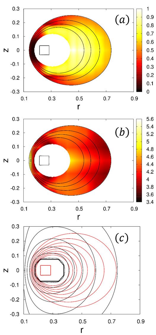
Figure 2: A relaxed state in a dipole magnetic field: (a) self-consistent density profile $\rho$, (b) the distribution of the angular velocity $\omega_{d}$, and (c) the contours of the electric potential $\phi$ (black lines) and the magnetic flux function $\psi$ (the magnetic field lines; red lines).

Figure 2 shows an example of solution. Here we assume parameters that simulate the RT-1 experiment yoshida2010 . The temperature $\beta^{-1}=50$eV is chosen to be the typical energy of the injected electrons. Other parameters are $(\gamma_{1},\gamma_{2},\gamma_{3})=(-8.0\times 10^{-2}\,T,-7.2\times 10^{6}\,s^{-1},\,1.4\times 10^{4}\,Wb^{-1}\,eV)$, by which $\beta\gamma_{1}\mu$, $\beta\gamma_{2}J_{\parallel}$, $\beta\gamma_{3}\psi$, and $\beta q\phi$ are all of order $\beta H\sim 1$ (implying that all terms in $f_{T}$ play essential roles in characterizing the relaxed state).

V Numerical analysis

Here we study how general equilibrium solutions (consistent $\phi$ and $f_{T}$ satisfying $\{H_{gc},f_{T}\}=0$ and the Poisson equation (8a) simultaneously) vary as the parameters are changed, and how these parameters can be optimized to send the equilibrium to the relaxed state.

For the convenience, we introduce indexes to evaluate the “relaxation”:

$$\bar{\omega}_{d}=\frac{1}{N}\int{\omega_{d}\rho d^{3}x},$$ (11a)

$$\sigma_{\omega_{d}}=\sqrt{\frac{1}{N}\int{\left(\omega_{d}-\bar{\omega}_{d}\right)^{2}\rho d^{3}x}},$$ (11b)

$$\chi=\frac{\sigma_{\omega_{d}}}{\bar{\omega}_{d}},$$ (11c)

i.e., $\bar{\omega}_{d}$ the spatially averaged toroidal drift frequency, $\sigma_{\omega_{d}}$ the associated standard deviation, and $\chi$ a measure of rigidity of the rotation.

In Fig. 3, the behavior of $\chi$ as a function of the control parameters $\gamma_{1}$, $\gamma_{2}$, $\gamma_{3}$, and $\phi_{0}$ (the electric potential at the coil surface) is shown. A detailed explanation for each parameter is given in the following subsections.

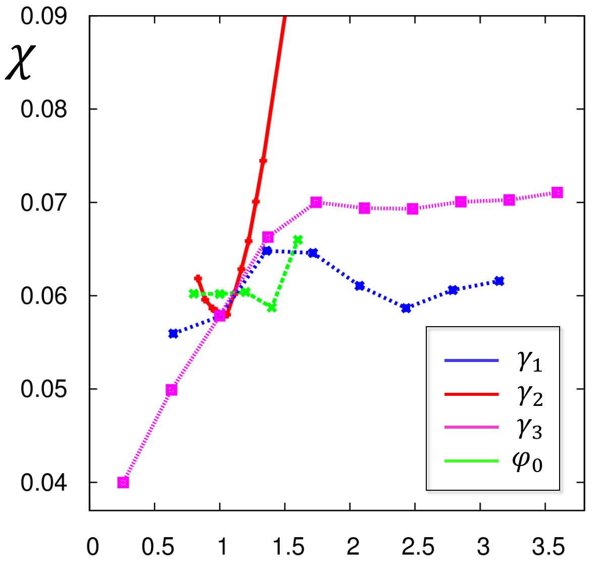
Figure 3: The rigidity parameter $\chi$ as functions of $\gamma_{1}$, $\gamma_{2}$, $\gamma_{3}$ and $\phi_{0}$. Each parameter is normalized by the corresponding central value $(\gamma_{1},\gamma_{2},\gamma_{3},\phi_{0})=(-8.0\times 10^{-2}\,T,-7.2\times 10^{6}\,s^{-1},\,1.4\times 10^{4}\,Wb^{-1}\,eV,-250\,V)$, and changed independently.

V.1 Chemical potential $\gamma_{1}$ of the magnetic moment $\mu$

The dependence of the equilibrium state on the parameter $\gamma_{1}$ (the chemical potential of the magnetic moment $\mu$) is shown in Figs. 4 (plots of $\omega_{d}$) and 5 (plots of $\rho$). Here, other parameters are fixed at $\phi_{0}=-250\,V$, $\beta^{-1}=50$eV, and $(\gamma_{2},\gamma_{3})=(-0.72\times 10^{7}s^{-1},1.25\times 10^{4}\,Wb^{-1}\,eV)$. As $\gamma_{1}$ is increased, the density approaches to the distribution $\rho\propto B$ yoshida2013 . However, the rigidity of the rotation is a weak function of $\gamma_{1}$ (see Fig. 3).

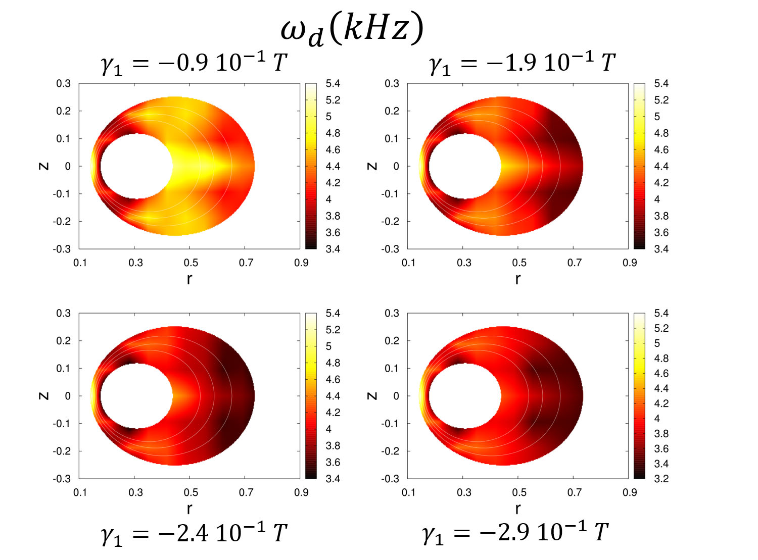
Figure 4: Plots of the angular frequency $\omega_{d}(kHz)$ of rotation for four different values of $\gamma_{1}(T)$.

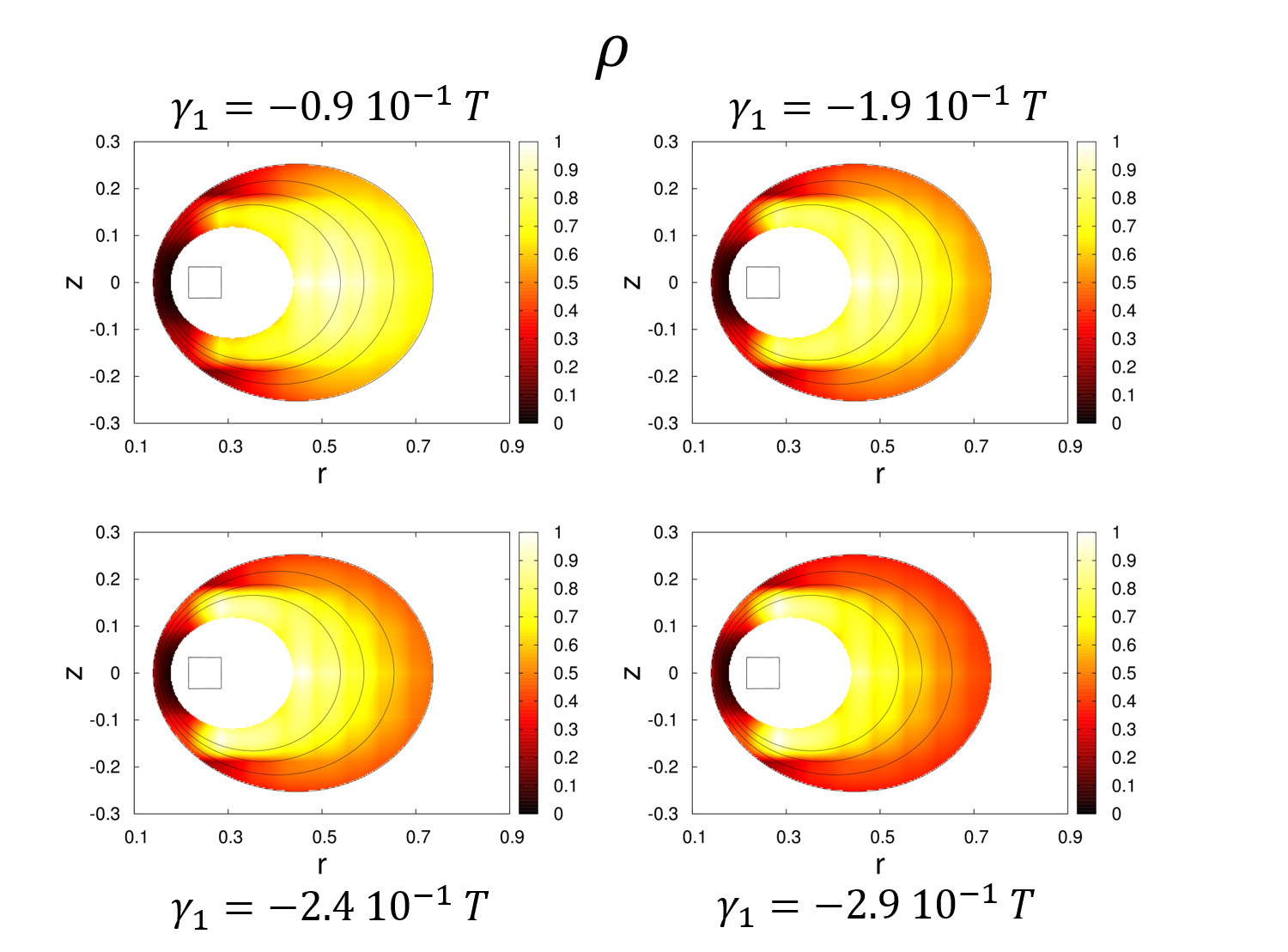
Figure 5: Plots of the density $\rho$ (normalized) for four different values of $\gamma_{1}(T)$.

V.2 Chemical potential $\gamma_{2}$ of the bounce action $J_{\parallel}$

The chemical potential $\gamma_{2}$ of the bounce action $J_{\parallel}$ has a rather strong influence on the equilibrium distribution; see Figs. 6 (plots of $\omega_{d}$) and 7 (plots of $\rho$). With the optimum value $\gamma_{2}=0.7\times 10^{7}\,s^{-1}$, the density $\rho$ has a broad distribution with a highly homogeneous drift frequency $\omega_{d}$. However, when $\gamma_{2}$ is increased, the density profile shrinks to a disk-like shape with a strong shear in $\omega_{d}$. Here, other parameters are fixed at $\phi_{0}=-250\,V$, $\beta^{-1}=50$eV, and $(\gamma_{1},\gamma_{3})=(-0.795\times 10^{-1}\,T,1.25\times 10^{4}\,Wb^{-1}\,eV)$. The change of $\chi$ as a function of $\gamma_{2}$ is given in Fig. 3.

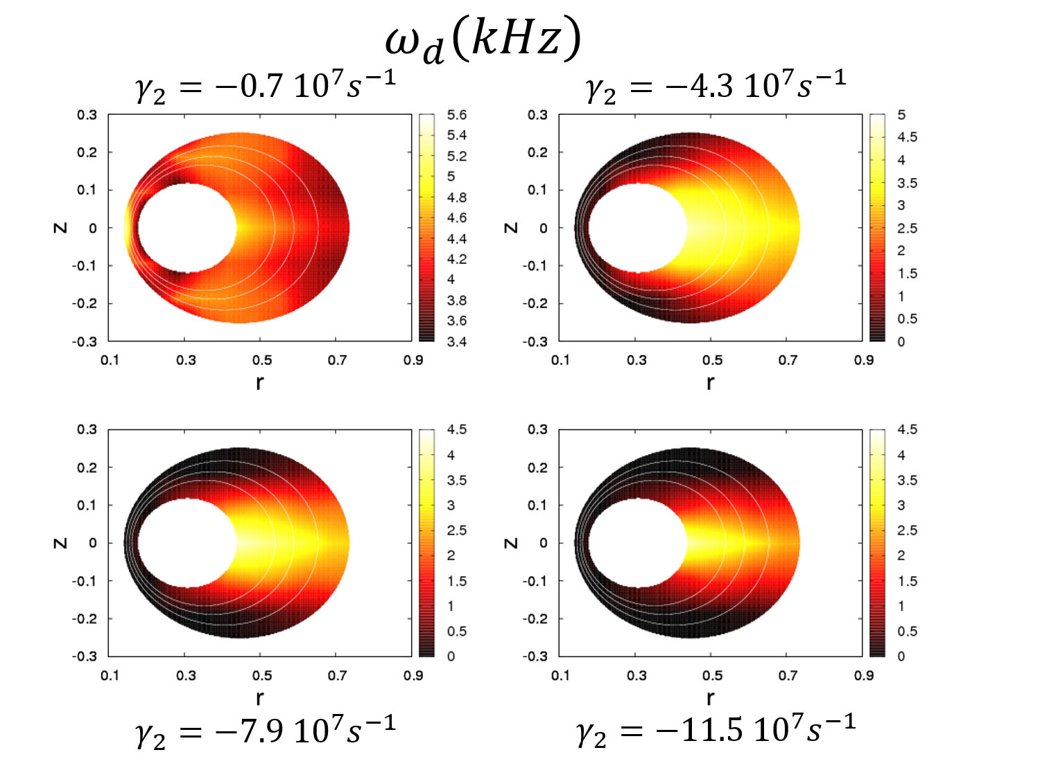
Figure 6: Plots of the angular frequency $\omega_{d}(kHz)$ of rotation for four different values of $\gamma_{2}(s^{-1})$.

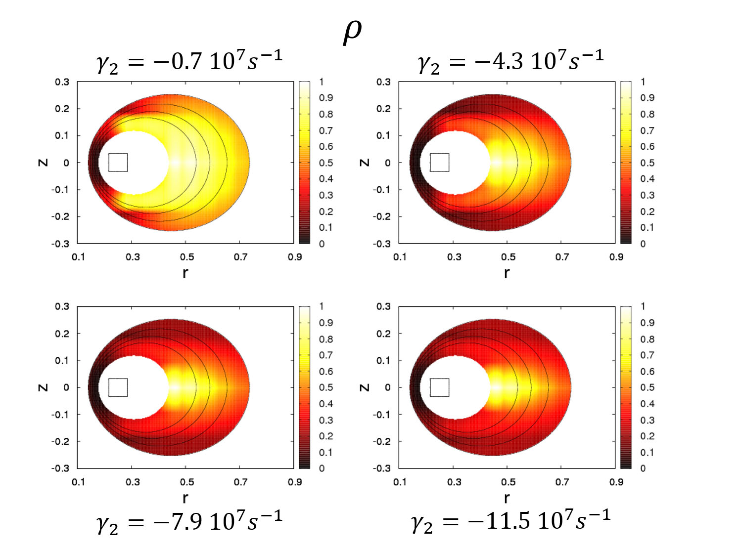
Figure 7: Plots of the density $\rho$ (normalized) for four different values of $\gamma_{2}(s^{-1})$.

V.3 Chemical potential $\gamma_{3}$ of the angular momentum $\psi$

The chemical potential $\gamma_{3}$ of the angular momentum $\psi$ also has a strong influence on the equilibrium; see Figs. 8 (plots of $\omega_{d}$) and 9 (plots of $\rho$). As $\gamma_{3}$ is increased, the distribution function becomes $f\approx e^{\beta(\gamma_{3}\psi-q\phi)}$, and then the drift frequency scales as $\omega_{d}\sim r^{-1}$, since $\omega_{d}=q\partial\phi/\partial\psi$ and, at $z=0$, $\psi\sim r^{-1}$ and $\phi\sim r^{-2}$ (if we assume a constant particle number per flux tube volume hasegawa2005 , $\rho\sim r^{-4}$ which gives $\Delta\phi\sim r^{-4}$). Here, other parameters are fixed at $\phi_{0}=-250\,V$, $\beta^{-1}=50$eV, and $(\gamma_{1},\gamma_{2})=(-0.795\times 10^{-1}\,T,-0.72\times 10^{7}\,s^{-1})$. The change of $\chi$ as a function of $\gamma_{3}$ can be found in Fig. 3.

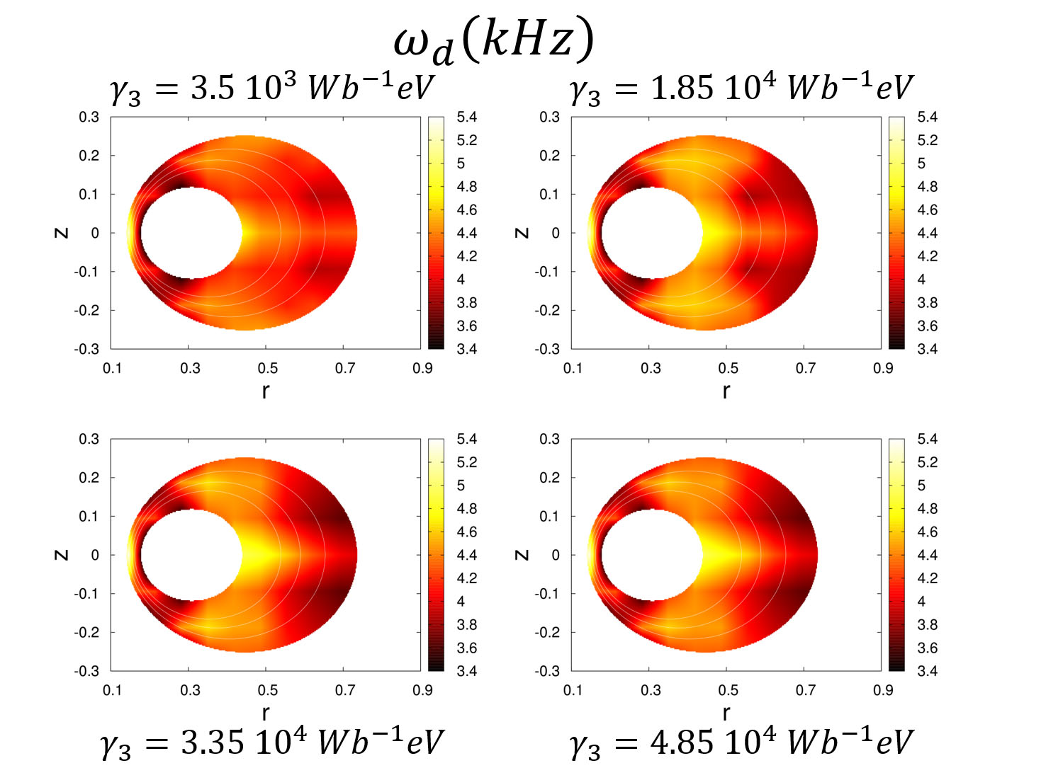
Figure 8: Plots of the angular frequency $\omega_{d}(kHz)$ of rotation for four different values of $\gamma_{3}(Wb^{-1}\,eV)$.

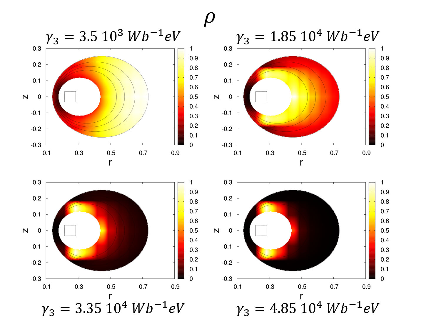
Figure 9: Plots of the density $\rho$ (normalized) for four different values of $\gamma_{3}(Wb^{-1}\,eV)$.

V.4 Inner boundary potential $\phi_{0}$

In addition to the four parameters $\beta$, $\gamma_{1}$, $\gamma_{2}$, and $\gamma_{3}$, there is another important parameter $\phi_{0}$ that is the boundary value of the potential $\phi$ at the surface of the internal magnet. By changing $\phi_{0}$, the confinement is dramatically improved; see the experimental result reported in Saitoh2004 . On the levitated magnet experiment yoshida2010 , however, $\phi_{0}$ is spontaneously determined, because the coil surface is floating. Figures 10 and 11, respectively, show the distribution of the drift frequency $\omega_{d}$ and the density $\rho$ for four different values of $\phi_{0}$. Other parameters are fixed at $\beta^{-1}=50$eV and $(\gamma_{1},\gamma_{2},\gamma_{3})=(-0.795\times 10^{-1}\,T,-0.8\times 10^{7}s^{-1},1.35\times 10^{4}\,Wb^{-1}\,eV)$. Interestingly, as $\phi_{0}$ changes, the confinement region (the density clump) moves, while the rigidity of the rotation is not influenced by $\phi_{0}$; see Fig. 3.

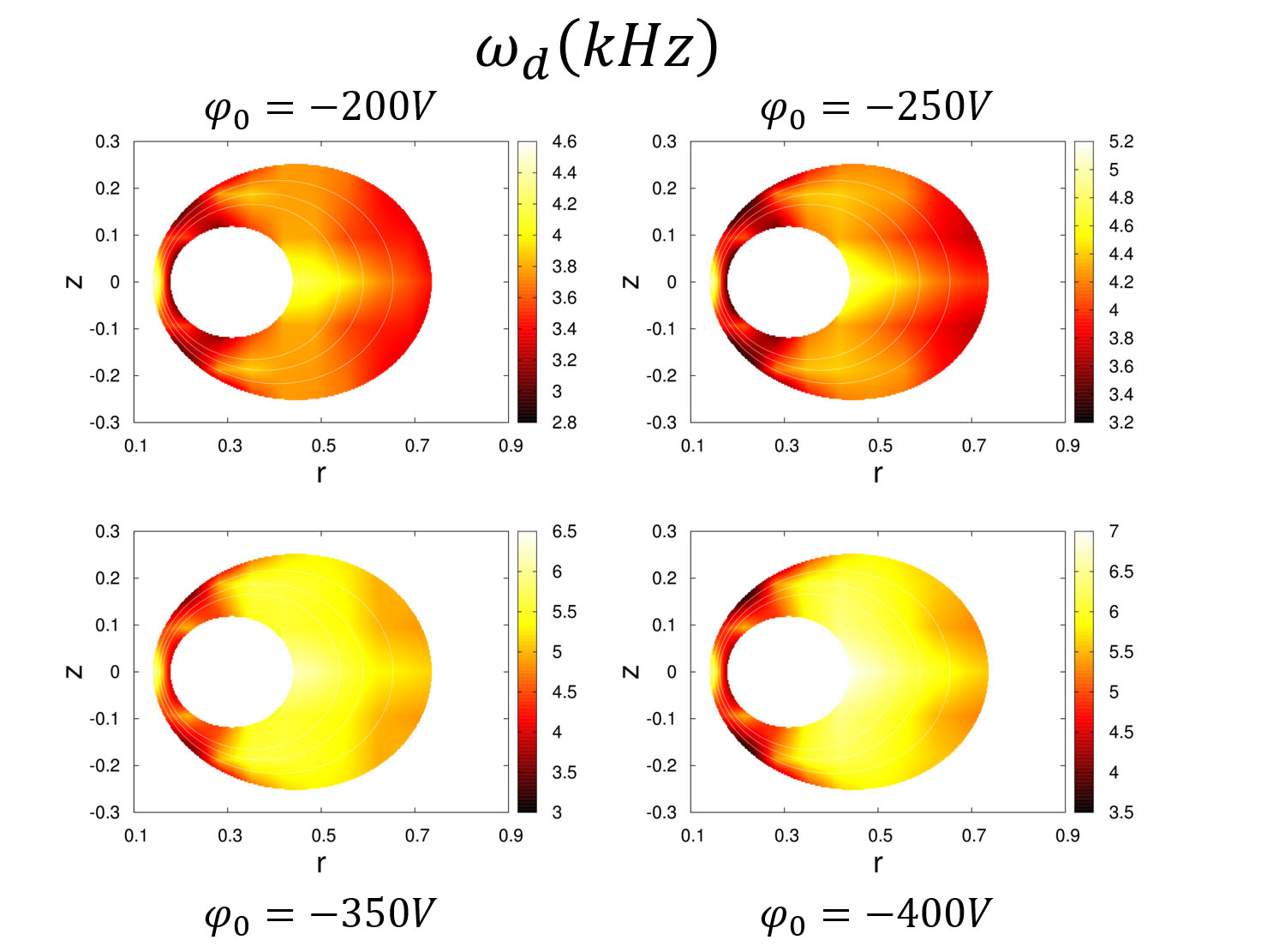
Figure 10: Plots of the angular frequency $\omega_{d}(kHz)$ of rotation for four different values of $\phi_{0}(V)$.

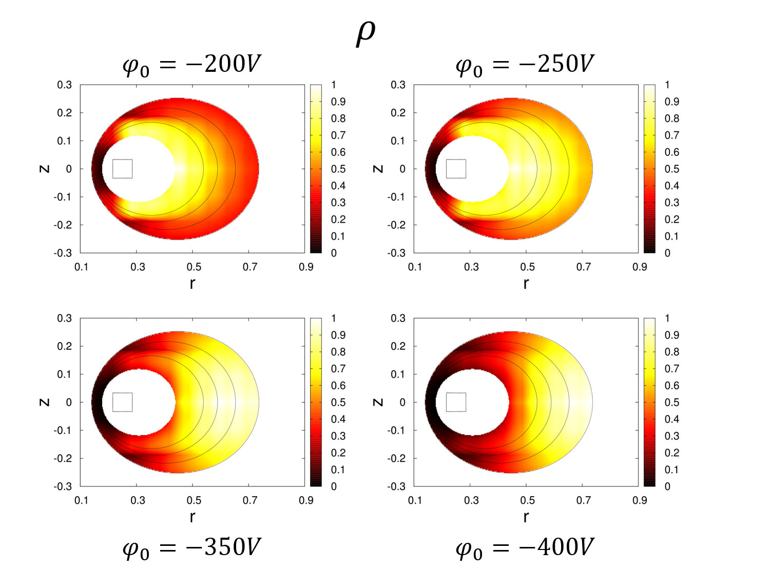
Figure 11: Plots of the density $\rho$ (normalized) for four different values of $\phi_{0}(V)$.

VI Conclusion

Putting a classical knowledge into a wider perspective, a deeper principle may emerge; here we have described such an example of paradigm shift in the study of the relaxed state (or, thermal equilibrium) of charged particles. Formulating a relaxed state on a topologically constrained macroscopic phase space, we have found that a rigidly-rotating equilibrium can self-organize even in an inhomogeneous magnetic field. In an experimental system, tuning of the parameters $\gamma_{1},\gamma_{2},\gamma_{3}$, and $\phi_{0}$ occurs spontaneously through the relaxation process. Among them, $\gamma_{2}$ and $\gamma_{3}$ influence strongly on the profile of $\omega_{d}$. Whereas we formulated the equilibrium assuming that the corresponding $C_{J_{\parallel}}$ and $C_{\psi}$ are given (then, the Lagrange multipliers $\gamma_{2}$ and $\gamma_{3}$ are determined by prescribed $C_{J_{\parallel}}$ and $C_{\psi}$), the plasma may change them (by dissipating the constants of motion) in order to relax into the thermal equilibrium; the self-organization is a process that selects optimum $C_{J_{\parallel}}$ and $C_{\psi}$ (hence, $\gamma_{2}$ and $\gamma_{3}$). In fact, these two actions are relatively “fragile” with respect to the other constant $C_{\mu}$.

The present model of relaxed states differs from the previously formulated Boltzmann distribution of a neutral plasma yoshida2013 , which is created by constraining only $C_{\mu}$ and $C_{J_{\parallel}}$ (in addition to the standard constraints $N$ and $E$) in maximizing the entropy; freeing $C_{\psi}$ means that $\psi$ is not a conserved quantity. In the present formulation, however, we also constrain $C_{\psi}$, while we demand $\partial f/\partial\psi=0$ as the criteria of the relaxed state. The latter is a weaker criterion, i.e., the present solution is not necessarily the maximum entropy state of the former setting, as far as $\psi$ is freed from the kinetic energy (i.e., we omit the energy of the drift velocity) and is deemed as a spatial coordinate variable. This is obvious by putting $\gamma_{3}$ (the Lagrange multiplier on $C_{\psi}$) $=0$ in the thermal equilibrium (9). Then, the solution becomes $\omega_{d}\rightarrow 0$, $\rho\rightarrow 0$ with $\beta q\phi\rightarrow$ constant ($=\infty$), i.e., the radius of the plasma column diverges, implying no confinement.. The constraint on the total angular momentum $C_{\psi}$ yields a finite radius of confinement.

References

- (1) D. Lynden-Bell and R. Wood, Mon. Not. R. Astron. Soc. 138, 495 (1968).
- (2) M. Schulz and L. J. Lanzerotti, Particle Diffusion in the Radiation Belts (Springer, New York, 1974).
- (3) A. C. Boxer et al., Nature Phys. 6, 207 (2010).
- (4) Z. Yoshida et al., Plasma Phys. Control. Fusion 55, 014018 (2013).
- (5) D. H. E. Dubin and T. M. O’Neil, Rev. Mod. Phys. 71, 87 (1999).
- (6) A. Antoniazzi, D. Fanelli, S. Ruffo, and Y. Y. Yamaguchi. Phys. Rev. Lett. 99, 040601 (2007).
- (7) R. Pakter and Y. Levin, Phys. Rev. Lett. 106, 200603 (2011).
- (8) P. J. Morrison, Rev. Mod. Phys. 70, 467 (1998).
- (9) Z. Yoshida and S. M. Mahajan, Prog. Theor. Exp. Phys. 2014, 073J01 (2014).
- (10) J. H. Malmberg and J. S. de Grassie, Phys. Rev. Lett. 35, 577 (1975).
- (11) J. H. Malmberg and C. F. Driscoll, Phys. Rev. Lett. 44, 654 (1980).
- (12) Z. Yoshida, H. Saitoh, J. Morikawa, Y. Yano, S. Watanabe and Y. Ogawa, Phys. Rev. Lett. 104, 235004 (2010).
- (13) H. Saitoh et al., Phys. Plasmas 17, 112111 (2010).
- (14) Z. Yoshida et al., in Non-Neutral Plasma Physics III, AIP Conf. Proceedings No. 498 (AIP, New York, 1999), p. 397
- (15) T. S. Pedersen and A. H. Boozer, Phys. Rev. Lett. 88, 205002 (2002).
- (16) T. S. Pedersen et al., J. Phys. B: At. Mol. Opt. Phys. 36, 1029 (2003).
- (17) A.J. Lichtenberg and M.A. Lieberman, Regular and Chaotic Dynamics, 2nd ed. (Springer-Verlag, New York, 1992), Sec. 1.3d.
- (18) There is a subtlety in the representation of the energy of the drift velocity; see J. R. Cary and A. J. Brizard, Rev. Mod. Phys. 81, 693 (2009). Whereas we omit the energy of the drift velocity, we still have a drift velocity; see (4).
- (19) A. Hasegawa, Phys. Scr. T116, 72 (2005).
- (20) H. Saitoh et al., Phys. Rev. Lett. 92, 255005 (2004).