A novel method for identifying exoplanetary rings

Abstract

The discovery of rings around extrasolar planets (“exorings”) is one of the next breakthroughs in exoplanetary research. Previous studies have explored the feasibility of detecting exorings with present and future photometric sensitivities by seeking anomalous deviations in the residuals of a standard transit light curve fit, at the level of $\simeq 100$ ppm for Kronian rings. In this work, we explore two much larger observational consequences of exorings: (1) the significant increase in transit depth that may lead to the misclassification of ringed planetary candidates as false-positives and/or the underestimation of planetary density; and (2) the so-called “photo-ring” effect, a new asterodensity profiling effect, revealed by a comparison of the light curve derived stellar density to that measured with independent methods (e.g., asteroseismology). While these methods do not provide an unambiguous detection of exorings, we show that the large amplitude of these effects combined with their relatively simple analytic description, makes them highly suited to large-scale surveys to identify candidate ringed planets worthy of more detailed investigation. Moreover, these methods lend themselves to ensemble analyses seeking to uncover evidence of a population of ringed planets. We describe the method in detail, develop the basic underlying formalism and test it in the parameter space of rings and transit configuration. We discuss the prospects of using this method for the first systematic search of exoplanetary rings in the Kepler database and provide a basic computational code for implementing it.

1. Introduction

Since the discovery of the first transiting planet (Charbonneau et al. 2000; Henry et al. 2000), planetary eclipses have emerged as powerful tools for characterizing exoplanets. Numerous novel methods have been devised using transits to identify non-conventional planetary properties, such as oblateness (Carter & Winn 2010; Leconte et al. 2011), magnetic bow shocks (Vidotto et al. 2010), exomoons (Kipping 2009; Heller et al. 2014), and exoplanetary rings or “exorings” (Barnes & Fortney 2004; Ohta et al. 2009; Tusnski & Valio 2011; Mamajek et al. 2012; Kenworthy & Mamajek 2015).

With the advent of new instruments surveying the sky for transits with precise photometry (PLATO, Rauer & Catala 2011; EELT, Guyon et al. 2012; GMT, Johns et al. 2012; TESS, Ricker et al. 2014 and JWST, Beichman et al. 2014), there is great potential for discoverying new and unconventional exoplanetary phenomena in the coming decade.

The discovery of exorings would be particularly interesting. All of the solar system’s giant planets have rings and at least one, Saturn, has sufficiently extended ring systems that are sufficiently extended to produce observable signatures with current/future instrumentation (Barnes & Fortney 2004; Ohta et al. 2009). The discovery and characterizarion of exorings could shed light on important planetary processes, such as planetary and moon formation (Mamajek et al. 2012) and planetary interior structure (Schlichting & Chang 2011).

Barnes & Fortney (2004) developed the first theoretical model of exoring transits. They showed that, provided photometric sensitivities and time resolution of $1-3\times 10^{-4}$ and $\sim$ 15 minutes, light curve residual analysis could be used to resolve and characterize rings. More recently, Ohta et al. (2009) showed that the presence of rings could produce spectroscopic signatures, detectable by ground-based telescopes, for sensitivities $<0.1$ m $s^{-1}$. Independently, Tusnski & Valio (2011) have tested a model of ring transits showing that the properties of hypothetical rings can be reliably recovered.

Despite these theoretical advances, there have been no systematic surveys for exorings with archival photometry. One reason for this is the assumption that a practical ring survey would employ the same technique as that for their discovery and characterization, namely, the detailed analysis of light curves via fits to complex ring transit models.

Here, we present a novel method for perfoming systematic searches for exoring candidates. Our method relies only on the measurement of the basic transit parameters (i.e. depth, duration), avoiding the need for computationally expensive fits of a transit ring model. The method exploits simple analytical formulae and hence is well-suited for performing searches in large photometric databases.

2. Ring transit geometry

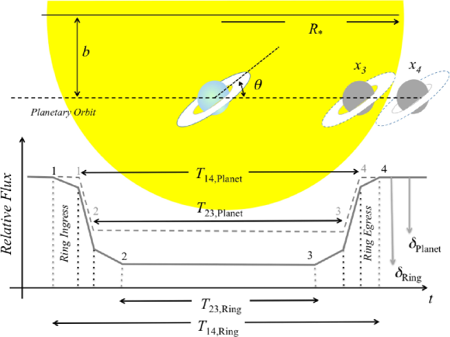
Figure 1.— Schematic ring and planetary transit geometry and light curve. Sizes are not at scale. Transit depth ($\delta$) and total duration ($T_{14}$) are larger when an exoring is present, whereas the duration of full transit ($T_{23}$) is lower.

One of the most powerful properties of planetary transits is the wealth of information they can provide by simply monitoring variations in stellar brightness.

Assuming that the transiting object is spherical and other conventional conditions, Seager & Mallén-Ornelas (2003) showed that the planetary radius $p\equiv R_{\rm p}/R_{\star}$, scaled orbital semimajor axis, $a/R_{\star}$, and impact parameter, $b$, can be derived from three basic observables:

• transit depth, $\delta=(F_{\rm o}-F)/F_{\rm o}$ (where $F$ and $F_{\rm o}$ represent the in-transit and out-of-transit stellar fluxes, respectively);

• first-to-fourth contact transit duration, $T_{\rm 14}$;

• second-to-third contact transit duration, $T_{\rm 23}$.

Figure 1 schematically depicts the definition of these quantities and the significant differences imposed by the presence of planetary rings.

Our basic ring transit model relies on three basic assumptions.

• The planet and the star are spherical.

• Rings are uniform and scatter/absorb light only between radii $R_{\rm i}=f_{\rm i}R_{\rm p}$ and $R_{\rm e}=f_{\rm e}R_{\rm p}$ (constant normal optical depth $\tau$).

• Diffractive forward scattering in ring particles does not modify the basic transit parameters (Barnes & Fortney 2004).

Under these assumptions, the transit depth of a ringed planet is given by the ratio:

$$\delta=\frac{A_{\rm Rp}}{A_{\star}}=\frac{A_{\rm Rp}}{\pi R_{\star}^{2}},$$ (1)

where $A_{\rm Rp}$ and $A_{\star}$ are the effective projected ring-planet and stellar area.

The ring area is computed with the analytical expression (see Appendix A for details)

$$A_{\rm Rp}=\pi R_{p}^{2}+\pi[r^{2}(f_{\rm e})-r^{2}(f_{\rm i})]\,R_{p}^{2},$$ (2)

where $r$ is the effective ring radius and is given by

$$r^{2}(f)=\beta(\cos i_{\rm R})\times\;\left\{\begin{array}[]{ll}\scriptstyle f^{2}\cos i_{\rm R}-1&\scriptstyle f\cos i_{\rm R}>1\\ \begin{array}[]{ll}\scriptstyle f^{2}\cos i_{\rm R}&\frac{2}{\pi}{\scriptstyle\rm arcsin}\scriptstyle(y)+\\ \scriptstyle-&\frac{2}{\pi}{\scriptstyle\rm arcsin}\scriptstyle(yf\cos i_{\rm R})\end{array}&\scriptstyle{\rm otherwise}\end{array}\right..$$ (3)

Here, $i_{\rm R}$ is the projected ring inclination ($i_{\rm R}=90^{\circ}$ if the ring is edge on) and $y=\sqrt{f^{2}-1}/(f\sin i_{\rm R})$ is an auxiliary variable. The term $\beta(\cos i_{\rm R})\equiv 1-e^{-\tau/\cos i_{\rm R}}$ accounts for the ring’s effective absortion of stellar light (Barnes & Fortney 2004).

To calculate ring transit durations, $T_{\rm 14}$ and $T_{\rm 23}$, we need to compute the planet center horizontal coordinate, $x$, where the the external ring or the planetary disk intersects the stellar limb at a single point (see Figure 1). Four $x$ values, the contact positions, $x_{i}$ ($i=1,2,3,4$), fulfill this condition.

In the case of a non-ringed spherical planet, contact positions are given by

$$\left(\frac{x_{{\rm P},i}}{R_{\star}}\right)^{2}=(1\pm p)^{2}-b^{2},$$ (4)

where ${p=R_{p}/R_{\star}}$ and the “+” sign applies to contacts 1 and 4 and the “-” sign to contacts 2 and 3.

If the contact point is on the edge of the external ring, then this point satisfies a set of non-trivial algebraic/trigonometric equations, whose solution is not expressable in a closed form (see Appendix B). Combining several approximations, we have found that in a wide range of ring and transit configurations, the following analytical formula provides the value of $(x_{i}/R_{\star})$ with a relative uncertainty no larger than a few percent:

$$\left(\frac{x_{{\rm R},i}}{R_{\star}}\pm A\cos\theta\right)^{2}\approx 1-A^{2}(\sin\theta\mp b/A)^{2}(1-B^{2}/A).$$ (5)

Here, $A=f_{\rm e}p$ and $B=f_{\rm e}p\cos i_{\rm R}$ are the ring projected semimajor and semiminor axes, and the signs now correspond to temporal ordering. The upper signs correspond to the “leading” contacts (contacts 1 and 3) and the lower ones to the “trailing” contacts (contacts 2 and 4).

The positive solution to both, Eqs. (4) and (5), corresponds to contacts 3 and 4 and the negative solution to contacts 1 and 2.

Once the contact positions are calculated, the total duration of the transit $T_{\rm 14}$ and the duration of full transit $T_{\rm 23}$ may be estimated using (Sackett 1999),

$$\frac{a}{R_{\star}}\sin i\,\sin\left(\frac{2\pi}{P}T_{\rm 14}\right) \approx \frac{x_{4}}{R_{\star}}-\frac{x_{1}}{R_{\star}}.$$ (6)

$$\frac{a}{R_{\star}}\sin i\,\sin\left(\frac{2\pi}{P}T_{\rm 23}\right) \approx \frac{x_{3}}{R_{\star}}-\frac{x_{2}}{R_{\star}}.$$ (7)

where $i$ and $P$ are the inclination and period of the planetary orbit.

3. Ring effect on observed planetary radius

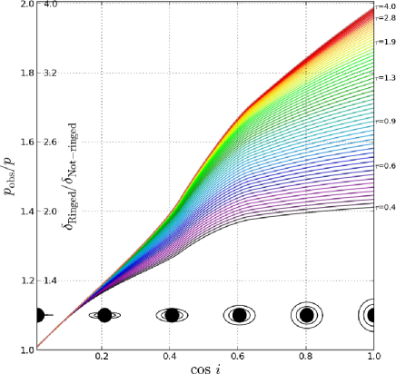
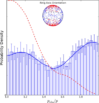
Figure 2.— Upper panel: ratio of observed to true planetary radius as a function of ring projected inclination ($\cos\,i$), assuming different values for the ring normal opacity ($\tau$). Lower panel: probability distribution of this ratio assuming completely random ring orientations (blue histogram) and a more concentrated distribution of planetary obliquities (red dashed line). For illustration purposes, we show, in the inset diagram, the distribution of random axis orientations used to compute both distributions. Each point represent the positions of the north and south pole of the planet for a given random orientation.

Ring transits could have a significant effect on the transit depth, $\delta$. To first order, $\delta$ provides the value of the apparent or observed planetary radius, $p_{\rm obs}$:

$$p_{\rm obs}=\sqrt{\delta}.$$ (8)

Thus, a significant overestimation of $\delta$ will also produce a substantial overestimation of the observed radius. In the absence of any other evidence for the presence of exorings, an anomalously deep transit may lead to the misclassification of a ringed planet as a false-positive or yield a gross underestimation of the planetary density.

To illustrate this, hereafter we assume the reference case of a planet with the same radius as Saturn $R_{\rm p}=0.0836R_{\odot}$ and rings of similar size and properties, i.e., $f_{\rm i}=1.58$ (inner edge of the A-ring) and $f_{\rm e}=2.35$ (outer edge of the B-ring). We assume for simplicity a value of $\tau=1$ (the opacity of B-ring ranges from 0.4-2.5, Murray & Dermott 1999). We also assume that the planet orbits a solar-mass star in a circular orbit at $a=1$ AU. The generalization of these results to other planetary, ring, and orbital parameters is trivial.

In Figure 2, we plot the ratio of observed to true planetary radius as obtained with Eqs. (1-3) for our reference planet.

In the extreme case of face-on rings, Eqs. (1-3) simplify to give

$$\lim_{i_{\rm R}\to 90^{\circ}}p_{\rm obs}=p\sqrt{1+(1-e^{-\tau})(f_{\rm e}^{2}-f_{\rm i}^{2})}.$$ (9)

The transits of a Saturn-like ringed planet are up to $\sim$3 times deeper than these expected for a spherical non-ringed one. These deep transits will be interpreted as being produced by a planet $\sim$1.7 times larger. Additionally, if independent estimations of its mass were also available, then the density of the planet would be underestimated by a factor of $\sim$5. Thus, instead of measuring Saturn’s density $\sim$0.7 g cm^-3, this planet would seem to have an anomalously low density of $\sim$0.14 g cm^-3. Even under more realistic orientations ($\cos i_{\rm R}\sim 0.2$), the observed radius will be $\sim$20% larger and the estimated density almost a half of the real one.

To assess the effect of rings on the observed planetary radius for an ensemble population of planets, we have calculated the probability distribution of the ratio $(p_{\rm obs}/p)$ assuming a uniform random ring orientation (obliquity and azimuthal angle, as defined in Ohta et al. 2009). The result is plotted in the lower panel of Figure 2 (blue histogram). The probability distribution corresponding to predominantly low obliquities (following a Fisher distribution in the case of a concentration parameter $\kappa\sim 8$ and 2-$\sigma$ obliquity dispersion of $\sim$ 30^∘) is also shown for comparison (red dashed line).

In the case of uniform random obliquities, more than 50% of the orientations lead to overestimations in planetary radius greater than $\sim$50%. This implies that with no other clues for the existence of rings around those planets, the bulk density of more than half of them would be underestimated by up to a factor of 3. With a more concentrated distribution of obliquities, the resulting radius distribution peaks at a null-effect of $(p_{\rm obs}/p)\sim 1$ but still exhibits considerable dispersion, with $\gtrsim$50% of the cases having observed radius anomalies $\gtrsim$ 30% (density overestimated by a factor $\gtrsim$2).

Deep transits are used as a criterion for flagging potential false-positives in photometric surveys (Batalha 2014; Burke et al. 2014). If a large unseen population of ringed planets exists, then we could have many potential candidates buried among misclassified false-positives. Therefore, we suggest that revisiting false-positive transits rejected with this criterion could potentially lead to the discovery of the first exoring population.

4. The Photo-ring effect (PR-EFFECT)

Under the simplified assumptions of the model presented in Section 2, an analytic solution for the orbital semimajor axis and impact parameter can be obtained from the basic transit parameters (Seager & Mallén-Ornelas 2003):

$$\left(\frac{a}{R_{\star}}\right)_{\rm obs} \approx \frac{P}{2\pi}\frac{\delta^{1/4}}{(T_{\rm 14}^{2}-T_{\rm 23}^{2})^{1/2}}$$ (10)

$$b_{\rm obs} \approx \left[\frac{T_{\rm 14}^{2}(1-\delta)-T_{\rm 23}^{2}(1+\delta)}{T_{\rm 14}^{2}-T_{\rm 23}^{2}}\right]^{1/2},$$ (11)

where we also assume $T_{\rm 14},T_{\rm 23}\ll P$, which is suitable for planets with $a\gg R_{\star}$, i.e., those worlds with improved chances for exorings.

Kepler’s third law relates the orbital period, semimajor axis, and stellar mass, such that we can calculate the mean stellar density:

$$\rho_{\rm\star,obs}=\frac{3\pi}{G}\frac{(a/R_{\star})_{\rm obs}^{3}}{P^{2}}$$ (12)

In the case of a transiting spherical planet, the observed value of $(a/R_{\star})_{\rm obs}$, and hence $\rho_{\rm\star,obs}$, are accurate estimates of their true values. If the planet, however, has a ring, then $\delta$, $T_{\rm 14}$ and $T_{\rm 23}$ will not be related by Equations (10) and (11), and the observed quantities will differ from the true ones.

A comparison of the observed density $\rho_{\rm\star,obs}$ with an independent measurement, $\rho_{\rm\star,true}$, such as that provided by stellar models, asteroseismology (Huber et al. 2013), or transits of other planetary companions, could indicate the existence of exorings.

In the upper panel of Figure 3, we show contours in the plane of the projected ring orientation of this so-called PR-effect.

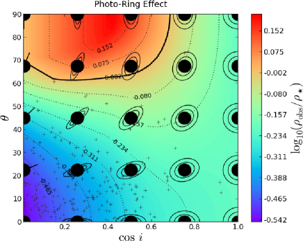
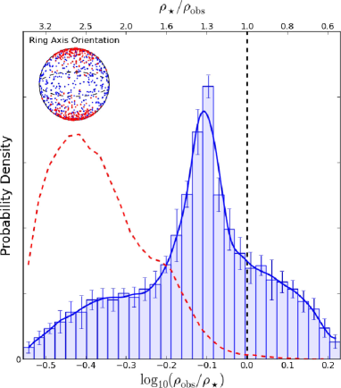
Figure 3.— Upper panel: contour plot of the PR effect. The crosses correspond to actual values of the projected inclinations for a subsample drawn from a low obliquity population (red dots in the inset plot of the lower panel). Lower panel: probability distribution of the PR effect for completely random orientations (blue) and for a more concentrated distribution of obliquities (red).

Since $T_{\rm 14}$ ($T_{\rm 23}$) is larger (smaller) when a ring is present (see Figure 1), the observed semimajor axis $a_{\rm obs}$ could be over- or underestimated. For large tilts ($\theta\sim 90^{\circ}$) and inclinations ($\cos i_{\rm R}\sim 0$), the transit duration will be the same as that of a non-ringed planet. Consequently, the increased transit depth $\delta$ will be the dominant effect in Eq. (10) and the observed density will be overestimated (upper left region in Figure 3).

For most values of the ring’s projected inclination and tilt, however, the transit duration will be modified to a larger extent than the depth, causing the semimajor axis and density to be underestimated. Therefore, rings tend to produce a negative PR effect (underestimation of stellar density) and this could be used to distinguish it from other asterodensity profiling (AP) effects discussed in Kipping (2014).

We can use Eqs. (4)-(7) to calculate an analytical expression for the maximum PR effect expected for a given external disk radius and impact parameter:

$$\left(\frac{\rho_{\rm\star,obs}}{\rho_{\rm\star,true}}\right)_{\rm max}\approx f_{\rm e}^{-3/2}(1-b^{2})^{-3/4}$$ (13)

For our reference case, $f_{\rm e}=2.35$, $b=0$, and the maximum value of the PR effect is $\log_{10}(\rho_{\rm\star,obs}/\rho_{\rm\star,true})\sim-0.6$. This corresponds to an underestimation of the stellar density by a noticeable factor of $\sim 4$.

We have calculated the probability distribution of the PR effect assuming similar priors to those used earlier. The results are shown in the lower panel of Figure 3.

In the uniform case, the ${\rm PR}$ distribution is strongly peaked around a negative value, $\log_{10}(\rho_{\rm\star,obs}/\rho_{\rm\star,true})\sim-0.2$. In contrast, if we consider obliquities no larger than $\sim$30^∘, then the peak shifts to $\log(\rho_{\rm\star,obs}/\rho_{\rm\star,true})\sim-0.45$, corresponding to a notable difference by a factor of $\sim$ 3 between the observed and true density.

The only other AP effects which can cause comparably large deviations are the photo-eccentric (PE) and the photo-blend effects, for which the former tends to cause a positive AP deviation and the latter a negative (Kipping 2014). In the case where blended companions can be excluded (e.g., through high-resolution imaging), then the ensemble distribution of the PR-effect should therefore be distinguishable from the other AP effects.

5. Discussion and Conclusions

In this Letter, we have presented a novel method for identifying exorings. Our method does not require a complex fit of transit light curves, instead relying on simple, analytic, and computationally efficient numerical procedures.

Our technique exploits the substantial impact that rings produce on the transit depth and duration, effects that can be independently confirmed by the measurement or estimation of other relevant astrophysical properties (e.g., stellar and planetary density).

Interestingly, the two effects we seek (anomalous transit depths and PR-effect) are complementary with respect to the orientation of the ring plane. For large inclinations and obliquities (face-on rings), the effect on transit depths is significant whilst the photo-ring effect is negligible. Alternatively, if rings have relatively low obliquities (egde-on rings), then the PR-effect will be considerable but the depth anomaly small.

Accordingly, three basic complementary strategies are proposed to identify exorings among the confirmed transiting exoplanets and candidates.

1. Search the confirmed transiting planets with anomalously low densities.

2. Search transiting objects that have been tagged as false positives due to anomalously large transit depths.

3. Search transit signals for which a negative AP effect is observed.

Besides aiding observers seeking interesting individual systems, the effects described here are well-suited for inferring a population of ringed planets. Ensemble studies using AP are in their infancy, but Sliski & Kipping (2014) recently conducted the first such analysis on a sample of 41 single Kepler planetary candidates with asteroseismically constrained host stars. In this limited sample, largely focused on short-period planets, the authors conclude that the 31 dwarf stars yield a broad AP distribution about zero, consistent with the expected photo-eccentric variations, whereas as the objects associated with giant stars are likely orbiting different stars altogether. A larger sample, including longer-period planets, would provide the opportunity to seek the expected offset due to the PR-effect too. This would require a reliable independent measure of the stellar density for stars too faint for asteroseismology, perhaps using methods such as “flicker” (Kipping et al. 2014a).

Low-density planets are also interesting targets when seeking exoplanetary rings. Over 10% of the already confirmed planets have estimated densities. Most of them are planets larger than Neptune, and a non-negligible fraction have anomalously low densities below $\sim$0.3 g cm^-3. Although several successful explanations have been devised for reconciling observed low densities with planetary interior and thermal evolutionary models (Miller et al. 2009), other anomalies still remain and may be worth a further analysis along the lines suggested here.

With the exception of Kepler-421b (Kipping et al. 2014b), all of the confirmed planets and most of Kepler candidates are inside the so-called snow line. Although icy rings, such as those observed around Saturn and Solar System giant planets, seem unlikely inside this limit, the existence of “warm” rocky rings at distances as short as $\sim$0.1 AU, are not dynamically excluded (Schlichting & Chang 2011).

We stress that the method presented here is complementary to the methods developed to discover exorings through detailed light curve modeling (Barnes & Fortney 2004; Ohta et al. 2009; Tusnski & Valio 2011). As explained earlier, the role of these methods will be very important once a suitable list of potential exoring candidates is created. It is, however, also important to note the great value of light curve models developed under the guiding principle of computational efficiency (semi-analytical formulae, efficient numerical procedures, etc), such as the basic models presented here.

Our simple technique is suitable for surveying entire catalogs of transiting planet candidates for exoring candidates, providing a subset of objects worthy of more detailed light curve analysis. Moreover, the technique is highly suited for uncovering evidence of a population of ringed planets by comparing the radius anomaly and PR-effects in ensemble studies. To aid the community, we provide the publicly available code at http://github.org/facom/exorings to simulate the novel effects described in this work.

Appendix A Area of the Ring

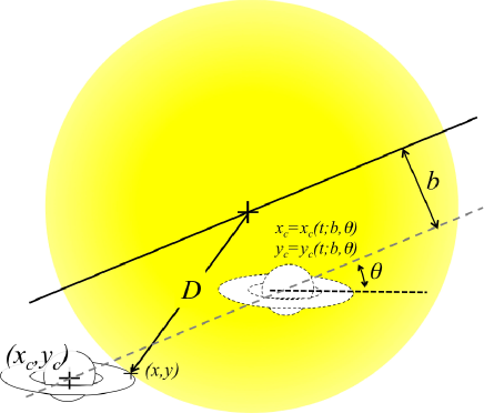
Figure 4.— Geometrical constructions used to compute ring area (left panel) and contact position (right panel). For contact position, a rotated reference system where the rings are horizontal considerably eases the analytic derivations.

The area obscured only by the ring is computed substracting the areas of the ellipse and circle sectors limited by interesection points E₁ and E₂ (Figure 4):

$$A_{\rm ring}=2(A_{\rm e}-A_{\rm c}).$$ (A1)

The area of the circle and ellipse sectors follow from the Cavallieri’s Principle:

$$A_{\rm c} = \frac{1}{2}\Delta\theta\;R^{2}$$ (A2)

$$A_{\rm e} = \frac{1}{2}\Delta E\;AB,$$

where $A$ and $B$ are the apparent semimajor and semiminor axes of the ring, $\Delta\theta$ is the angle subtended by the sector, and $\Delta E$ is the eccentric anomaly difference between E₁ and E₂.

The length of the segment joining E₁E₂ is:

$$\frac{s}{2}=B\sqrt{\frac{A^{2}-R^{2}}{A^{2}-B^{2}}}$$ (A3)

Simple trigonometrical relationships and the parametric equation of the ellipse provide us with the expressions for $\Delta\theta$ and $\Delta E$:

$$\Delta\theta = 2\arcsin\left(\frac{s}{2R}\right)$$ (A4)

$$\Delta E = 2\arcsin\left(\frac{s}{2B}\right).$$

Inserting Equations (A) into A, the areas are finally given by

$$A_{\rm c} = R^{2}\arcsin\left(\cos i_{\rm R}\frac{\sqrt{f^{2}-1}}{f\sin i_{\rm R}}\right)$$ (A5)

$$A_{\rm e} = f^{2}\cos i_{\rm R}\;R^{2}\arcsin\left(\frac{\sqrt{f^{2}-1}}{f\sin i_{\rm R}}\right).$$

From these areas and Eq. (A1), the effective ring radius in Eq. (3) follows trivially.

Appendix B Ring contact positions

Points over the external ring in the right panel of Figure 4 obey the following parametric equations:

$$x(E,t) = A\cos E+x_{c}(t)$$ (B1)

$$y(E,t) = B\sin E+y_{c}(t)$$

where $E$ is the eccentric anomaly, $x_{c}(t),y_{c}(t)$ are the instantaneous coordinates of the planet center, and $t$ is an arbitrary parameter (time for instance).

Contact positions are those for which the distance $D$ to origin,

$$D^{2}(E,t)=[A\cos E+x_{c}(t)]^{2}+[B\sin E+y_{c}(t)]^{2},$$ (B2)

obeys two conditions:

$$\left.\frac{\partial D^{2}}{\partial E}\right|_{E_{i},t_{i}} = 0$$ (B3)

$$D^{2}(E_{i},t_{i}) = R_{\star}^{2}$$

or explicitly:

$$A^{2}\cos^{2}E_{i}+B^{2}\sin^{2}E_{i}+x_{c}^{2}(t_{i})+y_{c}^{2}(t_{i})+2[A\,x_{c}(t)cosE_{i}+B\,y_{c}(t_{i})\sin E] = 0$$ (B4)

$$(B^{2}-A^{2})\sin E_{i}\cos E_{i}-A\,x_{c}(t_{i})\sin E+B\,y_{c}(t_{i})\cos E_{i}-R_{\star}^{2} = 0.$$

The solutions to these trigonometric equations, altough programmable, are not expressable in closed form.

The “empirical” formula in Eq. (5) was obtained after the approximations $A\gg B$ and $|\cos E_{i}|\sim 1$. This only works for $\cos i_{\rm R}\sim 0$ and $\theta\sim 0$. We have verified, however, that contact times estimated with Eq. (5), (6) and (7) are off by $\lesssim$1% in the case of contacts 3 and 4 for most ring projected orientations (provided $\theta>0$) and $\lesssim$10% for contacts 1 and 2. In the cases when $\theta\gtrsim 60^{\circ}$ or $\cos\,i\gtrsim 0.5$ a numerical solution for Eqs. (B4) is required to attain an acceptable precision.

References

- Barnes & Fortney (2004) Barnes, J. W., & Fortney, J. J. 2004, ApJ, 616, 1193
- Batalha (2014) Batalha, N. M. 2014, Proceedings of the National Academy of Science, 111, 12647
- Beichman et al. (2014) Beichman, C., Benneke, B., Knutson, H., et al. 2014, ArXiv e-prints, arXiv:1411.1754
- Burke et al. (2014) Burke, C. J., Bryson, S. T., Mullally, F., et al. 2014, ApJS, 210, 19
- Carter & Winn (2010) Carter, J. A., & Winn, J. N. 2010, ApJ, 716, 850
- Charbonneau et al. (2000) Charbonneau, D., Brown, T. M., Latham, D. W., & Mayor, M. 2000, ApJ, 529, L45
- Guyon et al. (2012) Guyon, O., Martinache, F., Cady, E. J., et al. 2012, in Society of Photo-Optical Instrumentation Engineers (SPIE) Conference Series, Vol. 8447, Society of Photo-Optical Instrumentation Engineers (SPIE) Conference Series, 1
- Heller et al. (2014) Heller, R., Williams, D., Kipping, D., et al. 2014, Astrobiology, 14, 798
- Henry et al. (2000) Henry, G. W., Marcy, G. W., Butler, R. P., & Vogt, S. S. 2000, ApJ, 529, L41
- Huber et al. (2013) Huber, D., Chaplin, W. J., Christensen-Dalsgaard, J., et al. 2013, ApJ, 767, 127
- Johns et al. (2012) Johns, M., McCarthy, P., Raybould, K., et al. 2012, in Society of Photo-Optical Instrumentation Engineers (SPIE) Conference Series, Vol. 8444, Society of Photo-Optical Instrumentation Engineers (SPIE) Conference Series, 1
- Kenworthy & Mamajek (2015) Kenworthy, M. A., & Mamajek, E. E. 2015, ApJ, 800, 126
- Kipping (2009) Kipping, D. M. 2009, MNRAS, 392, 181
- Kipping (2014) —. 2014, MNRAS, 440, 2164
- Kipping et al. (2014a) Kipping, D. M., Torres, G., Buchhave, L. A., et al. 2014a, ApJ, 795, 25
- Kipping et al. (2014b) —. 2014b, ApJ, 795, 25
- Leconte et al. (2011) Leconte, J., Lai, D., & Chabrier, G. 2011, A&A, 528, A41
- Mamajek et al. (2012) Mamajek, E. E., Quillen, A. C., Pecaut, M. J., et al. 2012, AJ, 143, 72
- Miller et al. (2009) Miller, N., Fortney, J. J., & Jackson, B. 2009, ApJ, 702, 1413
- Murray & Dermott (1999) Murray, C. D., & Dermott, S. F. 1999, Solar system dynamics. Cambridge University Press.
- Ohta et al. (2009) Ohta, Y., Taruya, A., & Suto, Y. 2009, ApJ, 690, 1
- Rauer & Catala (2011) Rauer, H., & Catala, C. 2011, in IAU Symposium, Vol. 276, IAU Symposium, ed. A. Sozzetti, M. G. Lattanzi, & A. P. Boss, 354–358
- Ricker et al. (2014) Ricker, G. R., Winn, J. N., Vanderspek, R., et al. 2014, in Society of Photo-Optical Instrumentation Engineers (SPIE) Conference Series, Vol. 9143, Society of Photo-Optical Instrumentation Engineers (SPIE) Conference Series, 20
- Sackett (1999) Sackett, P. D. 1999, in NATO Advanced Science Institutes (ASI) Series C, Vol. 532, NATO Advanced Science Institutes (ASI) Series C, ed. J.-M. Mariotti & D. Alloin, 189
- Schlichting & Chang (2011) Schlichting, H. E., & Chang, P. 2011, ApJ, 734, 117
- Seager & Mallén-Ornelas (2003) Seager, S., & Mallén-Ornelas, G. 2003, ApJ, 585, 1038
- Sliski & Kipping (2014) Sliski, D. H., & Kipping, D. M. 2014, ApJ, 788, 148
- Tusnski & Valio (2011) Tusnski, L. R. M., & Valio, A. 2011, ApJ, 743, 97
- Vidotto et al. (2010) Vidotto, A. A., Jardine, M., & Helling, C. 2010, ApJ, 722, L168