22email: djelloul.ziadi@univ-rouen.fr
Efficient Geometric-based Computation of the String Subsequence Kernel††thanks: This work is supported by the MESRS - Algeria under Project 8/U03/7015.
Abstract
Kernel methods are powerful tools in machine learning. They have to be computationally efficient. In this paper, we present a novel Geometric-based approach to compute efficiently the string subsequence kernel (SSK). Our main idea is that the SSK computation reduces to range query problem. We started by the construction of a match list where and are the strings to be compared; such match list contains only the required data that contribute to the result. To compute efficiently the SSK, we extended the layered range tree data structure to a layered range sum tree, a range-aggregation data structure. The whole process takes time and space, where is the size of the match list and is the length of the SSK. We present empiric evaluations of our approach against the dynamic and the sparse programming approaches both on synthetically generated data and on newswire article data. Such experiments show the efficiency of our approach for large alphabet size except for very short strings. Moreover, compared to the sparse dynamic approach, the proposed approach outperforms absolutely for long strings.
Keywords:
string subsequence kernel, computational geometry, layered range tree, range query, range sum1 Introduction
Kernel methods [4] offer an alternative solution to the limitation of traditional machine learning algorithms, applied solely on linear separable problems. They map data into a high dimensional feature space where we can apply linear learning machines based on algebra, geometry and statistics. Hence, we may discover non-linear relations. Moreover, kernel methods enable other data type processings (biosequences, images, graphs, …).
Strings are among the important data types. Therefore, machine learning community devotes a great effort of research to string kernels, which are widely used in the fields of bioinformatics and natural language processing. The philosophy of all string kernels can be reduced to different ways to count common substrings or subsequences that occur in both strings to be compared, say and .
In the literature, there are two main approaches to improve the computation of the SSK. The first one is based on dynamic programming; Lodhi et al. [6] apply dynamic programming paradigm to the suffix version of the SSK. They achieve a complexity of , where is the length of the SSK. Later, Rousu and Shawe-Taylor [7] propose an improvement to the dynamic programming approach based on the observation that most entries of the dynamic programming matrix (DP) do not really contribute to the result. They use a set of match lists combined with a sum range tree. They achieve a complexity of , where is the set of matches of characters in the two strings. Beyond the dynamic programming paradigm, the trie-based approach [5, 7, 8] is based on depth first traversal on an implicit trie data structure. The idea is that each node in the trie corresponds to a co-occurrence between strings. But the number of gaps is restricted, so the computation is approximate.
Motivated by the efficiency of the computation, a key property of kernel methods, in this paper we focus on improving the SSK computation. Our main idea consists to map a machine learning problem on a computational geometry one. Precisely, our geometric-based SSK computation reduces to 2-dimensional range queries on a layered range sum tree (a layered range tree that we have extended to a range-aggregate data structure). We started by the construction of a match list where and are the strings to be compared; such match list contains only the required data that contribute to the result. To compute efficiently the SSK, we constructed a layered range sum tree and applied the corresponding computational geometry algorithms. The overall time complexity is , where is the size of the match list.
The rest of this paper is organized as follows. Section 2 deals with some concept definitions and introduces the layered range tree data structure. In section 3, we recall formally the SSK computation. We also review three efficient computations of the SSK, namely, dynamic programming, trie-based and sparse dynamic programming approaches. Our contribution is addressed in Section 4. Section 5 presents the conducted experiments and discusses the associated results, demonstrating the practicality of our approach for large alphabet sizes. Section 6 presents conclusions and further work.
2 Preliminaries
We first deal with concepts of string, substring, subsequence and kernel. We then present the layered range tree data structure.
2.1 String
Let be an alphabet of a finite set of symbols. We denote the number of symbols in by . A string is a finite sequence of symbols of length where marks the element of . The symbol denotes the empty string. We use to denote the set of all finite strings of length and the set of all strings. The notation is a boolean function that returns
2.2 Substring
For , the string denotes the substring of . Accordingly, a string is a substring of a string if there are strings and such that ( and can be empty). The substrings of length are referred to as -grams (or -mers).
2.3 Subsequence
The string is a subsequence of if there exists an increasing sequence of indices in , such that , for . In the literature, we use if is a subsequence of in the positions given by . The empty string is indexed by the empty tuple. The absolute value denotes the length of the subsequence which is the number of indices , while refers to the number of characters of covered by the subsequence .
2.4 Kernel methods
Traditional machine learning and statistic algorithms have been focused on linearly separable problems (i.e. detecting linear relations between data). It is the case where data can be represented by a single row of table. However, real world data analysis requires non linear methods. In this case, the target concept cannot be expressed as simple linear combinations of the given attributes [4]. This was highlighted in 1960 by Minsky and Papert.
Kernel methods were proposed as a solution by embedding the data in a high dimensional feature space where linear learning machines based on algebra, geometry and statistics can be applied. This embedding is called kernel. It arises as a similarity measure (inner product) in a high dimension space so-called feature description.
The trick is to be able to compute this inner product directly from the original data space using the kernel function. This can be formally clarified as follows: the kernel function corresponds to the inner product in a feature space via a map .
2.5 Layered Range Tree
A Layered Range Tree (LRT) is a spatial data structure that supports orthogonal range queries. It is judicious to describe a 2-dimensional range tree inorder to understand LRT. Consider a set of points in . A range tree is primarily a balanced binary search tree (BBST) built on the -coordinate of the points of . Data are stored in the leaves only. Every node in the BBST is augmented by an associated data structure () whitch is a 1-dimensional range tree, it can be a BBST or a sorted array, of a canonical subset on -coordinates. The subset is the points stored in the leaves of the sub tree rooted at the node . Figure 1 depicts a 2-dimensional range tree for a set of points . In the case where two points have the same or -coordinate, we have to define a total order by using a lexicographic one. It consists to replace the real number by a composite-number space [2]. The composite number of two reals and is denoted by , so for two points, we have:
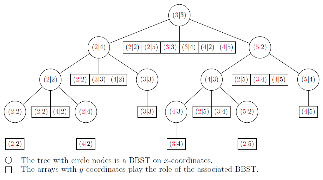
Based on the analysis of computational geometry algorithms, our 2-dimensional range tree for a set of points requires storage and can be constructed in time.
The range search problem consists to find all the points of that satisfy a range query. A useful idea, in terms of efficiency, consists on treating a rectangular range query as a two nested 1-dimensional queries. In other words, let be a 2-dimensional range query, we first ask for the points with -coordinates in the given 1-dimensional range query . Consequently, we select a collection of subtrees. We consider only the canonical subset of the resulted subtrees, which contains, exactly, the points that lies in the -range .
At the next step, we will only consider the points that fall in the -range .
The total task of a range query can be performed in time, where is the number of points that are in the range. We can improve it by enhancing the 2-dimensional range tree with the fractional cascading technique which is described in the following paragraph.
The key observation made during the invocation of a rectangular range query is that we have to search the same range in the associated structures of nodes found while querying the main BBST by the range query . Moreover, there exists an inclusion relationship between these associated structures. The goal of the fractional cascading consists on executing the binary search only once and use the result to speed up other searches without expanding the storage by more than a constant factor.
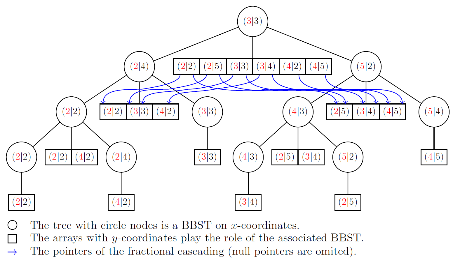
The application of the fractional cascading technique introduced by [3] on a range tree creates a new data structure so called layered range tree. The technique consists to add pointers from the entries of an associated data structure of some level to the entries of an associated data structure below, say as follows: If stores a value with the key , then we store a pointer to the entry in with the smallest key larger than or equal . We illustrate such technique in Fig. 2 for the same set represented in Fig. 1. Using this technique, the rectangular search query time becomes , for the first binary search and for browsing the reported points.
3 String Subsequence Kernels
The philosophy of all string kernel approaches can be reduced to different ways to count common substrings or subsequences that occur in the two strings to compare. This philosophy is manifested in two steps:
-
•
Project the strings over an alphabet to a high dimension vector space , where the coordinates are indexed by a subset of the input space.
-
•
Compute the distance (inner product) between strings in . Such distance reflects their similarity.
For the String Subsequence Kernel (SSK) [6], the main idea is to compare strings depending on common subsequences they contain. Hence, the more similar strings are ones that have the more common subsequences. However, a new weighting method is adopted. It reflects the degree of contiguity of the subsequence in the string. In order to measure the distance of non contiguous elements of the subsequence, a gap penalty is introduced. Formally, the mapping function in the feature space can be defined as follows:
The associated kernel can be written as:
In order to clarify the idea of the SSK, we present a widespread example in the literature. Consider the strings , , and , for a subsequence length , the mapping to the feature space is as follows:
| ar | at | ba | br | bt | ca | cr | ct | |
|---|---|---|---|---|---|---|---|---|
| bar | 0 | 0 | 0 | 0 | 0 | |||
| bat | 0 | 0 | 0 | 0 | 0 | |||
| car | 0 | 0 | 0 | 0 | 0 | |||
| cat | 0 | 0 | 0 | 0 | 0 |
The unnormalized kernel between and is , while the normalized version is obtained by :
A direct implementation of this kernel leads to time and space complexity. Since this is the dimension of the feature space. To assist the computation of the SSK a Suffix Kernel is defined through the embedding given by:
where denotes the set of -tuples of indices with . In other words, we consider only the subsequences of length that the last symbol is identical to the last one of the string . The associated kernel can be defined as follows:
To illustrate this kernel counting trick, we take back the precedent example where the mapping is as follows:
| ar | at | ba | br | bt | ca | cr | ct | |
|---|---|---|---|---|---|---|---|---|
| bar | 0 | 0 | 0 | 0 | 0 | 0 | ||
| bat | 0 | 0 | 0 | 0 | 0 | 0 | ||
| car | 0 | 0 | 0 | 0 | 0 | 0 | ||
| cat | 0 | 0 | 0 | 0 | 0 | 0 |
for example
and
The SSK can be expressed in terms of its suffix version as:
| (1) |
with
3.1 Naive Implementation
The computation of the similarity of two strings ( and ) is conditioned by their final symbols. In the case where , we have to sum kernels of all prefixes of and . Hence, a recursion has to be devised:
| (2) |
This computation leads to a complexity of .
3.2 Efficient Implementations
We present three methods that compute the SSK efficiently, namely the dynamic programming [6], the trie-based [5, 7, 8] and the sparse dynamic programming approaches [7].
To describe such approaches, we use two strings and as a running example.
3.2.1 Dynamic Programming Approach.
The starting point of the dynamic programming approach is the suffix recursion given by equation (2). From this equation, we can consider a separate dynamic programming table for storing the double sum:
| (3) |
It is easy to see that: .
Computing ordinary for each would be inefficient. So we can devise a recursive version of equation (3) with a simple counting device:
Consequently, using the dynamic programming approach (Algorithm 1), the complexity of the SSK becomes .
Table 1 illustrates the computation of the dynamic programming tables for the running example for . The evaluation of the kernel is given by the sum of entries of the suffix table KPS:
| g | a | t | t | a | |
| c | |||||
| a | |||||
| t | |||||
| a | |||||
| g | a | t | t | a | |
| c | 0 | 0 | 0 | 0 | |
| a | 0 | ||||
| t | 0 | ||||
| a | |||||
| g | a | t | t | a | |
| c | |||||
| a | |||||
| t | |||||
| a |
3.2.2 Trie-based Approach.
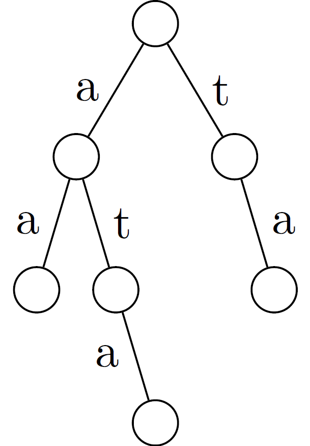
This approach is based on search trees known as tries, introduced by E. Fredkin in 1960. The key idea of the trie-based approach is that leaves play the role of the feature space indexed by the set of strings of length . In the literature, there are variants of trie-based string subsequence kernels. For instance the -mismatch string kernel [5] and restricted SSK [8].
| 0 | ||||||
| 1 | ||||||
| 2 | ||||||
| 3 | ||||||
| 0 | ||||||
| 1 | ||||||
| 2 | ||||||
| 3 |
In the present section, we try to describe a trie-based SSK presented in [7] that slightly differ from those cited above [5, 8]. Figure 3 illustrates the trie data structure for the running example. Each node in the trie corresponds to a co-occurrence between strings. The algorithm maintains for all matches , a list of alive matches as presented in Table 2 that records the last index where is the number of gaps in the match. Notice that in the same list we are able to record many occurrences with different gaps. Alive lists for longer matches , can be constructed incrementally by extending the alive list corresponding to . Similarly, the algorithm is applied to the string . The process will continue until achieving the depth . For efficiency reasons, we need to restrict the number of gaps to a given integer , so the computation is approximate. The kernel is evaluated as follows:
Given that, there are possible combinations to assign letters and gaps in a window of length , the worst-case time complexity of the algorithm is .
The string subsequence kernel for the running example for is:
Similar computation is performed for and :
and
3.2.3 Sparse Dynamic Programming Approach.
It is built on the fact that in many cases, most of the entries of the matrix are zero and do not contribute to the result. Rousu and Shawe-Taylor [7] have proposed a solution using the sparse dynamic programming technique to avoid unnecessary computations. To do so, two data structures were proposed: the first one is a range sum tree, which is a B-tree, that replaces the matrix. It is used to return the sum of values within an interval in time. The second one is a set of match lists instead of matrix. where . This dummy gap weight allows to address the problem of scaling the kernel values as the computation progress. Consequently the recursion (2) becomes:
| (4) |
and the separate dynamic programming table (3) can be expressed as follows:
| (5) |
Thereafter, the authors devise a recursive version of (5):
| (6) |
This can be interpreted as reducing the evaluation of an orthogonal range query (5) to an evaluation of a simple range query multiple times as much as the number of lines of the matrix.
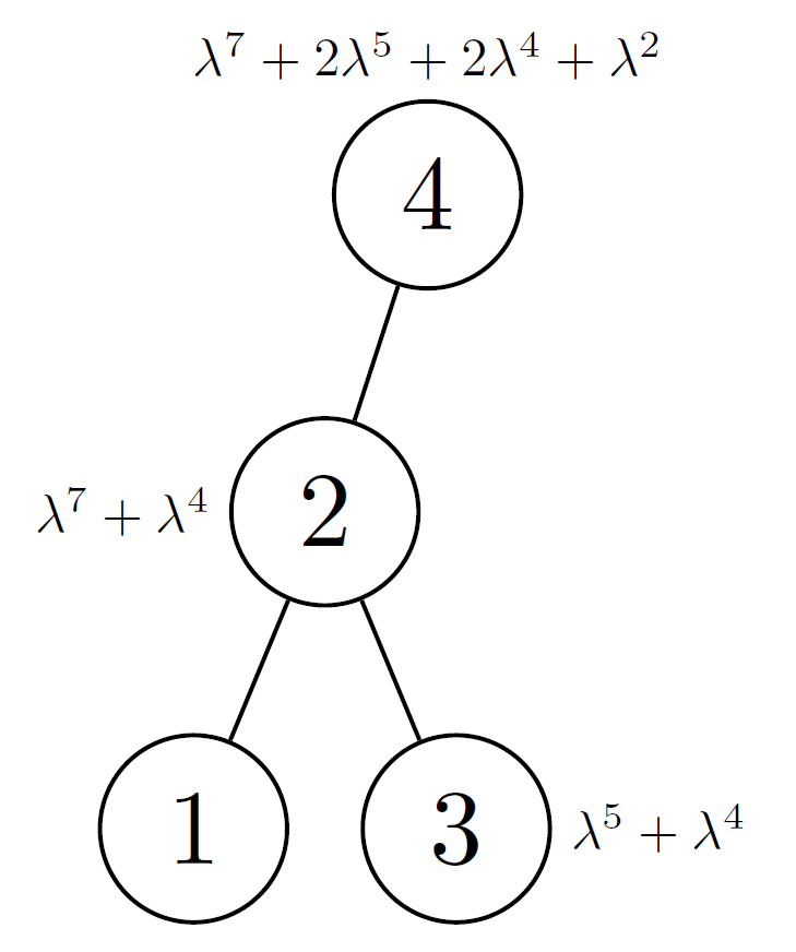
To evaluate efficiently a range query, the authors use a range-sum tree to store a set of key-value pairs. A range-sum tree is a binary tree of height where each node in depth contains a key with a sum of values in a sub range . The root is labeled with , the left child of a node is and the right child if it exists is . Odd keys label the leaves of the tree.
To compute the range sum of values within an interval it suffices to browse the path from the node j to the root and sum over the left subtrees as follows:
Moreover to update the value of a node , we need to update all the values of parents that contain in their subtree (). These two operations are performed in time because we traverse in the worst case the height of the tree.
For the sparse dynamic programming algorithm (Algorithm 2) the range-sum tree is used incrementally when computing (6). So that when processing the match list the tree will contain the values that satisfy . Hence the evaluation of (6) is performed by involving a one dimensional range query:
Concerning the cost of computation of this approach, the set of match lists is created on time and space, while the kernel computation time is , knowing that .
To illustrate the mechanism of the sparse dynamic programming algorithm, Figure 4 depicts the state of the range-sum tree when computing .
Initially the set of match lists is created as follows:
Meanwhile maintaining the range-sum tree, the algorithm update the set of match lists as presented below:
Finally, summing the values of the updated match list after discarding the dummy weight gives the kernel value :
4 Geometric based Approach
Looking forward to improving the complexity of SSK, our approach is based on two observations. The first one concerns the computation of that is required only when . Hence, we have kept only a list of index pairs of these entries rather than the entire suffix table,
In the rest of the paper, while measuring the complexity of different computations, we will consider, , the size of the match list as the parameter indicating the size of the input data.
The complexity of the naive implementation of the list version is , and it seems not obvious to compute efficiently on a list data structure. In order to address this problem, we have made a second observation that the suffix table can be represented as a 2-dimensional space (plane) and the entries where as points in this plane as depicted in Fig. 5. In this case, the match list generated is
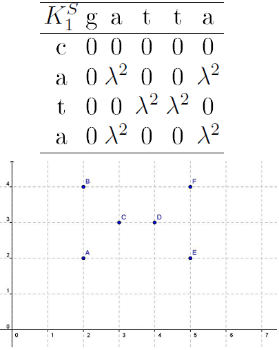
With a view to improving the computation of the SSK, it is easy to perceive from Fig. 5 that the computation of (2) can be interpreted as orthogonal range queries. In this respect, we have used a layered range tree (LRT) in [1]. But the LRT data structure reports all points that lie in a specific range query. However, for the SSK computation we require only the sum of values of the reported points.
To achieve this goal, we extend the LRT with the aggregate operations, in particular the summation one. Hence, a novel data structure was created, for instance a Layered Range Sum Tree (LRST). A LRST is a LRT with two substantial extensions to reduce the range sum query time from to where is the number of reported points in the range.
The first extension consists to substitute the associated data structures in the LRT with new associated data structures where each entry contains a key-value pair , is the partial sum of in the position . This extension is made to compute the range sum of within in time as follows : .
The second extension involves the fractional cascading technique. Let and be two sorted arrays that store partial sums of and respectively. Suppose that we want to compute the range sum within a query in and . We start with a binary search with in to find the smallest key larger than or equal . We make also an other binary search with in to find the largest key smaller than or equal . If an entry stores a key then we store a pointer to the entry in with the smallest key larger than or equal to , say small pointer, and a second pointer to the entry in with the largest key smaller than or equal to , say large pointer. If there is no such key(s) then the pointer(s) is (are) set to nil.
It is easy to see that our extensions does not affect neither the space nor the time complexities of the LRT construction. So according to the analysis of of computational geometry algorithms, our LRST requires storage and can be constructed in time. This leads to the following lemma.
Lemma 1
Let and be two strings and the match list associated to the suffix version of the SSK. A Layered range sum tree (LRST) for requires storage and takes construction time.
We can now exploit these extensions to compute efficiently the range sum inherent to in and . Let and be the results of the binary search with and respectively in . So the in takes time. To compute the range sum in we avoid the binary searches. We consider first the entry pointed by the small pointer of , it contains the smallest key from larger than or equal to . The second entry is pointed by the large pointer of , it contains the largest key from smaller than or equal to . Finally the range sum within in is given by and it takes time.
For our geometric approach (Algorithm 3) we will use the LRST to evaluate the SSK. We start by the creation of the match list where . This trick is inspired from [7] to make the range sum results correct. Thus the recursion (2) becomes as follows:
| (7) |
In order to construct efficiently the match list we have to create for each character a list of occurrence positions in the string . Thereafter, for each character we insert key-value pairs in the match list corresponding to . This process takes space and time. For example, the match list for our running example is .
Once the initial match list created, we start computing the SSK for the subsequence length . This computation doesn’t require the LRST ; it suffices to traverse the match list and sum over its values. For length subsequence we will first create the LRST corresponding to the match list, afterward for each item we invoke the LRST with the query . This latter return the range sum within : . If is positive then insert the key-value in a new match list for the level and summing the to compute the SSK at the level . At each iteration, we have to create a new LRST corresponding to the new match list until achieving the request subsequence length .
We recall that in our case, we use composite numbers instead of real numbers, see section (2.5). In such situation, we have to transform the range query related to a set of points in the plane to the range query related to the composite space.
Using our geometric approach, the range sum query time becomes . For the computation of we have to consider entries of the match list. The process iterates times, therefore, we get a time complexity of for evaluating the SSK. This result combined to that of Lemma. 1 lead to the following theorem that summarizes the result of our proposed approach to compute SSK.
Theorem 4.1
Let and be two strings and the match list associated to the suffix version of the SSK. A layered range sum tree requires storage and it can be constructed in time. With these data structures, the SSK of length can be computed in ).
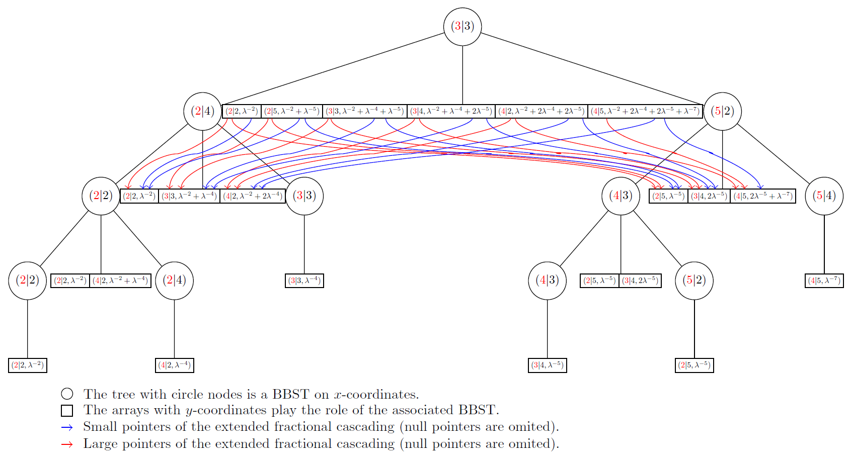
To compute , for our running example, we have to invoke the range sum on the LRST at the step represented by Fig.6. The SSK computation is performed by summing over all the range sums correponding th the entries of the match list as follows: .
To describe how this can be processed, we deal by the range sum of the query . At the associate data structure corresponding to the split node of Fig.6 we find the entries and whose are the smallest one larger than or equal to and the largest one smaller or equal to respectively. This can be done by binary search. Next, we look for the nodes that are below the split node and that are the right child of a node on the search path to where the path go left, or the left child of a node on the search path to where the path go right. The collected nodes are and the result returned form the associated data structures is . This is done on a constant time by following the small and large pointers form the associated data structure of the split node. By the same process we obtain the following results of the invoked range sums:
After rescaling the returned values by the factor we obtain the value of .
While invoking the range sums we will prepare the new match list for the next step. In our case the new match list contains the following matchs : .
5 Experimentation
In this section we describe the experiments that focus on the evaluation of our geometric algorithm against the dynamic and the sparse dynamic ones. Thereafter, these algorithms are referenced as Geometric, Dynamic and Sparse respectively. We have discarded the trie-based algorithm from this comparison because it is an approximate algorithm on the one hand, on the other hand in the preliminary experiments conducted in [7] it was significantly slower than Dynamic and Sparse.
To benefit from the empiric evaluation conducted in [7], we tried to keep the same conditions of their experiments. For this reason, we have conducted a series of experiments on both synthetically generated and on newswire article data on Reuter’s news articles.
We ran the tests on Intel Core i7 at 2.40 GHZ processor with 16 GB RAM under Windows 8.1 64 bit. We implemented all the tested algorithms in Java. For the LRST implementation, we have extended the LRT implementation available on the page https://github.com/epsilony/.
5.1 Experiments with synthetic data
These experiments concern the effects of the string length and the alphabet size on the efficiency of the different approaches and to determine under which conditions our approach outperforms.
We randomly generated string pairs with different lengths over alphabets of different sizes . To simplify the string generation, we considered string symbols as integer in . For convenience of data visualization, we have used the logarithmic scale on all axes. To perform accurate experiments, we have generated multiple pairs for the same string length and alphabet size and for each pair we have took multiple measures of the running time with a subsequence length and a decay parameter .
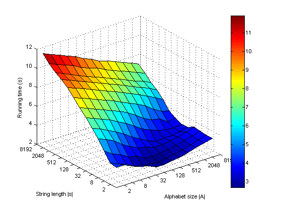
This being said, Fig. 7 reveals, for our geometric approach, an inverse dependency of the running time with the alphabet size. However, for an alphabet size the running time is proportional to the string length.
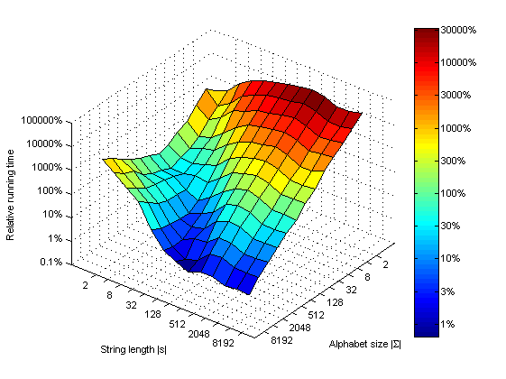
Figure 8 shows experimental comparison of the performance of the proposed approach against Dynamic. Note that the rate of indicates that the two algorithms deliver the same performances. For the rates less than our approach outperforms, it is the case for strings based on medium and large alphabets excepting those having short length (say alphabet size great than or equal , where the string length exceeds characters). For short strings and also for long strings based on small alphabets, Dynamic excels.
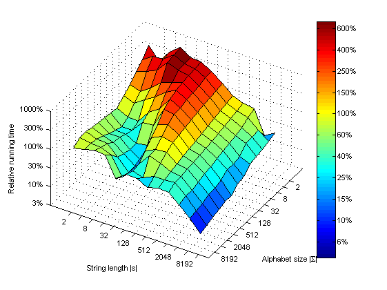
It remains to present results of the comparison experiment with Sparse which share the same motivations with our approach. Rousu and Shawe-Taylor [7] state that with long strings based on large alphabets their approach is faster. Figure 9 shows that in these conditions our approach dominates. Moreover, our approach is faster than the Sparse one for long strings and for large alphabets absolutely, but gets slower than Sparse for short strings based on small alphabets.
5.2 Experiments with newswire article data
Our second experiments use the Reuters-21578 collection to evaluate the speed of Geometric against Dynamic and Sparse on English articles. We created a dataset represented as sequences of syllables by transferring all the XML articles on to text documents. Thereafter, the text documents are preprocessed by removing stop words, punctuation marks, special symbols and finally word syllabifying. We have generated distinct syllables. As in the first experiment, each syllable alphabet is assigned an integer. To treat the documents randomly, we have shuffled this preliminary dataset.
For visualization convenience, while creating document pairs, we have ensured that their lengths are close. Under this condition, we have collected pair documents as final dataset.
To compare the candidate algorithms, we have computed the SSK for each document pair of the data set by varing the subsequence length form to . Figure 10 and Figure 11 depict the clusters of documents where Geometric is faster than Dynamic and Sparse respectively. A document pair is plotted according to the inverse match frequency (X-axis) and the document size (Y-axis). The inverse match frequency is given by: , it plays the role of the alphabet size inherent to the documents and . The document size is calculated as the arithmetic mean of the document pair sizes, it plays the role of the string length. Each cluster is distinguished by a special marker that corresponds to the necessary minimum subsequence length to make Geometric faster than Dynamic or Sparse. For the cluster marked by black diamonds, is sufficient. The length is required for the cluster marked by blue filled squares. For the cluster marked by green circles is required and the last cluster marked by plus signs is needed.
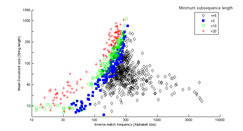
We can distinguish three cases in Fig. 10. The first one arises when the inverse match frequency is weak (small alphabet size), that is to say for dense matrix. In this case, we require important values of the subsequence length ( for small documents and for larger ones) to make Geometric faster than Dynamic. The second case concerns good inverse match frequencies (large alphabet size) corresponding to sparse matrix. In this case, small values of the subsequence length () suffice to make Geometric faster than Dynamic. The third case appear for moderate inverse match frequency (medium alphabet size), the values of that makes Geometric faster than Dynamic depend on the document size. The large document size the large is required.
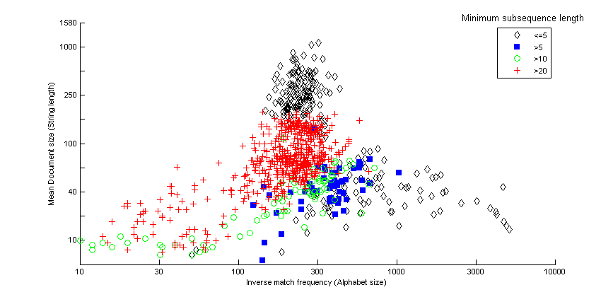
The results of the comparison between Geometric and Sparse on newswire article data are depicted in Fig. 11. We can discuss 3 cases: The first case emerge when the document size becomes large and also for good inverse match frequency. In this case small values of the subsequence length () suffice to make Geometric faster than Sparse. The second case appear for small documents and bad inverse match frequencies. The necessary subsequence length must be important ( for very small documents and for the small ones). The third case concerns modurate inverse frequencies. In this case the value of the subsequence length that makes Geometric faster than Sparse depends on the document size except large sizes which fall in the first case.
5.3 Discussion of the experiment results
In step with the results of the two experiments, it is easy to see that the algorithms behave essentially in the same way both on synthetically generated data and newswire article data. These results reveal that our approach outperforms for large alphabet size except for very small strings. Moreover, regarding to the Sparse, Geometric is competitive for long strings.
We can argue this as follows: first, the alphabet size and the string length affect substantially the kernel matrix form. Large alphabets can reduce potentially the partially matching subsequences especially on long strings, giving rise to sparse matrix form. Consequently, great number of data stored in the kernel matrix do not contribute to the result. In the other cases, for dense matrix, our approach can be worse than Dynamic by at most factor.
On the other hand, The complexities of Geometric and Sparse differ only by the factors and . The inverse dependency of and goes in favor of our approach. Also, the comparisons conducted on our datasets give evidence that for long strings , remembering that the size of the match list decrease while the SSK execution progress. Moreover, to answer orthogonal range queries, Sparse invoke one dimensional range query multiple times. Whereas, Geometric mark good scores by using orthogonal range queries in conjunction with the fractional cascading and exploit our extension of the LRT data structure to get directly the sum within a range.
6 Conclusions and further work
We have presented a novel algorithm that efficiently computes the string subsequence kernel (SSK). Our approach is refined over two phases. We started by the construction of a match list that contains, only, the information that contributes in the result. Thereafter, in order to compute, efficiently, the sum within a range for each entry of the match list, we have extended a layered range tree to be a layered range sum tree. The Whole task takes time and space, where is the length of the SSK and is the initial size of the match list.
The reached result gives evidence of an asymptotic complexity improvement compared to that of a naive implementation of the list version . The experiments conducted both on synthetic data and newswire article data attest that the dynamic programming approach is faster when the kernel matrix is dense. This case is achieved on long strings based on small alphabets and on short strings. Furthermore, recall that our approach and the sparse dynamic programming one are proposed in the context where the most of the entries of the kernel matrix are zero, i.e. for large-sized alphabets. In such case our approach outperforms. For long strings our approach behave better than the sparse one.
This well scaling of the proposed approach with document size and alphabet size could be useful in very tasks of machine learning on long documents as full-length research articles.
A noteworthy advantage is that our approach can be favorable if we assume that the problem is multi-dimensional. In terms of complexity, this can have influence the storage and the running time, only, by a logarithmic factor. Indeed, the layered range sum tree needs storage and can compute the sum within a rectangular range in , in a -dimensional space.
At the implementation level, great programming effort is supported by well-studied and ready to use computational geometry algorithms. Hence, the emphasis is shifted to a variant of string kernel computations that can be easily adapted.
Finally, it would be very interesting if the LRST can be extended to be a dynamic data structure. This can relieve us to create a new LRST at each evolution of the subsequence length. An other interesting axis consists to combine the LRST with the dynamic programming paradigm. We believe that using rectangular intersection techniques seems to be a good track, though this seems to be a non trivial task.
References
- [1] Bellaouar, S., Cherroun, H., Ziadi, D.: Efficient list-based computation of the string subsequence kernel. In: LATA’14. pp. 138–148 (2014)
- [2] Berg, M.d., Cheong, O., Kreveld, M.v., Overmars, M.: Computational Geometry: Algorithms and Applications. Springer-Verlag TELOS, Santa Clara, CA, USA, 3rd ed. edn. (2008)
- [3] Chazelle, B., Guibas, L.J.: Fractional cascading: I. a data structuring technique. Algorithmica 1(2), 133–162 (1986)
- [4] Cristianini, N., Shawe-Taylor, J.: An introduction to support Vector Machines: and other kernel-based learning methods. Cambridge University Press, New York, NY, USA (2000)
- [5] Leslie, C., Eskin, E., Noble, W.: Mismatch String Kernels for SVM Protein Classification. In: Neural Information Processing Systems 15. pp. 1441–1448 (2003), http://citeseerx.ist.psu.edu/viewdoc/summary?doi=10.1.1.58.4737
- [6] Lodhi, H., Saunders, C., Shawe-Taylor, J., Cristianini, N., Watkins, C.: Text classification using string kernels. J. Mach. Learn. Res. 2, 419–444 (Mar 2002), http://dx.doi.org/10.1162/153244302760200687
- [7] Rousu, J., Shawe-Taylor, J.: Efficient computation of gapped substring kernels on large alphabets. J. Mach. Learn. Res. 6, 1323–1344 (Dec 2005), http://dl.acm.org/citation.cfm?id=1046920.1088717
- [8] Shawe-Taylor, J., Cristianini, N.: Kernel Methods for Pattern Analysis. Cambridge University Press, New York, NY, USA (2004)