sCOLA: The N-body COLA Method Extended to the Spatial Domain
Abstract
We present sCOLA – an extension of the N-body COmoving Lagrangian Acceleration (COLA) method to the spatial domain. Similar to the original temporal-domain COLA, sCOLA is an N-body method for solving for large-scale structure in a frame that is comoving with observers following trajectories calculated in Lagrangian Perturbation Theory. Incorporating the sCOLA method in an N-body code allows one to gain computational speed by capturing the gravitational potential from the far field using perturbative techniques, while letting the N-body code solve only for the near field. The far and near fields are completely decoupled, effectively localizing gravity for the N-body side of the code. Thus, running an N-body code for a small simulation volume using sCOLA can reproduce the results of a standard N-body run for the same small volume embedded inside a much larger simulation. We demonstrate that sCOLA can be safely combined with the original temporal-domain COLA. sCOLA can be used as a method for performing zoom-in simulations. It also allows N-body codes to be made embarrassingly parallel, thus allowing for efficiently tiling a volume of interest using grid computing. Moreover, sCOLA can be useful for cheaply generating large ensembles of accurate mock halo catalogs required to study galaxy clustering. Surveys that will benefit the most are ones with large aspect ratios, such as pencil-beam surveys, where sCOLA can easily capture the effects of large-scale transverse modes without the need to substantially increase the simulated volume. As an illustration of the method, we present proof-of-concept zoom-in simulations using a freely available sCOLA-based N-body code.
1 Introduction
Understanding Large Scale Structure (LSS) of the universe has been a multi-generational effort in understanding the macroscopic physics governing the evolution of the universe, arising from a trivial microscopic law – the law of universal gravitation (corrected for the expansion of the universe, as well as baryonic physics at small scales). Analytical approaches to the problem have recently (e.g. [1, 2, 3]) produced new insights into the physics of LSS, significantly improving the predictive power of analytical techniques. Yet, numerical simulations are indispensable when one needs to go beyond the mildly non-linear regime, as self-consistent analytical approaches break down beyond the non-linear scale, corresponding to a wavevector of Mpc at redshift of zero.
As the volume and precision of observational surveys of LSS increase, modelling LSS observables (e.g. galaxies, weak lensing) has been pushing the limits of both analytical and numerical techniques. One of the big challenges is accurately modelling uncertainties. That requires reducing sample variance for the 4-point function (covariance matrices) of the tracer field of LSS of choice for a particular survey. The problem can in principle be solved by running hundreds and even thousands of numerical simulations, but until recently this was feasible only after introducing rather crude approximations (e.g. the PTHalos method [4, 5]).
The push to construct crude, yet realistic, numerical simulations to tackle the problem of modeling covariances has led to the development of numerous prescriptions [6, 7, 8, 9, 10, 11, 12] for fast generation of density fields and/or mock halo and galaxy catalogs (for a recent review, see [13]). One of them, the COmoving Lagrangian Acceleration (COLA) method ([6], hereafter referred to as TZE), is a proposed modification to existing N-body codes, which allows for the reuse of post-processing pipelines, designed to work with N-body codes. COLA allows for a fine control over the trade-off between accuracy and speed and as a cheap N-body method it has been successfully applied in extracting cosmological information from observations [14, 15, 16, 17, 18].
In its original formulation, the COLA method used the fact that the temporal evolution of large-scale modes is well described by Lagrangian Perturbation Theory (LPT) [19] (see [20] for a recent detailed discussion of LPT). COLA decouples the temporal evolution of the large and small scales in N-body codes by evolving the large scales using the exact LPT results for the growth factor of those scales, while letting the N-body code calculate the time evolution of the small scales.
In its approach of combining Perturbation Theory (PT) with N-body simulations, COLA is taking advantage only of the fact that the temporal behavior of large scales can be modeled by LPT. Yet, there is still room for improvement, as PT can also be used to describe how distant objects gravitatonally influence local dynamics. Such far-field effects are dominated by large scales – most importantly by rescaling the local matter density and introducing tidal effects. The reason for that is that the detailed small-scale distribution of matter far away from a region of interest only changes the higher multipoles (in a multipole expansion) of the potential which decay much faster than the low multipoles (which are affected by the large scales).
A method that allows for the complete decoupling of local dynamics (modeled with an N-body) from far-field effects (modeled with PT) can have numerous applications. An obvious one is performing zoom-in simulations without the need to substantially extend the simulation volume around a region of interest. It would also allow N-body codes to be made embarrassingly parallel, thus allowing for efficiently tiling a volume of interest. Moreover, such a method can be useful for cheaply generating large ensembles of accurate mock halo catalogs required to study galaxy clustering. Surveys that would benefit the most are ones with large aspect ratios, such as pencil-beam surveys, where such a method can capture the effects of large-scale transverse modes in PT without the need to substantially increase the simulated volume111An approach to solve this problem has been put forward by [21], which uses the properties of the periodic boundary conditions to map a simulation done on a periodic cube into elongated box-like shapes. However, this approach breaks the behavior of the large modes by changing the topological connectedness of the simulated region..
In this proof-of-concept paper we propose exactly such a modification to existing N-body codes by extending the COLA method to the spatial domain, resulting in what we call spatial COLA (sCOLA). In Section 2 we present the general idea behind the sCOLA method. We present results from a set of zoom-in sCOLA-based N-body simulations in Section 3, and we summarize in Section 4. We leave the detailed description of the sCOLA method to the appendices.
2 Augmenting Simulations with Perturbation Theory to Model the Far Field
2.1 Review of the original temporal COLA method
Since sCOLA is an extension of COLA, we start with a quick review of the original COLA method. In COLA (see TZE) one starts with the standard equation of motion for cold dark matter (CDM), which schematically states
| (2.1) |
In COLA, one rewrites the above equation as
| (2.2) |
In the above, is a short-hand for the gradient of the inverse Laplacian of the fractional CDM overdensity arising from a distribution of particles at positions , evaluated at position of the particle for which the equation of motion is solved for. Here is the Eulerian position of CDM particles at time , which started out at (Lagrangian) position ; is the LPT approximation to ; and is the (residual) displacement of CDM particles as measured in a frame comoving with “LPT observers”, whose trajectories are given by . Note that is the perturbative solution to (2.1):
| (2.3) |
where the equation above is solved using the standard LPT prescription of expanding it in powers of the linear overdensity.
In COLA, one discretizes the operator on the left-hand side of (2.2), while calculating on the right-hand side exactly in LPT. Therefore, for zero timesteps, COLA recovers the LPT results, which implies that large scales are followed with an accuracy of at least that of LPT. Corrections to LPT are obtained by increasing the number of timesteps – a characteristic especially important for recovering the correct time evolution of small scales. When the number of timesteps becomes large, COLA reduces to a standard N-body code. In the intermediate regime, (for timesteps) COLA is able to give a good approximation of halo statistics at the expense of not resolving the detailed particle trajectories inside halos (see TZE and [13] for further discussion).
2.2 Introducing sCOLA
As discussed in the introduction, the sCOLA method is a modification to existing N-body codes allowing one to perform simulations without the need to substantially extend the simulated volume beyond the region of interest in order to capture far-field effects, such as the effects of super-box modes (modes longer than the size of the simulation box). To understand the principles behind sCOLA, we will first state the equations behind sCOLA and will only then proceed to discuss their interpretation and characteristics in detail.
Let us imagine that we want to simulate the detailed dynamics of a region of interest (referred to as the COLA volume/box from now on), which is embedded in a much larger region (the “full” volume/box). sCOLA stipulates that one can then model the dynamics inside the COLA volume by rewriting the equation of motion (2.1) as (we reintroduce the omitted constants and Hubble expansion in Appendix A):
| (2.4) |
where we introduced an auxiliary LPT displacement field, , which similar to (2.3) is defined as the perturbative solution to (we reintroduce the omitted constants and Hubble expansion in Appendix B)
| (2.5) |
The subscript COLA in stands for the fact that the inverse Laplacian used to obtain the gravitational potential from the density field is restricted only over the near field (the COLA volume). In other words, the potential computed with includes only particles in the COLA volume, not the full volume. Compare that to in (2.2), which is over the full box. This marks the crucial difference between the original temporal domain COLA and sCOLA. Equations (2.4) and (2.5) solved for for the particles inside the COLA volume summarize the sCOLA method.
One can think of the sCOLA equations in the following way. We calculate the acceleration of each particle in the COLA box in the frame of an accelerated “LPT observer”, who follows a trajectory () as specified by LPT in that same COLA volume. We then use that acceleration to calculate the extra displacement () of the particle, which we need to add to the LPT displacement in order to find the actual position of the particle. However, instead of adding to , which is calculated in the COLA box, we add to the LPT position () as calculated in the full box.
Simply put, the idea is that by using the wrong observer () in the wrong universe (by calculating accelerations in the COLA box) and then pretending we did no such thing (by adding the true LPT position, ), we make two mistakes, which will tend to cancel out. We demonstrate that that is indeed what happens in the rest of this paper.
2.3 Discussion
There are several important aspects of the sCOLA equations that we highlight below222Note that sCOLA is somewhat similar to existing post-processing methods for capturing the effects on N-body simulations from changes in the background cosmology [22] or for resampling the large-scale modes of existing simulations [23]. However, unlike sCOLA, both of those methods fail to capture the coupling between the large- and short-scale displacement fields and we will, therefore, not consider them further.:
1) Once the initial conditions are known, the sCOLA equations above make no reference to particles or fields (be that density, potential or otherwise) outside of the COLA volume. Thus, the non-locality of gravity arising from the inverse Laplacian in the calculation of the gravitational potential, has been severely limited to the COLA volume. Therefore, a sCOLA-based N-body code solving for the positions of particles inside the COLA volume need only work with particles and fields inside of that small volume and not the full volume, which the COLA volume is embedded in. Thus, the main objective of sCOLA – to decouple the near and far fields, using PT for the far field, and an N-body for the near field – has been achieved.
2) As mentioned above, the only place where the far field enters is when one calculates the initial conditions in the full box, as the LPT displacements of the particles in the COLA box are correlated with the LPT displacements of all particles in the full box (albeit to different degrees). One should generate those initial conditions in the same way one would for a standard N-body run. For zoom-in simulation, for example, one can use multi-scale initial conditions generators such as those presented in [24] or [25].
3) The sCOLA equations become exact in the limit when the COLA volume matches the full volume, reducing to the original COLA equation, eq. (2.2). When those two volumes do not coincide, the error one makes is given by the residual acceleration defined by:
| (2.6) | |||||
where the first term is calculated in PT, and the right-hand side is evaluated for the particle/LPT observer starting at . Clearly, if the COLA volume matches the full volume, then the inverse Laplacians coincide, vanishes, and sCOLA reduces to the original COLA method as mentioned above. When the COLA volume does not cover the full volume, then represents corrections coming only from the far field (the field not covered by the COLA volume). As LPT is an extremely good approximation to the density field at large scales (e.g. [20]), then inside the COLA volume contains only corrections from the far field that come only from small-scale deviations of the density field from its LPT prediction. Thus, as long as the COLA box is not too small (see below), then will contain only the gradients of quickly decaying high-order multipoles of the far field.
4) From the discussion in (3) above, we see that the errors arising from are most prominent near the boundaries of the COLA volume. Thus, one should always make sure to pad their region of interest by roughly the scale below which LPT breaks down (see also (3) above), which is about 10 Mpc at redshift zero (e.g. [26]). One should also make sure that their COLA volume encloses all particles that eventually make it into their region of interest. The typical distance CDM particles travel to redshift zero is again about 10 Mpc (e.g. [20]). Thus, as a rule of thumb, for a simulation down to redshift of zero, the COLA volume should cover a region which is roughly 10 Mpc larger in all directions around the region of interest. The actual number will depend on the specific application of sCOLA and the desired accuracy.
5) One may wonder what boundary conditions (BCs) one should use for the COLA volume. The short answer is: any will probably do as long as those BCs are applied consistently in both sCOLA equations. For any reasonable COLA volume (see above), errors arising from the BCs will only modify the amplitudes of the far-field high-order multipoles entering , which, as we already discussed, decay rapidly away from the boundaries of the COLA volume.
6) The time operator in the sCOLA equations can be discretized either in the standard approach (discretize all ), or in the original temporal domain COLA approach, where one discretizes only on the left-hand side of (2.4) as the time evolution of and is known to be governed by the usual linear (and second order, for second order LPT) growth factor. In this paper we use the latter approach which will allow us to demonstrate that the temporal and spatial versions of COLA can be used successfully both separately and in conjunction.
| LCOLA [Mpc] | Mass [M] | Mean Position [Mpc] | Size [Mpc] | Mean Velocity [Mpc] | Velocity Dispersion [Mpc] | |
| Reference results (LCOLA, ) | ||||||
| 100 | 100 | 0 | 0.79 | 3.18 | 9.65 | |
| Original temporal COLA results relative to reference | ||||||
| LCOLA | ||||||
| 100 | 15 | -15 % | 0.10 | +15 % | 0.23 | -17 % |
| 100 | 10 | -18 % | 0.17 | +25 % | 0.30 | -21 % |
| 100 | 7 | -38 % | 0.06 | +31 % | 0.43 | -30 % |
| sCOLA results relative to reference | ||||||
| 75 | 100 | -1 % | 0.01 | +1 % | 0.06 | -0.3 % |
| 50 | 100 | -0.1 % | 0.03 | +2 % | 0.04 | -0.4 % |
| 25 | 100 | -2 % | 0.25 | +68 % | 0.37 | -11 % |
| sCOLA results relative to reference | ||||||
| 100 | 10 | -18 % | 0.17 | +25 % | 0.30 | -21 % |
| 75 | 10 | -19 % | 0.18 | +26 % | 0.30 | -22 % |
| 50 | 10 | -19 % | 0.18 | +26 % | 0.25 | -22 % |
| 25 | 10 | -20 % | 0.50 | +30 % | 0.20 | -24 % |
3 Illustrative example
To illustrate how sCOLA can be implemented in an N-body code, we developed a freely available and open-source parallel Python333https://www.python.org/ code, implementing in conjunction the sCOLA and the original COLA methods, dubbed pyCOLA. To generate the initial conditions for the simulations presented below, we use the multi-scale initial conditions generator, MUSIC444Note that while working on this paper, we encountered a bug in MUSIC, which resulted in a wrong second-order displacement field. O. Hahn has kindly found and fixed the bug in version 1.51 of MUSIC. [24]. pyCOLA then calculates the LPT displacements in the COLA volume, , by implementing the equations in Appendix B, corresponding to the schematic eq. (2.5). pyCOLA then solves for the particle trajectories in the COLA box by evolving the particle positions and velocities using the kick-drift-kick method in Appendix A.3, corresponding to the schematic eq. (2.4). pyCOLA implements periodic BCs for the COLA volume and the force calculation is done using a PM grid over the same COLA volume. We only include particles that are present in the COLA volume in the initial conditions, and do not include particles that eventually enter that region from the outside.



The second order initial conditions (giving ) in the full box are calculated555The adopted cosmology in standard notation is: , , , , , . with MUSIC using particles in the full box of size Mpc. The central 45%




(lengthwise) of the full box are refined with a grid of particles with a particle spacing of Mpc, corresponding to particle masses of M. We evolved those same initial conditions with pyCOLA from redshift of 9 down to redshift of zero using various number of timesteps, , and COLA box sizes, LCOLA. The LPT displacement field inside the COLA volume was calculated to second order with the 2-pt rules in Appendix B using pyCOLA. We then evolved the particle positions using pyCOLA with and L Mpc. The simulations were centered around a halo of mass M. We used a fixed force resolution (PM grid spacing) of Mpc for all runs. Note that both the size of the PM grid and the number of particles inside the COLA volume change with LCOLA as we are keeping the force resolution and particle masses constant, while changing the volume (corresponding to LCOLA) simulated by the N-body code.
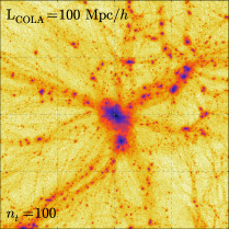
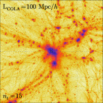
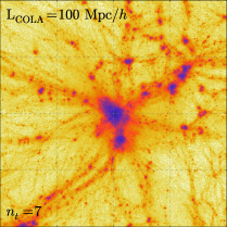
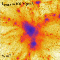
In Figure 1 we show slices through the CDM density field obtained with the original temporal COLA method666Note that we did not try to optimize the choice for for this simulation set-up as prescribed in TZE, so the results we present here using the original COLA method can be suboptimal. by setting (see Section 2.3) the full box and COLA box sizes to be the same, i.e. L Mpc. We vary the number of timesteps between 100 and 7 across the columns of that panel plot. The two rows correspond to two different magnifications: the top slices are Mpc on the side, while the bottom are Mpc. One can clearly see that the original temporal COLA method behaves as expected. It reproduces the large-scale features faithfully, while performing gradually worse at small scales when is lowered. For halos puff up significantly as the few timesteps become insufficient for the N-body side of the code to keep particles tightly bound to halos (see TZE). One can see that from Table 1 (discussed in more detail below) as well, where the central halo mass shows a gradual decline with decreasing , while the halo size increases. Note that the errors in the halo position in both real and redshift space are within kpc, while the finger-of-god (FoG) effect is consistently underestimated. For a discussion of how these imperfections can be fixed, see TZE for example.
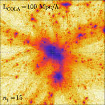
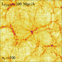
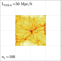
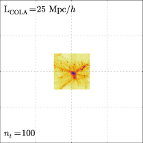
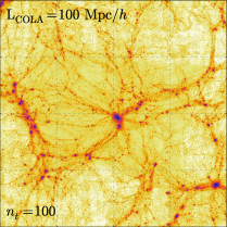
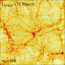
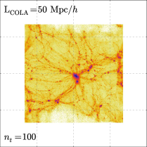
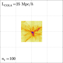
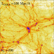
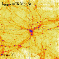
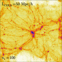
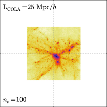
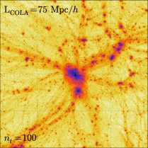
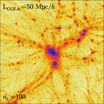
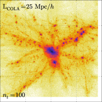
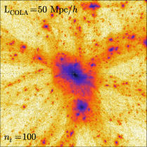
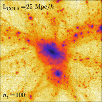
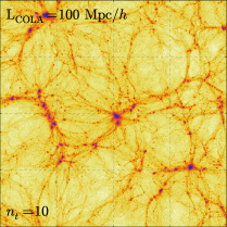
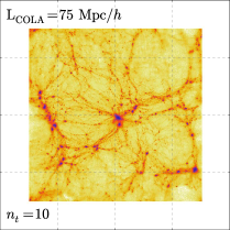
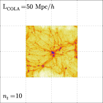
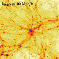
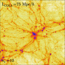
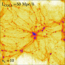
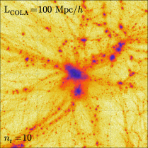
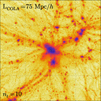
Next we focus on the simulation runs using the new sCOLA method. The results for are presented in Figure 2, while those for – in Figure 3. Columns represent different choices of COLA volume size, LCOLA, while rows represent consecutive magnifications. Concentrating on the first row of each figure, one can see how the four different simulation volumes compare in size. Inspecting the last row, one can see that the halo substructure is nearly identical across all panels with the exception of the rightmost panel (see below). Concentrating on the intermediate rows, we can see that large-scale structure is captured faithfully by sCOLA, and no large-scale distortions are introduced in the bulk even using clearly suboptimal periodic boundary conditions for the COLA volumes.
The rightmost column (L Mpc) shows clear problems: some substructure is missing, and the density field near the boundaries of the COLA volume is too smooth. The reason is straightforward to pinpoint and was already anticipated in Section 2.3. The COLA box for that run is too small to include all particles that end up in the vicinity of the central halo, thus providing an illustration of how sCOLA behaves when it is pushed beyond breaking (see Section 2.3).
It is not surprising that the snapshot with L Mpc exhibits problems. The boundary region, which is the region within Mpc from the COLA boundary, where we expect to see sCOLA misbehaving (see Section 2.3), occupies most of the volume in this
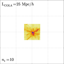
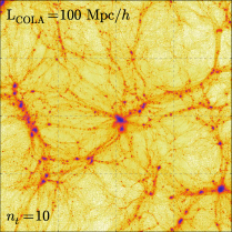
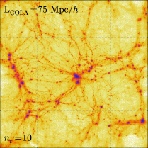
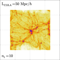
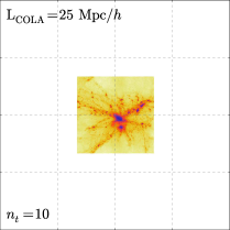
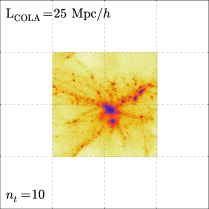

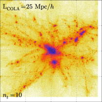
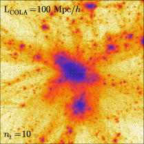

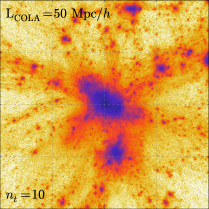
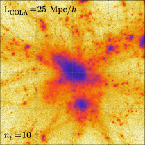
snapshot. Thus, it is only for L Mpc and above that we can expect the boundary effects on the central halo to be small, which is indeed confirmed.
Another example of sCOLA breaking is close to the COLA volume boundaries, which we again anticipated in Section 2.3. In Figures 2 and 3, one can clearly see artifacts from the non-zero and the periodic boundary conditions. Those are especially prominent on the right edge of the L Mpc COLA volume, where one can see a high-density wall of particles, which is missing from the larger COLA volume snapshots. Inspecting the larger COLA volume snapshots, we see that those particles are actually flowing to the left, outside of the central Mpc, and are therefore wrapped around by the periodic BCs in the L Mpc snapshot. Similarly, the lower COLA boundary for the same snapshot is clearly emptied out since in our pyCOLA implementation no particles from outside the COLA volume are allowed to flow in.
Nevertheless, those boundary artifacts in the L Mpc snapshot do not affect the accurate recovery of the density field in the bulk. Thus, in this example sCOLA has allowed us to reduce the simulation volume by a factor of 8 without sacrifice in the recovered central halo bulk properties, environment or substructures.
For the temporal domain behavior of sCOLA is approaching a full-blown N-body simulation. We next show how sCOLA behaves when is substantially reduced, thus making full use of the original temporal-domain COLA side of the method. Figure 3 demonstrates this feature of the method by significantly reducing both LCOLA and . As one can see, those combined sCOLA/COLA snapshots share the same pros and cons of the two methods. Thus, depending on the application, one can apply COLA independently in the spatial and temporal domains, or simultaneously, as needed.
To be more quantitative, we investigate the properties of the central halo. We ran a friends-of-friends halo finding algorithm777We use the University of Washington FOF code available here: http://www-hpcc.astro.washington.edu/tools/fof.html on all simulation snapshots presented in this paper, using a fixed linking length of 0.2. The results for the halo at the center of each snapshot are collected in Table 1. As reference values, we use the results from the most accurate simulation, corresponding to L Mpc, . Thus, the reference value for the mass of the central halo is M. In the table we list the error in the recovered halo mass relative to the reference value, the error in its center-of-mass position and velocity888For velocity, we quote values for , where is the Hubble parameter at scale factor , is conformal time, and is comoving distance. Thus, the units of our velocity variable are Mpc. This definition allows calculating redshift-space positions trivially: one simply has to add the line-of-sight velocity to the halo position. and the error in the root-mean-square (rms) of the halo particle positions, giving a measure of the halo size, as well as the error in the rms halo particle velocities, giving a measure of the FoG effect in redshift space.
In Table 1, we can see that for , sCOLA performs superbly for L Mpc and L Mpc, i.e. as long as all halo particles are captured inside the COLA volume. All errors in both real and redshift space are around or well within the force resolution, and the halo mass is recovered to 1% or better.
When is pushed down to , we see that most of the deterioration can be attributed to the smaller number of timesteps (i.e. to the original COLA method), and not to the sCOLA side of the code. That is evident when comparing the results of smaller COLA volumes to the result of the L Mpc, snapshot.
4 Summary
In this proof-of-concept paper we presented sCOLA – an extension to the N-body COLA method in the spatial domain. sCOLA is a straightforward modification to N-body codes, which uses perturbation theory to calculate the far field potential from masses outside a region of interest, while solving for the near field using an N-body code. The use of perturbation theory allows for the N-body side of sCOLA to perform all calculations entirely within the region of interest (dubbed the “COLA volume”), without the need to substantially increase the simulated volume to capture the effects of large modes or structures outside that region.
Compared to standard zoom-in simulation methods, the main advantage of sCOLA is that it makes the different volumes completely independent once the initial conditions are computed. Thus, there is no need to add lower resolution zones around the region of interest in sCOLA.
The sCOLA method leads to the exact equations of motion when the COLA volume coincides with the full volume, capturing all large-scale modes affecting the region of interest. When the COLA volume does not cover the full volume, the approximations behind sCOLA require one to run the N-body code behind sCOLA on a region which is roughly 10 Mpc larger in all directions than the region of interest.
We demonstrated the usage of sCOLA by showing results from zoom-in simulations performed with a freely available sCOLA-based N-body code (called pyCOLA), which we developed for this paper. Our results demonstrate that sCOLA faithfully recovers large-scale structure inside a COLA volume as small as 50 Mpc (possibly even smaller), while keeping substructures intact. Moreover, we showed that sCOLA can be safely used in conjunction with the original COLA method. We find that reducing the number of timesteps for COLA naturally degrades the quality of the simulation. However, the sCOLA-side of the method proves robust to reducing the size of the COLA box until the COLA boundary region (at redshift zero, corresponding to the region Mpc or less from the edge) invades the region of interest.
An immediate application of sCOLA is as a method for performing zoom-in simulations, which we illustrated in this paper. The fact that the N-body side of sCOLA is needed to perform calculations of the potential only for the near field, implies that sCOLA-based N-body codes can be made embarrassingly parallel, thus opening the door for efficiently tiling a volume of interest using grid computing in what may become Cosmology@Home. Moreover, combining sCOLA with the original COLA method can be useful for cheaply generating large ensembles of accurate mock halo catalogs required to study uncertainties of large-scale structure observables. Surveys with large aspect ratios, such as pencil-beam surveys, can especially benefit, as sCOLA can easily capture the effects of large-scale transverse modes without the need to substantially increase the simulated volume.
pyCOLA can be found on the following URL: https://bitbucket.org/tassev/pycola/.
Acknowledgments
ST would like to thank his colleagues and students at Braintree High School for making his entrance into public high school teaching a rewarding and joyful experience. M.Z. is supported in part by NSF Grants No. PHY-1213563 and No. AST-1409709.
Appendix A The details behind sCOLA
In this appendix we write down the exact first equation of the sCOLA algorithm, given schematically by eq. (2.4). One should read this appendix as a continuation of Appendix A of TZE. The preliminaries, notation, and original temporal-domain COLA (tCOLA) are presented there. Here we present the modifications to the original tCOLA method needed to extend COLA to the spatial domain.
A.1 The sCOLA method
The COLA method (both tCOLA and sCOLA) dictates that we integrate the equation of motion for CDM particles in a frame comoving with observers following trajectories specified by LPT. Thus, we solve for the residual displacement of CDM particles:
| (A.1) |
For tCOLA, the equation of motion is written as (see eq. A.6 in TZE)
| (A.2) |
For sCOLA, we rewrite it as
| (A.3) |
Thus, the only difference between sCOLA and tCOLA is adding the COLA superscript where appropriate, reminding us that those quantities are calculated in the small COLA box, covering only a fraction of the original volume. The calculation of the LPT displacement fields, , in the COLA box is presented in Appendix B.
Below we present results for the combined tCOLA/sCOLA discretization as employed in pyCOLA. Therefore, as described in TZE, next we discretize the operator only on the left-hand side of the above equation, using as a velocity variable , which is the CDM velocity as measured by an LPT observer.
A.2 Discretizing in sCOLA in the standard approach
Similar to TZE, we discretize the sCOLA equations using a kick-drift-kick scheme. That requires writing down a kick operator , a drift operator , as well as introducing two more operators, , for converting between the standard particle velocity and the residual velocity as measured by LPT observers.
In the “standard” prescription (see A.3.1 of TZE), the operators and of tCOLA and sCOLA are identical. The kick operator in sCOLA, however, is modified (compare with eq. A.7 of TZE):
where as in TZE we dropped the subscript from for brevity.
Time evolution between and in sCOLA is achieved in exactly the same way as in tCOLA, by applying the following operator on :
| (A.5) |
As in TZE, here we defined
| (A.6) |
which as mentioned above, first transforms the initial conditions for to the rest frame of LPT observers (), and then adds back the LPT velocities at the end ().
A.3 Modified discretization of in sCOLA
As done in Appendix A.3.2 of TZE, here we present a modified discretization scheme of , which allows one to improve the convergence properties of COLA. As above, the and operators of tCOLA and sCOLA in this scheme are identical. The kick operator in sCOLA, however, is modified (compare with eq. A.15 of TZE):
where we again dropped the subscript from for brevity. The equations presented above give the evolution equations behind the sCOLA algorithm presented in this paper.
However, in practice, we found that using the above prescription results in density fields from sCOLA which are artificially smoothed. The reason is due to a mismatch at very short scales between the LPT displacement fields calculated in the sCOLA box and the original simulation volume. Such a mismatch at deeply non-linear scales has no deep physical origin and we view it as an artifact of the different algorithms we use for calculating the LPT fields, combined with numerical precision issues. Removing that artifact is trivial: we boxcar average999For different simulation set-ups, one may need to experiment with varying the boxcar window, or using a Gaussian averaging instead. (with width of 2 particle cells) all LPT displacement fields entering the operators , and . That eliminates most short-scale noise, which otherwise artificially smoothed our final results. We would like to emphasize that no information is lost in such an averaging as LPT carries little (if any) information on the scale of the averaging window we chose. Moreover, the convergence of our scheme to the “truth” when the number of timesteps and sCOLA volume are brought to infinity is not affected since in that case we would add and subtract the same averaged LPT displacements. Note that the averaging is done only on the displacements entering the evolution operators, and not on the initial conditions, as we want to keep the initial conditions intact.
Appendix B Calculating LPT displacements using force evaluations
In this appendix we write down the exact second equation of the sCOLA algorithm, given schematically by eq. (2.5), and describe how we solve it in pyCOLA. The non-schematic version of equation (2.5) reads:
where .
The usual way to derive the LPT displacement fields, and , is using Fourier techniques [27]. However, the method we employ is based on [28], where the equation above is solved in real space by calculating the gravitational forces due to the density field entering above at early enough times that one can consider the results perturbative. The right-hand side above is completely determined by the initial conditions in the full volume. So, all we need to do is extract its first- and second-order pieces and match those to the corresponding terms on the left-hand side. We do that explicitly below, following [28]. This is advantageous in our case because the displacement fields in the equation above live in two separate boxes – the COLA box () and the full box (). The results are summarized below, and are implemented in the public pyCOLA code. These results include modifications to [28] (allowing in the notation below) to obtain high-precision LPT displacements for the sCOLA box. For further information, see [28].
pyCOLA offers a choice in the calculation of the first-order and second-order displacements, , in the COLA volume, as well as in the full volume at redshift zero: using a 2-pt or a 4-pt (denoted by superscript) rule. Depending on the rule, the first/second order displacements receive higher-order corrections as follows: at third/fourth order when using the 2pt rule; at fifth/sixth order when using the 4pt rule. The displacement fields are given by ( below stands for the displacement field in the COLA box or the full box):
| (B.2) | |||||
where
| (B.3) |
and and are arbitrary constants. The equations above become exact in the limit of , . When writing the equations above in the COLA box to second order (i.e. ), one must use in order to be consistent in PT. If one wants to use the above equations for calculating in the full box, then one must set since requires one to provide . The factors of ( being the matter density today) are needed to rescale the second order displacements to matter domination and are correct to in .
The force corresponds to the right-hand side of eq. (B). It is evaluated numerically by using the force calculation function (using a 4-pt finite difference scheme) of pyCOLA on the PM grid. Analytically, is given by:
| (B.4) |
where and correspond to the first and second order growth factors, assumed to be deep in matter domination (see the arguments of in eq. (B) above).
The fractional overdensity, , in pyCOLA is calculated using cloud-in-cell assignment from a grid of particles (at Lagrangian positions ) displaced by the first and second order displacement fields: . Note that implicitly for each particle at Lagrangian position , the force is evaluated at its corresponding Eulerian position: . The choice of ( or =“full”) determines which particles (only those in the COLA volume, or all particles in the full volume) are included in the calculation of the potential, .
References
- [1] J. J. M. Carrasco, M. P. Hertzberg, and L. Senatore, The effective field theory of cosmological large scale structures, Journal of High Energy Physics 9 (Sept., 2012) 82, [arXiv:1206.2926].
- [2] J. Carlson, B. Reid, and M. White, Convolution Lagrangian perturbation theory for biased tracers, MNRAS 429 (Feb., 2013) 1674–1685, [arXiv:1209.0780].
- [3] R. A. Porto, L. Senatore, and M. Zaldarriaga, The Lagrangian-space Effective Field Theory of large scale structures, JCAP 5 (May, 2014) 22, [arXiv:1311.2168].
- [4] R. Scoccimarro and R. K. Sheth, PTHALOS: a fast method for generating mock galaxy distributions, MNRAS 329 (Jan., 2002) 629–640, [astro-ph/0106120].
- [5] M. Manera, R. Scoccimarro, W. J. Percival, L. Samushia, C. K. McBride, A. J. Ross, R. K. Sheth, M. White, B. A. Reid, A. G. Sánchez, R. de Putter, X. Xu, A. A. Berlind, J. Brinkmann, C. Maraston, B. Nichol, F. Montesano, N. Padmanabhan, R. A. Skibba, R. Tojeiro, and B. A. Weaver, The clustering of galaxies in the SDSS-III Baryon Oscillation Spectroscopic Survey: a large sample of mock galaxy catalogues, MNRAS (Oct., 2012) 118, [arXiv:1203.6609].
- [6] S. Tassev, M. Zaldarriaga, and D. J. Eisenstein, Solving large scale structure in ten easy steps with COLA, JCAP 6 (June, 2013) 36, [arXiv:1301.0322].
- [7] F. Leclercq, J. Jasche, H. Gil-Marín, and B. Wandelt, One-point remapping of Lagrangian perturbation theory in the mildly non-linear regime of cosmic structure formation, JCAP 11 (Nov., 2013) 48, [arXiv:1305.4642].
- [8] P. Monaco, E. Sefusatti, S. Borgani, M. Crocce, P. Fosalba, R. K. Sheth, and T. Theuns, An accurate tool for the fast generation of dark matter halo catalogues, MNRAS 433 (Aug., 2013) 2389–2402, [arXiv:1305.1505].
- [9] M. White, J. L. Tinker, and C. K. McBride, Mock galaxy catalogues using the quick particle mesh method, MNRAS 437 (Jan., 2014) 2594–2606, [arXiv:1309.5532].
- [10] F.-S. Kitaura, H. Gil-Marín, C. Scoccola, C.-H. Chuang, V. Müller, G. Yepes, and F. Prada, Constraining the halo bispectrum in real and redshift space from perturbation theory and non-linear stochastic bias, ArXiv e-prints (July, 2014) [arXiv:1407.1236].
- [11] S. Avila, S. G. Murray, A. Knebe, C. Power, A. S. G. Robotham, and J. Garcia-Bellido, HALOGEN: A new tool for fast generation of mock halo catalogues, ArXiv e-prints (Dec., 2014) [arXiv:1412.5228].
- [12] C.-H. Chuang, F.-S. Kitaura, F. Prada, C. Zhao, and G. Yepes, EZmocks: extending the Zel’dovich approximation to generate mock galaxy catalogues with accurate clustering statistics, MNRAS 446 (Jan., 2015) 2621–2628, [arXiv:1409.1124].
- [13] C.-H. Chuang, C. Zhao, F. Prada, E. Munari, S. Avila, A. Izard, F.-S. Kitaura, M. Manera, P. Monaco, S. Murray, A. Knebe, C. G. Scoccola, G. Yepes, J. Garcia-Bellido, F. A. Marin, V. Muller, R. Skibba, M. Crocce, P. Fosalba, S. Gottlober, A. A. Klypin, C. Power, C. Tao, and V. Turchaninov, nIFTy Cosmology: Galaxy/halo mock catalogue comparison project on clustering statistics, ArXiv e-prints (Dec., 2014) [arXiv:1412.7729].
- [14] E. A. Kazin, J. Koda, C. Blake, N. Padmanabhan, S. Brough, M. Colless, C. Contreras, W. Couch, S. Croom, D. J. Croton, T. M. Davis, M. J. Drinkwater, K. Forster, D. Gilbank, M. Gladders, K. Glazebrook, B. Jelliffe, R. J. Jurek, I.-h. Li, B. Madore, D. C. Martin, K. Pimbblet, G. B. Poole, M. Pracy, R. Sharp, E. Wisnioski, D. Woods, T. K. Wyder, and H. K. C. Yee, The WiggleZ Dark Energy Survey: improved distance measurements to z = 1 with reconstruction of the baryonic acoustic feature, MNRAS 441 (July, 2014) 3524–3542, [arXiv:1401.0358].
- [15] C. Howlett, A. J. Ross, L. Samushia, W. J. Percival, and M. Manera, The Clustering of the SDSS Main Galaxy Sample II: Mock galaxy catalogues and a measurement of the growth of structure from Redshift Space Distortions at $z=0.15$, ArXiv e-prints (Sept., 2014) [arXiv:1409.3238].
- [16] A. J. Ross, L. Samushia, C. Howlett, W. J. Percival, A. Burden, and M. Manera, The Clustering of the SDSS DR7 Main Galaxy Sample I: A 4 per cent Distance Measure at z=0.15, ArXiv e-prints (Sept., 2014) [arXiv:1409.3242].
- [17] F. Leclercq, J. Jasche, P. M. Sutter, N. Hamaus, and B. Wandelt, Dark matter voids in the SDSS galaxy survey, ArXiv e-prints (Oct., 2014) [arXiv:1410.0355].
- [18] F. Leclercq, J. Jasche, and B. Wandelt, Bayesian analysis of the dynamic cosmic web in the SDSS galaxy survey, ArXiv e-prints (Feb., 2015) [arXiv:1502.02690].
- [19] F. R. Bouchet, S. Colombi, E. Hivon, and R. Juszkiewicz, Perturbative Lagrangian approach to gravitational instability., A&A 296 (Apr., 1995) 575, [astro-ph/9406013].
- [20] S. Tassev, Lagrangian or Eulerian; real or Fourier? Not all approaches to large-scale structure are created equal, JCAP 6 (June, 2014) 8, [arXiv:1311.4884].
- [21] J. Carlson and M. White, Embedding Realistic Surveys in Simulations Through Volume Remapping, ApJS 190 (Oct., 2010) 311–314, [arXiv:1003.3178].
- [22] R. E. Angulo and S. D. M. White, One simulation to fit them all - changing the background parameters of a cosmological N-body simulation, MNRAS 405 (June, 2010) 143–154, [arXiv:0912.4277].
- [23] M. D. Schneider, S. Cole, C. S. Frenk, and I. Szapudi, Fast Generation of Ensembles of Cosmological N-body Simulations Via Mode Resampling, ApJ 737 (Aug., 2011) 11, [arXiv:1103.2767].
- [24] O. Hahn and T. Abel, Multi-scale initial conditions for cosmological simulations, MNRAS 415 (Aug., 2011) 2101–2121, [arXiv:1103.6031].
- [25] A. Jenkins, A new way of setting the phases for cosmological multiscale Gaussian initial conditions, MNRAS 434 (Sept., 2013) 2094–2120, [arXiv:1306.5968].
- [26] S. Tassev and M. Zaldarriaga, Estimating CDM particle trajectories in the mildly non-linear regime of structure formation. Implications for the density field in real and redshift space, JCAP 12 (Dec., 2012) 11, [arXiv:1203.5785].
- [27] M. Crocce, S. Pueblas, and R. Scoccimarro, Transients from initial conditions in cosmological simulations, MNRAS 373 (Nov., 2006) 369–381, [astro-ph/0606505].
- [28] L. Garrison et al. To appear.