Tracking an Object with Unknown Accelerations using a Shadowing Filter

Abstract

A commonly encountered problem is the tracking of a physical object, like a maneuvering ship, aircraft, land vehicle, spacecraft or animate creature carrying a wireless device. The sensor data is often limited and inaccurate observations of range or bearing. This problem is more difficult than tracking a ballistic trajectory, because an operative affects unknown and arbitrarily changing accelerations. Although stochastic methods of filtering or state estimation (Kalman filters and particle filters) are widely used, out of vogue variational methods are more appropriate in this tracking context, because the objects do not typically display any significant random motions at the length and time scales of interest. This leads us to propose a rather elegant approach based on a shadowing filter. The resulting filter is efficient (reduces to the solution of linear equations) and robust (uneffected by missing data and singular correlations that would cause catastrophic failure of Bayesian filters.) The tracking is so robust, that in some common situations it actually performs better by ignoring error correlations that are so vital to Kalman filters.

1 Introduction

The literature on tracking of isolated or multiple objects in uncluttered and cluttered environments is broad and varied, with methodological approaches ranging from variational techniques to an extensive variety of Kalman filters, particles filters, and other sequential Bayesian filters [1, 3, 7, 10].

Optimal tracking (filtering or state estimation) requires identification of the appropriate length and time scales of a object’s motion, and the magnitudes of the uncertainty (observational and dynamical noise) and the nonlinearity at these scales. There are three broad scenarios: (1) when the update cycle is fast, such in guidance control, Kalman filters are appropriate, because system behaviours are almost linear; (2) when nonlinearity is significant, and the noise largely dynamical, as opposed to observational, then particle filters are appropriate; and (3) when nonlinearity is significant, but the noise largely observational, then variational methods are most appropriate. Mathematically situations (1) and (2) best assume the underlying process is stochastic, whereas situation (3) it is best to assume a deterministic dynamical system: the success and universal acceptance of stochastic methods, over the past decades, has lead to them being applied in situation (3), where they are not the most appropriate choice [9].

Here we present an approach to tracking in situation (3) based on shadowing filters, which derive from the modern concept of shadowing in dynamical systems theory; literally meaning to find a trajectory that shadows the observations [6]. The methodology has its roots in the work of Laplace and Gauss fitting celestial orbits as curves [4], and subsequent least squares approaches for ballistic trajectories. Shadowing filters lie within the domain of variational methods, as in optimal control, but are subtly different [8]. Shadowing filters are not equivalent to 4D-variational assimilation often employed in meteological and oceanographic modelling and forecasting. Nor are they equivalent to dynamic programming approaches that finds a Viterbi path [5].

To develop our methodology, a one-dimensional, or scalar case, is considered first, which is then extended to the multi-dimensional vector case, where the observations are of the components of the Cartesian position vector. From this basis other relevant observation situations that are often encountered are considered, for example, using range or bearing observations from one or more sensors. A significant problem that arises in these types of observation networks is the way the covariance of observational errors varies with position, in particular, the singularities that occur when the target and sensors are co-linear or co-planar. Possibly the most surprising outcome of the shadowing filter approach is that singular covariances of observations are not a significant problem, and targets can be tracked through missing data and singularities relatively easily; indeed, sometimes covariances can be ignored entirely, obtaining very efficient tracking filters.

To keep the exposition of the algorithm and its benefits clear, we restrict attention to tracking an isolated vehicle in an uncluttered environment. It should be clear, once the methodology is understood, that since the shadowing filter assumes a tracked object maintains a contiguous trajectory it will perform well with multiple targets in cluttered environments.

2 Formulation and implementation

2.1 Scalar case

Our initial interest is tracking the position of a point object in one dimension, given a sequence of noisy observations. Let $\mathcal{P}_{i}\in\mathbb{R}$ be the observed position at time $t_{i}$ for $i=0,\dots,n$, and $\sigma_{i}^{2}$ be the variance of the observational error. The object’s dynamics are modelled by its position $p_{i}\in\mathbb{R}$ and velocity $v_{i}\in\mathbb{R}$ at $t_{i}$, and constant acceleration $a_{i}\in\mathbb{R}$ for $t_{i}\leq{}t<t_{i+i}$. For notational convenience, define $\tau_{i}=t_{i+1}-t_{i}$. Our goal is to have $p_{i}$ close to $\mathcal{P}_{i}$ subject to the accelerations not being excessively large or changeable. We might therefore choose to minimise the total square error $\sum_{i=0}^{n}\sigma_{i}^{-2}(\mathcal{P}_{i}-p_{i})^{2}$ subject to accelerations over the interval being bounded, $a_{i}^{2}\leq\xi^{2}$ $i=0,\dots,n-1$. Bounded acceleration is an appropriate constraint, but it introduces technical difficulties. Although these difficulties can be over-come [8], it is more convenient and efficient to instead constrain the root mean squared acceleration over the entire trajectory, $\sum_{i=0}^{n-1}\tau_{i}a_{i}^{2}\leq{}(t_{n}-t_{0})\xi^{2}$.

Assuming Newton’s laws and Galilean transforms apply to the point object’s motion, then the stated optimisation problem can be posed using a Lagrangian:

$$L =\frac{1}{2}\sum_{i=0}^{n}\sigma_{i}^{-2}(\mathcal{P}_{i}-p_{i})^{2}$$ (1)

$$+\sum_{i=0}^{n-1}\lambda_{i}(p_{i+1}-p_{i}-v_{i}\tau_{i}-\frac{1}{2}a_{i}\tau_{i}^{2})$$ (2)

$$+\sum_{i=0}^{n-1}\mu_{i}(v_{i+1}-v_{i}-a_{i}\tau_{i})$$ (3)

$$+\eta\left(\sum_{i=0}^{n-1}\tau_{i}a_{i}^{2}-(t_{n}-t_{0})\xi^{2}\right),$$ (4)

where $\lambda_{i}\in\mathbb{R}$, $\mu_{i}\in\mathbb{R}$ and $\eta\geq 0$ are dual variables. Solving the optimisation, and defining

$$p(t)=p_{i}+v_{i}(t-t_{i})+\frac{1}{2}a_{i}(t-t_{i})^{2}\quad\text{for}\quad t_{i}\leq t\leq t_{i+1},$$ (5)

provides an optimal quadratic spline estimate of a particle’s path assuming piecewise constant accelerations. The optimal solution occurs where all the partial derivatives of $L$ are zero:

$$\frac{\partial L}{\partial p_{i}} =\left.\begin{cases}-\sigma_{0}^{-2}(\mathcal{P}_{0}-p_{0})-\lambda_{0},&i=0,\\ -\sigma_{i}^{-2}(\mathcal{P}_{i}-p_{i})+\lambda_{i-1}-\lambda_{i},&0<i<n,\\ -\sigma_{n}^{-2}(\mathcal{P}_{n}-p_{n})+\lambda_{n-1},&i=n,\\ \end{cases}\right\}=0$$ (6)

$$\frac{\partial L}{\partial v_{i}} =\left.\begin{cases}-\lambda_{0}\tau_{0}-\mu_{0},&i=0,\\ -\lambda_{i}\tau_{i}+\mu_{i-1}-\mu_{i},&0<i<n,\end{cases}\right\}=0$$ (7)

$$\frac{\partial L}{\partial a_{i}} =-\frac{1}{2}\lambda_{i}\tau_{i}^{2}-\mu_{i}\tau_{i}+2\eta{}\tau_{i}a_{i}=0,$$ (8)

$$\frac{\partial L}{\partial\lambda_{i}} =p_{i+1}-p_{i}-v_{i}\tau_{i}-\frac{1}{2}a_{i}\tau_{i}^{2}=0,$$ (9)

$$\frac{\partial L}{\partial\mu_{i}} =v_{i+1}-v_{i}-a_{i}\tau_{i}=0,$$ (10)

$$\frac{\partial L}{\partial\eta} =\sum_{i=0}^{n-1}\tau_{i}a_{i}^{2}-(t_{n}-t_{0})\xi^{2}=0.$$ (11)

Equation (6) is defined for $0\leq{}i\leq{}n$ while (7–10) are defined for $0\leq{}i<n-1$. With the exception of (11), the remaining five equations are linear in the unknowns. However, $\xi$ and $\eta$ are related through term (4) of the Lagrangian, which is the only place they appear. Hence, one can solve the linear equations (6–10) for a fixed $\eta$, then compute the corresponding value of $\xi$ from eq. (11). The optimal solution for any $\xi$ can be approximated arbitrarily closely by an efficient one-dimensional search, such as Brent’s method [11]. In practice it is unlikely that $\xi$ needs to be specified precisely, after all, it is only a bound on the root mean squared acceleration. Consequently, it is usually sufficient to work only with $\eta$, treating it as a smoothing, or regularisation, parameter.

Combining (9) and (10) to eliminate the $v_{i}$ gives

$$p_{i+1}\tau_{i-1}-p_{i}(\tau_{i}+\tau_{i-1})+p_{i-1}\tau_{i}=\frac{1}{2}(a_{i}\tau_{i}+a_{i-1}\tau_{i-1})\tau_{i-1}\tau_{i},$$ (12)

for $0<i<n$. Combining (6), (7) and (8) and eliminating the dual variables $\lambda_{i}$ and $\mu_{i}$ (as explained in the following), obtains another set of expressions relating the $p_{i}$ and $a_{i}$, which when combined with (12) enable solving for a near optimal solution very efficiently.

There is a certain amount of redunancy in the equations just stated, but to assist formulation of a solution using matrix notation it is advantageous to retain the redundancy.

Define column vectors $\mathcal{P}=(\mathcal{P}_{0},\dots,\mathcal{P}_{n})^{T}\in\mathbb{R}^{n+1}$, $p=(p_{0},\dots,p_{n})^{T}\in\mathbb{R}^{n+1}$, $\lambda=(\lambda_{0},\dots,\lambda_{n-1})^{T}\in\mathbb{R}^{n}$, $\mu=(\mu_{0},\dots,\mu_{n-1})^{T}\in\mathbb{R}^{n}$, and finally $a=(a_{0},\dots,a_{n-1})^{T}\in\mathbb{R}^{n}$. Define $\tau$ to be the $n\times{}n$ matrix of zeros with main diagonal $(\tau_{0},\dots,\tau_{n-1})$, and $\mathcal{I}$ to be the $(n+1)\times(n+1)$ matrix of zeros with main diagonal $(\sigma_{0}^{-2},\dots,\sigma_{n}^{-2})$. Define a $n\times{}n$ matrix $D$ to have all entries zero except $-1$ on the main diagonal and $1$ on the first lower diagonal, and similarly define a $(n+1)\times{}n$ matrix $E$: specifically

$$D_{ij}=E_{ij}=\begin{cases}-1,&i=j,\\ \phantom{-}1,&i=j+1,\\ \phantom{-}0,&\text{otherwise,}\end{cases}$$ (13)

when the entry is defined. It follows that the linear equations (6), (7) and (8) can be succinctly expressed as

$$E\lambda=\mathcal{I}(\mathcal{P}-p),\qquad D\mu=\tau\lambda,\qquad 2\eta\tau{}a=\frac{1}{2}\tau^{2}\lambda+\tau\mu.$$ (14)

In the last of the three equations of (14), $\tau$ is invertible, so that a $\tau$ factor can be canceled on the left of each term.

Define a $n\times{}n$ matrix $L$, and $n\times{}(n+1)$ matrix $M$, to have a lower triangular form:

$$L_{ij}=M_{ij}=\begin{cases}-1,&i\geq{}j,\\ \phantom{-}0,&\text{otherwise,}\end{cases}$$ (15)

when the entry is defined. It can be easily verified that $DL=I$ and $EM=J$ where $I$ is the $n\times{}n$ identity matrix, and $J$ is a $(n+1)\times(n+1)$ matrix with

$$J_{ij}=\begin{cases}\phantom{-}1,&i=j\text{ and }i\neq{}n+1,\\ -1,&i=n+1\text{ and }j\neq{}n+1,\\ \phantom{-}0,&\text{otherwise.}\end{cases}$$ (16)

The identities $DL=I$ and $D\mu=\tau\lambda$ imply $\mu=L\tau\lambda$. The identities $EM=J$ and $E\lambda=\mathcal{I}(\mathcal{P}-p)$ imply that $\lambda=M\mathcal{I}(\mathcal{P}-p)$ and $\sum_{i=0}^{n-1}\sigma_{i}^{-2}(\mathcal{P}_{i}-p_{i})=0$. It follows, by substitution into the last equation of (14), that

$$2\eta{}a=\left(\frac{1}{2}\tau{}M+L\tau{}M\right)\mathcal{I}(\mathcal{P}-p),$$ (17)

which can be combined with (12) as follows. Define $(n-1)\times{}(n+1)$ matrices $A$ and $B$, and $(n-1)\times{}n$ matrix $G$:

$$G_{ij}=\begin{cases}\tau_{i}^{2}\tau_{i+1},&i=j,\\ \tau_{i}\tau_{i+1}^{2},&i+1=j,\\ \phantom{}0,&\text{otherwise,}\end{cases}$$ (18)

$$B_{ij}=\begin{cases}\tau_{i+1},&i=j,\\ -(\tau_{i}+\tau_{i+1}),&i+1=j,\\ \tau_{i},&i+2=j,\\ 0,&\text{otherwise,}\end{cases}$$ (19)

$$A=\frac{1}{4}G\left(\frac{1}{2}\tau{}M+L\tau{}M\right).$$ (20)

Then (12) can be written $Bp=\frac{1}{2}Ga$, which when combined with (17) obtains the equation

$$(A\mathcal{I}+\eta{}B)p=A\mathcal{I}\mathcal{P},$$ (21)

and the additional constraint $\sum_{i=0}^{n-1}\sigma_{i}^{-2}(\mathcal{P}_{i}-p_{i})=0$. For stability reasons discussed in section 2.3, this constraint will be extended to $\sum_{i=0}^{n}\sigma_{i}^{-2}(\mathcal{P}_{i}-p_{i})=0$. Defining a $n\times{}(n+1)$ matrix $\boldsymbol{\underline{B}}$ to be $B$ augmented with a final row of zeros, and a $n\times{}(n+1)$ matrix $\boldsymbol{\underline{A}}$ to be $A$ augmented with a final row of ones, then

$$\left(\boldsymbol{\underline{A}}\mathcal{I}+\eta\boldsymbol{\underline{B}}\right)p=\boldsymbol{\underline{A}}\mathcal{I}\mathcal{P},$$ (22)

encodes both (21) and the extended constraint. Solving (22) by singular value decomposition obtains a least squares approximate solution for the position $p$ for given smoothing parameter $\eta$. See section 2.3 on the nature of this approximation and the optimal presentation of the data in $\mathcal{P}$. It is important to read section 2.3 before implementing (22).

2.2 Vector case

Consider now the situation where a point vehicle is positioned in a $d$-dimensional Euclidean space with Cartesian coordinates. Suppose that the coordinate positions are observed as a sequence $\mathcal{P}_{i}\in\mathbb{R}^{d}$ in such a way that the observational errors have a $d\times{}d$ covariance matrix $\mathcal{C}_{i}$, and corresponding information matrix $\mathcal{I}_{i}=\mathcal{C}_{i}^{-1}$. The quantities to be determined are $p_{i}\in\mathbb{R}^{d}$, $v_{i}\in\mathbb{R}^{d}$, and $a_{i}\in\mathbb{R}^{d}$, which are all now $d$-dimensional column vectors. If the aim is to track the trajectory under the assumption of bounded RMS magnitude of the acceleration, the Lagrangian (1) now becomes vectorised as

$$L = \frac{1}{2}\sum_{i=0}^{n}(\mathcal{P}_{i}-p_{i})^{T}\mathcal{I}_{i}(\mathcal{P}_{i}-p_{i})$$ (26)

$$+\sum_{i=0}^{n-1}\lambda_{i+1}^{T}(p_{i+1}-p_{i}-v_{i}\tau_{i}-\frac{1}{2}a_{i}\tau_{i}^{2})$$

$$+\sum_{i=0}^{n-1}\mu_{i+1}^{T}(v_{i+1}-v_{i}-a_{i}\tau_{i})$$

$$+\eta\left(\sum_{i=0}^{n-1}\tau_{i}a_{i}^{T}a_{i}-(t_{n}-t_{0})\xi^{2}\right),$$

where $\lambda_{i}\in\mathbb{R}^{d}$, $\mu_{i}\in\mathbb{R}^{d}$ are now $d$-dimensional column vectors, but $\eta\in\mathbb{R}$. The superscript $T$ indicates the transpose.

The solution of the vectorised optimization problem proceeds identically to the scalar case, using the same linear algebra methods. Let $\mathcal{P}\in\mathbb{R}^{d(n+1)}$ denote a column vector being the time-series of $n+1$ observations $\mathcal{P}_{i}\in\mathbb{R}^{d}$ stacked in $d$-dimensional blocks, and similarly for position variables $p\in\mathbb{R}^{d(n+1)}$. Let $\mathcal{I}$ denote the $(n+1)d\times(n+1)d$ block diagonal matrix with the $d\times{}d$ information matrices $\mathcal{I}_{i}$ along the diagonal. Finally, let $I_{d}$ denotes the $d\times{}d$ identity matrix and let $\widehat{M}=M\otimes{}I_{d}$ denote the outer product of an arbitrary matrix $M$ with $I_{d}$, that is, $\widehat{M}$ has a block structure where each scalar entry $M_{ij}$ of $M$ becomes a $d\times{}d$-block $M_{ij}I_{d}$ of $\widehat{M}$. Then the vectorised solution is

$$\left(\boldsymbol{\underline{\widehat{A}}}\mathcal{I}+\eta\boldsymbol{\underline{\widehat{B}}}\right)p=\boldsymbol{\underline{\widehat{A}}}\mathcal{I}\mathcal{P}.$$ (27)

2.3 Implementation and interpretation of the filter

Solving (22) or (27) obtains an approximate solution to the optimal shadowing trajectory for a given smoothness $\eta$. To see this, note that the system of equations (22) is under-determined: there are $n$ linear equations in $n+1$ unknowns. This occurs because in deriving (12) the velocity variables were eliminated, but to completely define a trajectory the velocity needs to be known at some time; usually the initial or final velocity is specified or solved for. To solve for the velocity requires introducing another $n$ variables and $n$ equations to solve for all the velocities, which is significant additional computation for very little benefit. The approximation (22) relies on the fact that if the time window of the trajectory is sufficiently long, then accurate specification of the initial velocity is not required. It just means the initial part of the trajectory may not accurately fit the observations. However, leaving the initial velocity unspecified can lead to instability for short time windows. Imposing the extended constraint $\sum_{i=0}^{n}\sigma_{i}^{-2}(\mathcal{P}_{i}-p_{i})=0$ overcomes possible instability by implicitly defining an initial velocity.

In formulating the Lagrangian forward differences were used to express position in terms of velocity and acceleration. Unfortunately, this results in $A$ and $B$ having a lower triangular form. Consequently, the approximation errors are largest for the $p_{i}$ with largest $i$, which is not what is wanted for state estimation and forecasting; it is preferable that the smallest errors are at the most recent times. Reformulating the Langrangian with backward differences solves this problem, however, there is much simpler solution: initially reversing the time-series data sequence $(\tau_{i},\mathcal{P}_{i},\mathcal{I}_{i})$, applying the filter (22) or (27), then reversing shadowing trajectory time-series $p_{i}$ to obtain the desired result. Even this trick is unnecessary. Let $R$ denote the matrix that reverses a vector, then the time-series reversal trick, is equivalent to changing (21) to

$$\left(A\mathcal{I}+\eta{}B\right)Rp=AR\mathcal{I}\mathcal{P},$$ (28)

but since $R^{-1}=R$, multipling on the left by $R$ obtains

$$\left(RAR\mathcal{I}+\eta{}RBR\right)p=RAR\mathcal{I}\mathcal{P},$$ (29)

where the matrices $RAR$ and $RBR$ are just $A$ and $B$ with their rows and columns reversed. Hence, the time-reversal trick is some bookkeeping when constructing $A$ and $B$.

3 Illustrative examples

This section provides demonstrations of the use of the proposed methods. The scalar filter is considered first, both as an off-line smoothing filter and sequential state-estimator. The vector filter is considered for observations in cartesian coordinates, with and without correlation, which is a preliminary to section 4 where non-cartesian observations are considered.

3.1 Scalar filter for moothing and sequential tracking

Here tracking of one observed variable is examined for increasing values of smoothing paramter $\eta$. The filter is employed as smoothing filter over the entire observation window, and as a sequential state-estimator. In both cases the time-reversal trick discussed in section 2.3 is employed. In this example employs a large red noise component $\chi_{t}$ to mimic a vehicle maneuvering in an unpredictable way.

Figure 1: Position tracking $25+10\sin(t/15)+\chi_{t}+3\epsilon_{t}$, $0\leq{}t\leq{}100$ where $\epsilon_{t}$ is a white noise process $N(0,1)$, and $\chi_{t}$ an independent cumulative of a white noise process $N(0,1)$. Shadowing filter results for smoothing parameters as stated.

Figure 2: Computed accelerations for tracking shown in fig. 1 for selected $\eta$. Accelerations are scaled by $\sqrt{\eta}$ to allow easier comparision.

Figure 3: Sequential tracking of same data as shown in fig. 1 for selected $\eta$. State estimates use only observations up to that time, and final filtered state at that time is plotted.

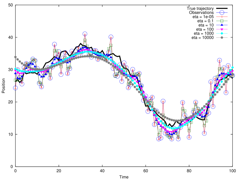
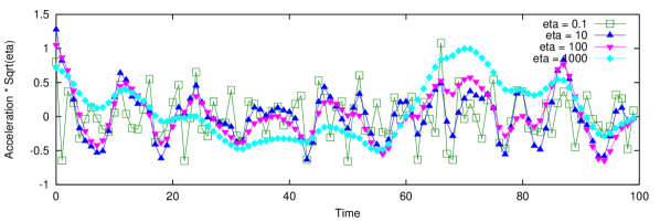
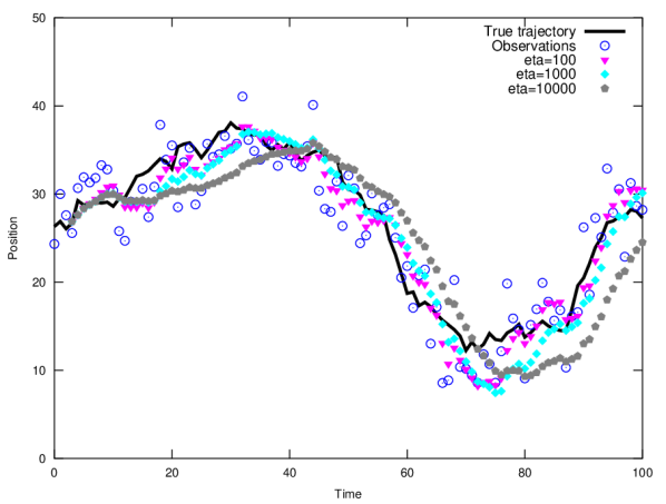
Figure 1 reveals how the implied approximation in the solution (22) results in the position tracking deviating from ideal at the beginning ($t=0$) of the time series. Without the time-reversal trick, this deviation would have occurred at the end ($t=n$); although the deviation is small, it is significant, but if the time-series window is large enough, then there is no significant effect for $t>10$. Optimal smoothing appears occur in the range $10<\eta<100$.

Figure 2 shows how smaller $\eta$ result in large and rapidly switching accelerations, while larger $\eta$ result in much smaller accelerations applied over longer periods.

Figure 3 demonstrates using the same filter as in figure 1 as a sequential state-estimator; the filter is applied only to the observations up to that time. In the this tracking mode the smoothing parameter $\eta$ is seen to act like an inertial damping. For the larger $\eta=10000$ the tracking lags the true trajectory. For smaller $\eta$ values the tracking is better, but note how a sequence of observations with repeated negative bias for $60<t<75$ result in the tracking over-shotting the turn near $t=70$. When the repeated bias ends around $t=75$ the near optimal $\eta=100$ track jumps back to good estimates, while the $\eta=1000$ track turns back smoothly toward the true trajectory.

3.2 Vector filter with uncorrelated observations

If the observations of each component of the $d$-dimensional position are uncorrelated, then filtering can be accomplished very efficiently using a scale filter, which will come in useful later when non-cartesian observations are considered.

When the observations of each component of the $d$-dimensional position are uncorrelated the covariance matrices $C_{i}$ are all diagonal, and it is unnecessary to use the vectorised filter (27), which has been expanded by an outer product with $I_{d}$; instead it is sufficient to solve  (22) seperately for each component. If all the components have proportionally the same variance at each time, then the singular value decomposition only needs to be solved once for all components, that is, one information matrix $\mathcal{I}$ is needed, whose elements are proportional to the variances, and $\mathcal{P}$ becomes a $(n+1)\times{}d$ matrix of observations, so that eq. (22) then solves for all components of $p$ simultaneously.

(a)	(b)

Figure 4: Position tracking for $0\leq{}t\leq{}150$ of the path $(x,y)=10(t-10)/150+(1/3)(1-t)(\sin(t/15),2-t/15).$ Observational errors independent on each component with standard deviation $5$. (a) Final tracking curves for various $\eta$. (b) Sequential position estimates for $\eta=1000$, that is, last state of a shadowing trajectory obtained using all observations up to a given time.

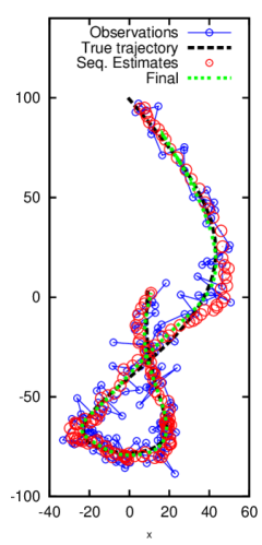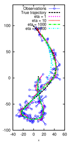
Figure 4 shows tracking in two dimensions in this situation. Observe how a very large $\eta=10000$ results in poor tracking as the tracking curve is pulled toward the mean of the observations. The poor tracking at the beginning can also be observed for larger $\eta$. Fig 4(b) shows the important case of sequential estimates, that is, sequential tracking of the object using all the observations obtained up to a given time. For efficiently reasons, one would in practice only use a finite window of past observations. Details of how to determine the optimal window for a given system and purpose is beyond the scope of this paper and is discussed in the general context of shadowing filters elsewhere [12].

4 Using non-Cartesian observations

A frequently encountered tracking problem involves using bearing and range observations, or combinations of multiple bearing or range observations. Several important situations are worth considering. Active radar location uses range and bearing information. Satellite interferometry uses range and bearing information, but the range is much more accurately measured than the bearing. Global positioning by satellite uses only range information, but from multiple reference satellites. Tracking wireless devices can use range information inferred from signal power at multiple transponders. Passive sonar location provides bearing information, but poor range; often bearings from multiple sensor points are used.

All of the applications mentioned can be dealt with using the vector filter (27), by transforming the observations into raw Cartesian position estimates and computing the appropriate information matrix. The transformations are simple geometry, but computing the information matrices requires some approximation or restrictions.

Let $p\in\mathbb{R}^{d}$ be the position in Cartesian coordinates, and let $q\in\mathbb{R}^{d}$ be a vector of $d$ noise-free observations of the position is some other coordinates. Suppose there is an invertible function $f$, on some domain, such that $p=f(q)$. Given a noisy observation $\mathcal{Q}=q+\Delta q$, the transform $f$ provides a raw position estimate $\mathcal{P}=f(\mathcal{Q})=p+\Delta p$. Given the covariance matrix $C_{q}$ of the observations, the covariance $C_{p}$ of the estimate is required. The column vector $\Delta q$ is the error in the observation, and to a first approximation, the error in the estimate is $\Delta p\approx{}J\Delta q$, where $J=\partial_{q}f(q)$ is the Jacobian matrix of $f$ at $q$. Since the covariance $C_{p}$ is the expected value of the outer product $\Delta p\Delta p^{T}$, it follows that, to a first approximation, $C_{p}=JC_{q}J^{T}$. It also follows that the corresponding information matrices are related by $\mathcal{I}_{p}=K^{T}\mathcal{I}_{q}K$, where $K=J^{-1}=\partial_{p}(f^{-1})$. Note that since only the information matrix is needed in the shadowing filter under discussion, it is sometimes easier to compute the $K$ directly using $f^{-1}$, than it is to compute $J$ and invert it. This is the case in some of the following examples.

An important problem, which will be returned to in each of the following sections, is that although the correlation matrix $C_{q}$ may be well known, the transformation matrices $J$ and $K$ depend on the target’s location, which is unknown. The raw position estimate $\mathcal{P}=f(Q)$ could be used, but this introduces errors in the supposed covariance. When the transformed coordinates are highly correlated and the transform very non-linear, then a small error in the raw position estimate can give rise to a very wrong estimate in the correlation. This problem plagues Kalman filters, and other filters that need a covariance estimate to reliably estimate the state. A significant advantage of a shadowing filter is the robustness gained from finding a shadowing trajectory, rather than just a current position estimate. This robustness means that the correlation in the raw position estimates are of little importance, that is, ignoring the correlation can have little effect on the quality of the tracking.

4.1 Range and bearing observations

Consider a target tracked in the plane, position $p=(x,y)$, using observations $q=(r,\theta)$, where $r$ is the range from a reference point $(a,b)$ and $\theta$ the bearing in radians measured in the anti-clockwise direction from the $x$-axis. The transformation $p=f(q)$ is given by

$$x = a+r\cos\theta,$$ (30)

$$y = b+r\sin\theta.$$ (31)

Under the assumption that $r$ is not close to zero, and the variances of $r$ and $\theta$ are small, then the covariance and information matrix of $x$ and $y$ are approximated as previously described using

$$J=\begin{pmatrix}\cos\theta&-r\sin\theta\\ \sin\theta&r\cos\theta\end{pmatrix}$$ (32)

or

$$K=\begin{pmatrix}\cos\theta&\sin\theta\\ -(1/r)\sin\theta&(1/r)\cos\theta\end{pmatrix}.$$ (33)

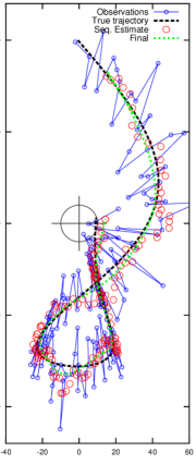
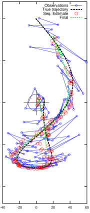
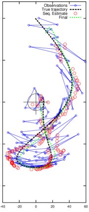
Figure 5 shows the tracking of a target using range and bearing information of different accuracy. In panels (a) and (b) the correlation of the raw position estimates is ignored, and the results are good, that is, the shadowing filter provides significant improvement over the raw position estimates. Panel (c) uses the same data as panel (b), but tries to take into account the correlation of the raw position estimates using the correlation computed at the raw position estimate; the result is worse than assuming no correlation. If the same is attempted for the data of panel (a), the result is a worse failure, because the radius is poorly estimated and since this appears as a reciprocal in the transformation, small errors in the radius can lead to very poorly estimated correlations, so much so that the quality of the filtering is much worse.

This example provides an excellent illustration of how the robustness of a shadowing filter has significant gains over other filters. Not only does ignoring the correlation result is better tracking, it is also more efficient, because rather than using the vectorised filter (27), the simpler, more compact, scalar filter (22) can be used.

(a)	(b)	(c)

Figure 5: Position tracking of same path as fig. 4. Circle with cross-hair is the observation site. Sequential position estimates and final trajectory estimate for $\eta=1000$. (a) Bearing measurement ten times more accurate than range. (b) Range measurement ten times more accurate than bearing. In both (a) and (b) the estimation ignores correlations and treats each component as being independent. (c) As case (b) but using correlation as computed from raw position estimate; this does worse than (b), because the correlation is calculated relative to the raw position estimates, which are very misleading.

4.2 Multiple bearing observations

Consider a target tracked in the plane, position $p=(x,y)$, using bearing observations $q=(\theta,\theta^{\prime})$ from two distinct reference points $(a,b)$ and $(a^{\prime},b^{\prime})$. Under most circumstances there exists unique $s,s^{\prime}\in\mathbb{R}$ such that

$$(x,y) = (a,b)+s(\cos\theta,\sin\theta)$$ (34)

$$= (a^{\prime},b^{\prime})+s^{\prime}(\cos\theta^{\prime},\sin\theta^{\prime}).$$ (35)

Hence, a raw position estimate can be found by solving the linear equations

$$\begin{pmatrix}\cos\theta&-\cos\theta^{\prime}\\ \sin\theta&-\sin\theta^{\prime}\end{pmatrix}\begin{pmatrix}s\\ s^{\prime}\end{pmatrix}=\begin{pmatrix}a^{\prime}-a\\ b^{\prime}-b\end{pmatrix},$$ (36)

provided the equations are consistent and non-singular. Since the angles are observed angles, inconsistency can occur when $\theta^{\prime}\approx\pm\theta$. For some sequential filters such nearly-singular situations can be devastating, but, since the shadowing filter is estimating a trajectory from a sequence of observations, there is generally no harm in simply dropping observations corrupted by near-singularities, or replacing them with forecasted positions, or crudely interpolated positions. There is generally no harm in doing either of these for short periods. Dropping observations requires using a larger $\tau$ time-gap between observations. If the observations were equally spaced in time, this leads to a lot of special computation, and so in this case it is generally easier to insert a forecasted position with a suitably scaled down information matrix to account for the errors in the forecast; see details given later.

In this multiple-bearing situation it is difficult to compute $J$ directly, but $K$ is easily computed. Note that

$$\theta=\arctan\frac{y-b}{x-a}\qquad\text{and}\qquad\theta^{\prime}=\arctan\frac{y-b^{\prime}}{x-a^{\prime}}.$$ (37)

It follows that

$$K=\begin{pmatrix}(x-a)/r^{2}&(y-b)/r^{2}\\ (x-a^{\prime})/r^{\prime 2}&(y-b^{\prime})/r^{\prime 2}\end{pmatrix},$$ (38)

where $r^{2}=(x-a)^{2}+(y-b)^{2}$ and ${r^{\prime}}^{2}=(x-a^{\prime})^{2}+(y-b^{\prime})^{2}$, which requires only trivial computation once an estimate of $(x,y)$ is obtained.

As mentioned, a significant problem arises when the sensors and target are collinear, $\theta\approx\pm\theta^{\prime}$, because the linear equations (36) are singular or badly conditioned. This can result in raw position estimates far their true position. Figure 6 shows an example of tracking using two mobile sensors for detecting bearing, and a mobile target. In this example the target moves on a circular path clockwise from the 12 o’clock position. When the target is between the 4 and 5 o’clock position it is directly between the sensors, and at the end of its path, around the 7 o’clock position, the target is almost directly behind both sensors. Both of these situations lead to a poorly conditioned matrix in eq. (36) and hence poor raw position estimates.

For the estimates shown in fig. 6 the component correlations of the raw position estimate are ignored, as in fig 5(a) and (b). The ill-conditioning is dealt with by using the 1-norm estimate of the reciprocal condition as returned by LAPACK [2]. This number varies between zero and one, with small values indicating bad conditioning. This norm is a natural candidate to scale the information matrices to give raw position estimates from poorly conditioned situations small weight.

Figure 6: Position tracking using bearings from two moving sensors. For $0\leq{t}\leq 100$ one sensor moves between $(-3,3)$ and $(3,1)$, and the other between $(-3,-2)$ and $(3,-1)$, both at constant speed, while the target moves on the circular path $(\sin(t/25),\cos(t/25))$. The centre of the circles is the position of the sequential state estimates, the diameter of the circle indicates the condition-number weight applied to that position’s raw position estimate.

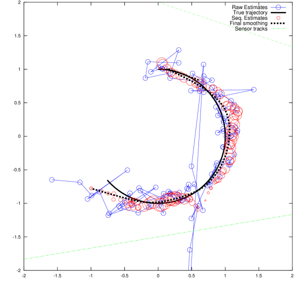
From fig. 6 it can be seen that when the raw position estimates are obtained under good conditioning, the sequential estimates (large circles) are good. Under poor conditioning (small circles) the sequential estimates are mainly forecasts from the preceding trajectory positions, and the wild raw position estimates are ignored. When the target passes beyond the 5 o’clock position and conditioning improves, and the sequential estimates return to good position estimates. Note also that the final trajectory almost exactly matches the true trajectory through the 4 to 5 o’clock position.

4.3 Multiple range observations

Consider a target tracked in the plane, position $p=(x,y)$, using range observations $q=(r,r^{\prime})$ from two distinct reference points $(a,b)$ and $(a^{\prime},b^{\prime})$. Under most circumstances the location can be obtained from the solutions of $r^{2}=(x-a)^{2}+(y-b)^{2}$ and ${r^{\prime}}^{2}=(x-a^{\prime})^{2}+(y-b^{\prime})^{2}$, assuming that the non-uniqueness can be resolved. By taking partial derivatives of these two equations with respect to $x$ and $y$, it follows implicitly that

$$K=\begin{pmatrix}(x-a)/r&(y-b)/r\\ (x-a^{\prime})/r^{\prime}&(y-b^{\prime})/r^{\prime}\end{pmatrix}.$$ (39)

5 Partial observations

Our stated formulation of the tracking problem allows for non-uniformly spaced observations, but all examples thus far have used only uniformly spaced observations. We make a simple demonstration using non-uniformly spaced observations by considering a situation where observations are missing.

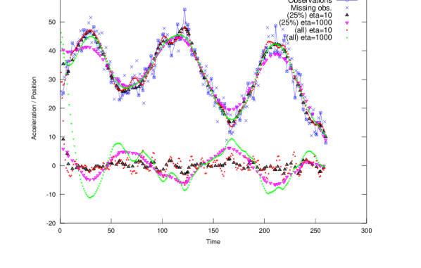
Figure 7 demonstrates tracking using similar data to figure 1 where 75% of the observations are missing, comparing this to the tracking calculations when all observations are available. Two values of the smoothing parameter $\eta$ are used. These results demonstrate that the tracking algorithm is very robust. The position tracking is very similar when there is missing observations. The acceleration estimates are also very similar. Overall the tracking is slightly smoother, and accelerations less variable, when there is missing data, but this is something of an artifact, because the effective amount of smoothing for a fixed $\eta$ depends on the amount of observations available; less data results in more smoothing.

Figure 7: Position tracking and accelerations using similar data to figure 1 and 2, but with partial observations for two $\eta$ smoothing values. The first two curves show calculations when 75% of observations are missing, with crosses marking the missing observations, and the second two curves using all observations.

6 Conclusion

Under the assumption of piecewise constant accelerations a shadowing filter algorithm has been derived and implemented efficiently for scalar time-series of observations. Vector time-series of observations can be dealt with efficiently using the same algorithm if each component is observed with uncorrelated errors.

The scalar algorithm can be easily extended to deal with tracking in $d$-dimensions where the position vector components are not observed directly and a transformation of the observations can be used to obtain an initial raw position estimate. The question then arises of how to deal with the correlation of the errors this introduces. Remarkably, experiments reveal, as illustrated in figs 4, 5 and 6, that ignoring this correlation has little significant effect. Simply using the raw position estimates to estimate the correlations produced worse position estimates, because errors in the raw position estimates give misleading indications about the correlation. This problem is unvoidable to Kalman filters. It may be that some more complex algorithm could be devised to better estimate the correlations, but this will increase the amount of computation, for possibly no significant gain. Just taking correlations into account in the stated algorithm increases the size of matrix requiring singular value decomposition from $n(n+1)$, to $d^{2}n(n+1)$ entries, so the computation cost is significant.

There are a number of other implementation issues that have not been discussed, the most important of which is the optimal window size $n$ for obtaining a shadowing trajectory and position estimates. The window size is problem depended, but a method for determining an appropriate window size is discussed at length elsewhere [12]. This cited work also discusses issues of how best to implement sequential filtering.

References

- [1] B. D. O. Anderson and J. B. Moore. Optimal Filtering. Prentice-Hall, Englewood Cliffs, New Jersey, 1979.
- [2] E. Anderson, Z. Bai, C. Bischof, S. Blackford, J. Demmel, J. Dongarra, J.Du Croz, A. Greenbaum, S. Hammarling, A. McKenney, and D. Sorensen. LAPACK User’s Guide. SIAM, (http://www.netlib.org/lapack/lug/lapack_lug.html), third edition, 1999.
- [3] Y. Bar-Shalom, X. R. Li, and T. Kirubarajan. Estimation with Applications to Tracking and Navigation. John Wiley and Sons, 2001.
- [4] C.H. Davis. Theory Of The Motion Of The Heavenly Bodies Moving About The Sun In Conic Sections: A Translation Of Gauss’s Theoria Motus (1857). Dover, 2004.
- [5] G.D. Forney. The Viterbi algorithm. Proceedings of the IEEE, 61(3):268––278, 1973.
- [6] I. Gilmour. Nonlinear model evaluation: iota-shadowing, probabilistic prediction and weather forecasting. PhD thesis, Mathematical Institute, Oxford University, 1998.
- [7] A. H. Jazwinski. Stochastic Processes and Filtering Theory, volume 64. Academic Press, New York, 1970.
- [8] K. Judd. Forecasting with imperfect models, dynamically constrained inverse problems, and geometrically modified gradient descent. Physica D, 237:216–232, 2008.
- [9] K. Judd and T. Stemler. Failure of sequential Bayesian filters and the advantages of shadowing filters. Physical Review E, 79:066206, 2009.
- [10] R. P.S. Mahler. Statistical Multisource-Multitarget Information Fusion. Artech House, 2007.
- [11] W. H. Press, B. P. Flannery, S. A. Teukolsky, and W. T. Vetterling. Numerical Recipes in C. Cambridge University Press, Cambridge, 1988.
- [12] T. Stemler and K. Judd. A guide to shadowing filters for forecasting and state estimation. Physica D, 238:1260–1273, 2009.