From depinning transition to plastic yielding of amorphous media:
A soft modes perspective

Abstract

A mesoscopic model of amorphous plasticity is discussed in the context of depinning models. After embedding in a $d+1$ dimensional space, where the accumulated plastic strain lives along the additional dimension, the gradual plastic deformation of amorphous media can be regarded as the motion of an elastic manifold in a disordered landscape. While the associated depinning transition leads to scaling properties, the quadrupolar Eshelby interactions at play in amorphous plasticity induce specific additional features like shear-banding and weak ergodicity break-down. The latters are shown to be controlled by the existence of soft modes of the elastic interaction, the consequence of which is discussed in the context of depinning.

I Introduction

Most liquids flow as soon as they experience shear stress. In contrast many complex fluids (pastes, foams, colloidal suspensions, etc.) do not flow for shear stresses lower than some threshold yield limit. The rheological behavior of these yield-stress fluids parallels the plasticity of amorphous solids (oxide and metallic glasses, polymers, etc.). Both families of materials exhibit a rich phenomenology. Close to the yielding threshold, critical-like behaviors are observed: avalanches Sun et al. (2010); Antonaglia et al. (2014), growth of a correlation length scale Goyon et al. (2008), Hershell-Bulkley law Coussot (2014)… In parallel other properties are reminiscent of glassy phenomena: e.g. thermal Cheng et al. (2008) and mechanical Perriot et al. (2006); *VDCPBCM-JPCM08; Dmowski and Egami (2008); Révész et al. (2008) history dependence. In the same spirit, strain localization Lewandowski and Greer (2006); Divoux et al. (2011), a phenomenon of crucial technological interest (since it controls the mechanical strength) can be analyzed as an ergodicity break-down process: plastic activity is trapped in a very limited sub-region of the phase space Török et al. (2000).

These two phenomenological archetypes (criticality and glass transition) have motivated parallel modeling efforts. Building on trap models Bouchaud (1992) designed to capture ergodicity breaking and aging at glass transition, Sollich et al. Sollich et al. (1997); *Sollich-PRE98; Fielding et al. (2009); *Fielding-PRL11 developed Soft Glassy Rheology (SGR) models and could associate different rheological behaviors of complex fluids to a parameter of their model, an effective temperature associated to mechanical noise (see a recent discussion in Nicolas et al. (2014a)). A different glassy approach has been pursued by Bouchbinder and LangerBouchbinder and Langer (2009a); *Bouchbinder-PRE09b; *Bouchbinder-PRE09c who extended the Shear-Transformation-Zone theoryFalk and Langer (1998) to explicitly account for an effective temperature related to the slow configurational degrees of freedom of the glassy material under shear.

The need to go beyond mean field description and understand the crucial effect of elastic interactions associated to the localized rearrangements (Eshelby events) Spaepen (1977); Argon (1979); Falk and Langer (1998); Maloney and Lemaître (2004a); Tanguy et al. (2006) responsible of amorphous plasticity has early led to the development of mesoscopic models accounting for these interactions Bulatov and Argon (1994a); *BulatovArgon94b; *BulatovArgon94c. This effort of modeling amorphous plasticity and/or rheology of complex fluids at mesoscopic scale has, since then, been very active Baret et al. (2002); Talamali et al. (2011); *TPVR-Meso12; Picard et al. (2002); *Picard-PRE05; Lemaître and Caroli (2006); Jagla (2007); Dahmen et al. (2009); Homer et al. (2010); Martens et al. (2011); Budrikis and Zapperi (2013); Homer (2014); Nicolas et al. (2014b); Lin et al. (2014a, b). As early noticed in Baret et al. (2002), the competition at play in mesoscopic models between microscopic disorder and elastic interaction strongly reminds the physics of the depinning transition Fisher (1998); *Kardar-PR98 that naturally entails critical features. Recently summarized in Ref. Lin et al. (2014b), most features of the associated scaling phenomenology predicted by depinning-like models of amorphous plasticity have been observed numerically Maloney and Lemaître (2004b); Demkowicz and Argon (2005); Maloney and Robbins (2008); *Maloney-PRL09; Salerno et al. (2012); *Salerno-PRE13 and experimentally Sun et al. (2010); Antonaglia et al. (2014).

Noteworthily, some of the key non-ergodic features (e.g. aging and shear-bandingVandembroucq and Roux (2011); *BV-AIP13; Martens et al. (2012); Homer (2014)) can be also recovered within the framework of the mesoscopic elastoplastic models. This has raised the question of the precise link with the depinning transition. In particular, the crucial effect of the non-positiveness of the quadrupolar elastic interaction induced by individual plastic events has been questioned. Recently Lin et al. Lin et al. (2014b) have shown the necessity of three independent exponents (instead of two for standard depinning) to account for the scaling properties of mesoscopic models of amorphous plasticity.

Here we show that the specific features observed in elasto-plastic models are controlled by the presence of multiple soft modes of the quadrupolar elastic interaction. Note that the presence of such soft modes is not an artifact of lattice discretization or of a specific numerical implementation Budrikis and Zapperi (2013). In the present perspective, shear bands directly result of the Eshelby interaction symmetry i.e. extended modes of plastic deformation that satisfy compatibility and consequently induce no internal stress. This property, absent in classical depinning models, has dramatic effects on the stability, the dependence on initial conditions as well as the ergodicity properties of plastic yielding models.

In the following we present in section I the details of the mesoscopic models of amorphous plasticity. We give a particular emphasis on the comparison with the models of depinning an elastic manifold in a random landscape. The emergence of anisotropic elastic interactions associated to local plastic inclusions is discussed. In section III, a comparison is presented between numerical results on strain fluctuations obtained with Mean-Field (MF) and “Eshelby” anisotropic elastic kernelsEshelby (1957); Picard et al. (2004). In section IV, a Fourier space analysis allows us to unveil the presence of multiple soft modes of the Eshelby elastic interactions. We show in section V that this soft mode analysis sheds a new light on the diffusion and shear-banding behaviors of the mesoscopic models of amorphous plasticity. Our main results are finally summarized in section VI.

II Depinning-like models for amorphous plasticity

II.1 A scalar mesoscopic model

Here we restrict ourselves to a simple scalar case Talamali et al. (2012). Assuming, bi-axial loading conditions, we define respectively for stress and strain the scalar quantities $\sigma=\sigma_{yy}-\sigma_{xx}$, $\varepsilon=\varepsilon_{yy}-\varepsilon_{xx}$ from their tensor counterparts. The material is discretized on lattice at a mesoscopic scale $\ell$ and is assumed to be elastically homogeneous. A simple plastic criterion is defined from the comparison between the local values of the scalar equivalent stress field $\sigma(\mathbf{r},\{\varepsilon^{pl}\})=\sigma^{ext}+\sigma^{int}[\mathbf{r},\{\varepsilon^{pl}\}]$ with a threshold stress $\sigma^{c}[\mathbf{r},\varepsilon^{pl}(\mathbf{r})]$. The local stress $\sigma$ results from the addition of a spatially uniform external stress $\sigma^{ext}$ and of a spatially fluctuating internal stress $\sigma^{int}$ due to the successive plastic rearrangements mediated by the elastic interactions. Here the local stress threshold $\sigma^{c}$ encodes the disordered nature of the structure, it depends both on space and on the local value of the plastic strain $\varepsilon^{pl}$.

From this local criterion a simple equation can be written to model the evolution of the plastic strain field:

$$\partial_{t}\varepsilon^{pl}(\mathbf{r},t)=\mathop{\mathcal{P}}\left(\sigma^{ext}\!+G^{el}\!*\!\varepsilon^{pl}(\mathbf{r},t)\!-\!\sigma^{c}[(\mathbf{r},\varepsilon^{pl}(\mathbf{r},t)]\right)$$ (1)

Here the threshold dynamics is accounted for by the positive part function $\mathop{\mathcal{P}}(\cdot)$ such that $\mathop{\mathcal{P}}(x)=x$ if $x>0$ and $\mathop{\mathcal{P}}(x)=0$ if not.

The heterogeneity of the plastic yield stress at mesocopic scale is represented by the quenched variable $\sigma^{c}$. The latter is defined by its average $\langle\sigma^{c}\rangle=\overline{\sigma^{c}}$ and its correlations $\langle\sigma^{c}(\mathbf{r},z)\sigma^{c}(\mathbf{r}+\mathbf{\delta r},\varepsilon^{pl}+\delta\varepsilon^{pl})\rangle=\varsigma^{2}f(\mathbf{\delta r})g(\delta\varepsilon^{pl})$ where $\varsigma^{2}$ gives the variance. Short-range correlations are considered, namely, $f(\mathbf{\delta r})\to 0$ if $|\mathbf{\delta r}|\gg\ell$ and $g(\delta z)\to 0$ if $|\delta\varepsilon^{pl}|\gg e_{0}$. The length scale $\ell$ is given by the mesoscopic scale at which coarse-graining is performed. The strain scale $e_{0}$ corresponds to the typical plastic strain induced by elementary plastic events.

Finally the internal stress $\sigma^{int}$ is represented through a convolution of the plastic strain field $\varepsilon^{pl}$ and the elastic kernel $G^{el}$ associated with the reaction of the matrix to a unit local plastic strain: $\sigma^{int}=G^{el}*\varepsilon^{pl}$ (Eshelby inclusion Eshelby (1957)). The properties of this long-ranged and anisotropic elastic interaction are discussed in more details in sub-section II.3

Instead of directly integrating Eq. (1), an extremal dynamics algorithm of the model discretized on a lattice is implemented Baret et al. (2002). Only one site (the weakest one) experiences plastic deformation at each iteration step. The external stress is adjusted accordingly. Such an algorithm corresponds to shearing the system at a vanishing strain rate and is very close in spirit to the athermal quasi-static protocols under conditions of imposed strain developed in atomistic simulationsMaloney and Lemaître (2004b, 2006).

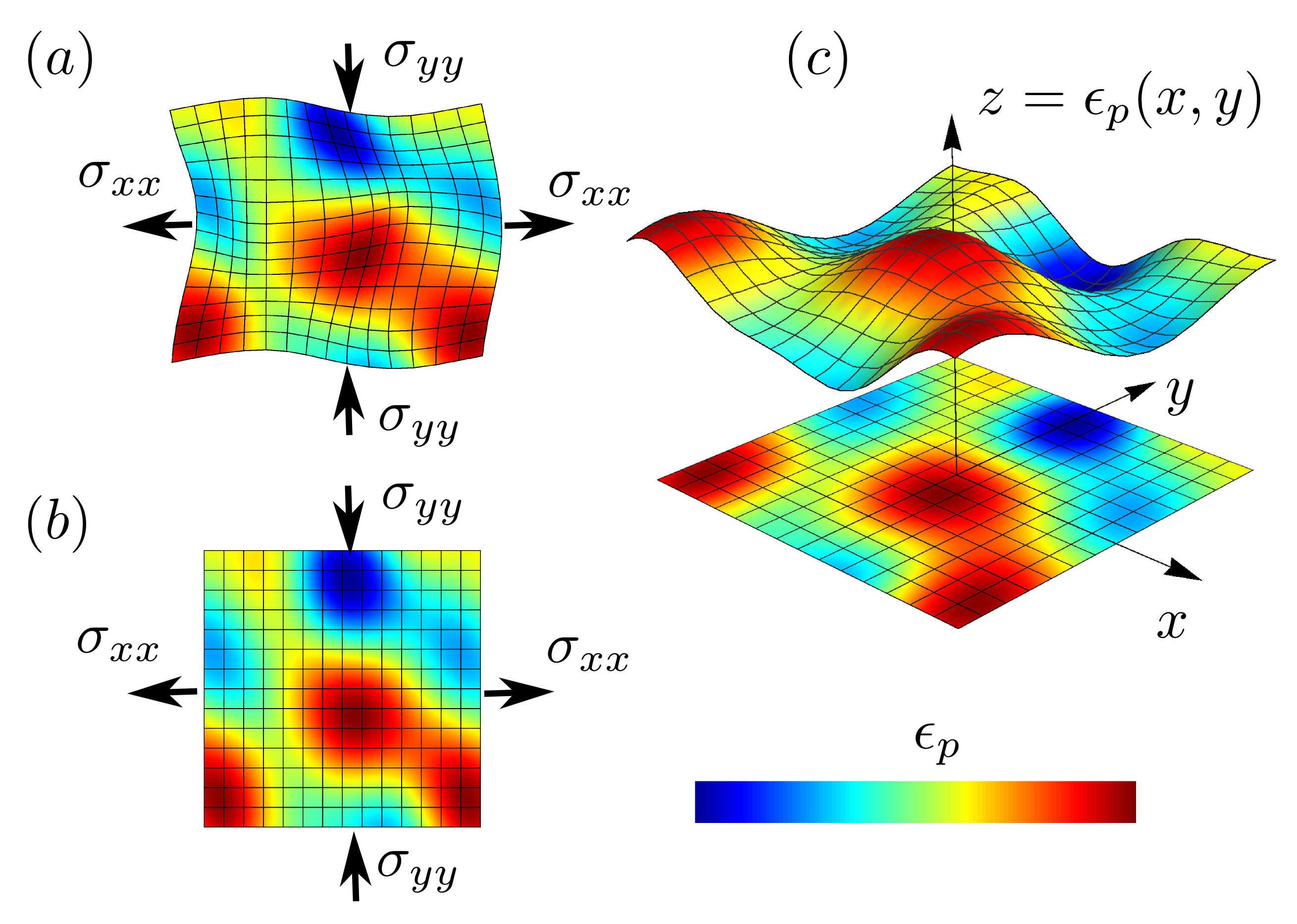
Figure 1: Sketch of a 2d amorphous material upon bi-axial loading. (a) The mesh is deformed according to the displacement. The associated strain has a reversible elastic contribution and an irreversible plastic contribution. The latter is represented according to the color scale. (b) The plastic strain field (colors) is represented on the un-deformed reference frame. (c) The plastic strain field can be represented as a $d$-dimensional manifold moving in a $d+1$ space.

II.2 From plastic yielding to depinning

In the framework of upscaling amorphous plasticity from the microscopic to the macroscopic scales Rodney et al. (2011), the equation of evolution (1) can be understood in one of the two ways. First it can be seen as presented above i.e. as a description of the (visco-)plastic dynamics of a plastically heterogeneous material, discretized at scale $\ell$.

Second, such a threshold dynamics also naturally emerges after coarse-graining (in the direction of motion) from the equation of evolution of a driven elastic manifold in a continuous random landscape. In order to illustrate this direct mapping to depinning we discuss in the following the geometry of the equivalent manifold and the emergence of the threshold dynamics associated to the multistability of the elastic interface.

Let us recall the equation of evolution of the overdamped motion of an elastic manifold $h({\mathbf{x}})$ in a random landscape Fisher (1998); *Kardar-PR98:

$$\partial_{t}h(\mathbf{r},t)=f^{ext}(t)+G^{el}\!*\!h(\mathbf{r},t)-\frac{\partial U}{\partial h}\left[\mathbf{r},h(\mathbf{r},t)\right]$$ (2)

Here $f^{ext}$ stands for the external driving force, $G^{el}*h$ for the elastic restoration force and $U$ is a random potential such that $\langle\partial_{\mathbf{r}}U\rangle=0$ and $\langle\partial_{\mathbf{r}}U(\mathbf{r},z)\partial_{\mathbf{r}}U(\mathbf{r^{\prime}},z^{\prime})\rangle=\varsigma^{2}f(\delta r/\ell)g(\delta z/e_{0})$ where $\ell$ and $e_{0}$ give the correlation lengths along the manifold and in the direction of propagation, respectively.

The present depinning equation is very close to Eq. (1) proposed to model amorphous plasticity. In the latter the external stress plays the role of the driving force for the depinning, the elastic kernel associated to the Eshelby inclusions corresponds to the elastic restoration force and the disordered stress thresholds are associated to the random potential.

To illustrate more clearly the direct analogy between deformation under shear and motion of an elastic manifold we give here a simple geometric interpretation. Let us consider the plastic strain field $\varepsilon_{p}(\mathbf{r})$ of a $d$-dimensional material. As sketched on Fig. 1, we can define an extra coordinate $z$, orthogonal to the space variable $\mathbf{r}$ after embedding in a $d+1$ dimensional space. The equation $z=\varepsilon^{pl}(\mathbf{r})$ thus defines an elastic manifold whose propagation in the random landscape $\sigma^{c}[\mathbf{r},\varepsilon^{pl}(\mathbf{r},t)]$ is governed by Eq. (1).

An obvious difference still remains between the two equations. While the the depinning equation (2) models a continuous evolution, the equation (1) shows a discontinuous threshold dynamics, here encoded by the presence of the $\mathop{\mathcal{P}}(.)$ function. We argue here that, far from being different in nature, such a threshold dynamics is a direct outcome of the competition between elasticity and disorder upon coarse-graining in the direction of propagation..

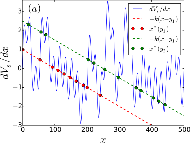
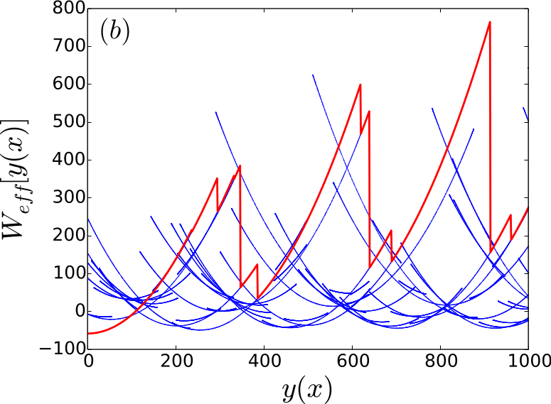
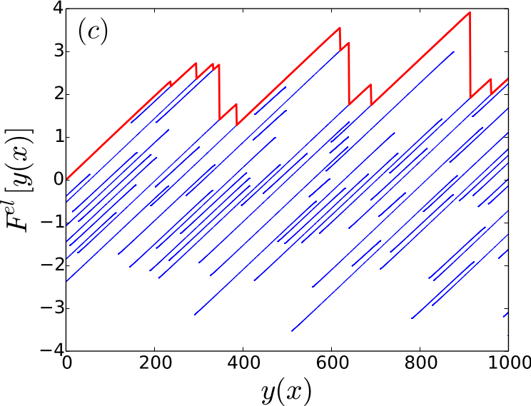
Figure 2: Phenomenology of the motion of a particle of position $x$ driven by a spring of position $y$ in a one-dimensional random potential $V(x)$: (a) Graphical representation of the multiplicity of the solutions of the equilibrium equation $V^{\prime}(x)=-k(x-y)$ for two positions of the spring. (b) Parametric represntation of the complex effective potential $W_{eff}(y)$ seen by the spring and representaion (in red) of on eparticular trajectory. (c) Associated represntation of the force landscape. Jumps in the potential $W_{eff}$ are associated to force thresholds.

In order to give more support to the latter statement we resort in the following to a simple example early developed in the close contexts of solid friction Caroli and Nozières (1998); *Tanguy-PRE97; *Baumberger-AdvPhys06 and rate independent plasticity Puglisi and Truskinovsky (2005), the over-damped dynamics of an isolated point driven into a one-dimensional random potential:

$${\partial_{t}}x =-{\partial_{x}}\left[\frac{k}{2}\left(x-y\right)^{2}\right]-V^{\prime}(x)$$

$$=-{\partial_{x}}W(x,y)$$

where $V$ is a random potential such that $\langle V^{\prime}(x)V^{\prime}(x^{\prime})\rangle=\varsigma^{2}f[(x-x^{\prime})/e_{0}]$ where $f(u)\to 0$ for $|u|\ll 1$. Here $y$ denotes the external driving (e.g. at finite velocity $y=vt$) and $k$ is the strength of the confining potential (the stiffness of the spring driving the system).

Such a system of total energy $W(x,y)=k(x-y)^{2}/2+V(x)$ is known to exhibit multistability when disorder overcomes elasticity. Namely if $k\varsigma/e_{0}>1$, for every $y$ position, one and only one position $x^{*}(y)$ satisfies equilibrium and stability conditions: $\partial_{x}W(x,y)=0$ and $\partial^{2}_{xx}W(x,y)>0$. An effective potential $W_{\mathrm{eff}}(y)=W[x^{*}(y)]$ can then be defined unambiguously.

Conversely, as illustrated in Fig. 2a that shows graphical solutions of the equilibrium equation $-k(x-y)=V^{\prime}(x)$, for $k\varsigma/e_{0}<1$ the potential $W$ is characterized by a large number of local minima and several stable positions $x^{*}(y)$ of local equilibrium can be found for a given position $y$.

Still, it is possible in this multistability case to resort to a parametric representation and to build an effective potential $W_{\mathrm{eff}}[y^{*}(x)]=W[x,y^{*}(x)]$ associated to the multiple minima. As shown in Fig. 2b, the stable branches of this effective potential consist of series of truncated parabolas. Upon driving, the system jumps from one local minimum $i$ to another one $j$ as soon as a force exceeds the threshold value $f_{i}=-V(x^{M}_{i})$ associated to the upper bound $x^{M}_{i}$ of the basin of attraction of the minimum $i$ (the intersection with the next parabola). One obviously recovers here the phenomenology of the instability inducing local rearrangements at the atomic scale in amorphous plasticity Maloney and Lemaître (2006).

An example of such an (history-dependent) trajectory made of series of micro-instabilities is shown in Fig. 2b and 2c. A threshold dynamics thus directly emerges from this simple case of an isolated defect. In particular, as shown in Fig. 2c it is clear that upon coarse-graining at scale $\xi$, the dynamics of jumps between basins is entirely controled by the series of threshold forces $f_{i}$.

The phenomenology remains unchanged when dealing with more complex objects like manifolds. Rather than the stiffness of an external device, the disorder has in this case to be compared with the internal elasticity of the manifold. See e.g. Ref. Patinet et al. (2013) for a recent discussion in the context of crack front propagation. Note that the non-regularity of the effective potential induced by multistability is likely to be related to the emergence of a cusp in the correlator of depinning forces observed under renormalization Rosso et al. (2007).

The present model of amorphous plasticity this appears to belong to the wider class of depinning models. We discuss in the next section to what extent the peculiar nature of the Eshelby elastic interaction associated with plasticity does affect the phenomenology of depinning.

II.3 A peculiar elastic interaction

The occurrence of a plastic local rearrangement in the amorphous structure inuces internal stresses due to the reaction of the elastic surrounding matrix. This results in a stress relaxation of the region that rearranged and in an anisotropic long-ranged stress field in the outer matrix. This elastic interaction is very peculiar. In particular, it is non strictly positive: the sign depends on the direction. The elastic interaction thus either favors or unfavors the occurence of future plastic events depending on their position.

The exact internal stress field obviously depends on the details of the rearrangement of the amorphous structure. A classical approximation consists in resorting to a continuum mechanics analysis and in using the solution of the stress induced by a plastic inclusion early proposed by Eshelby Eshelby (1957). More precisely, independently on the precise shape of the inclusion, only the dominant contribution of the internal stress in the far-field is considered.

In the plane strain geometry considered in Fig. 3a, a pure shear plastic inclusion induces a long-range internal stress characterized by a quadrupolar symmetry. In an infinite medium, the dominant term in the far-field and the mean stress drop in the inclusion can be written respectively:

$$G_{Q}(\mathbf{r})=-2\mu^{*}a^{2}\varepsilon_{p}\frac{\cos(4\theta)}{r^{2}}\;,\quad G_{Q}(\mathbf{0})=-\mu^{*}\varepsilon_{p}\;.$$ (4)

where $\mu^{*}$ is an effective elastic modulus, $a$ the mean radius of the inclusion and $\varepsilon_{p}$ the mean plastic strain experienced by the inclusion. Here the subscript Q refers to the quadrupolar symmetry. Note that the amplitude of this quadrupolar elastic interaction is controlled by the product of the “volume” of the inclusion by the mean plastic strain.

For the numerical implementation, bi-periodic boundary conditions are considered and following Ref. Talamali et al. (2012), a quadrupolar lattice Green function is defined from the following expression in the Fourier space:

$$\widetilde{G_{Q}}(p,q)=-A\left[\cos(4\theta_{pq})+1\right]\;,\quad\widetilde{G_{Q}}(0,0)=0\;.$$ (5)

where $\theta_{pq}$ is the polar angle and $(p,q)$ the wavevector in Fourier space. While the first term directly stems from the quadrupolar symmetry of the Eshelby far field expression (4), the null value of the zero frequency term $\widetilde{G_{Q}}(0,0)$ is required by a stationarity condition : a spatially uniform plastic strain induces no internal stress. In other words, no plastic incompatibilities are generated because of the assumption of uniform elastic moduli. When translated to discrete form, it means that $\sum_{i,j}G_{Q}(i,j)=0$, henceforth this condition directly imposes the value of the latice Green function at the origin, i.e. the stress drop:

$$G_{Q}(0,0) = -\sum_{(i,j)\neq(0,0)}G_{Q}(i,j)$$

$$= -\frac{A}{N^{2}}\sum_{(p,q)\neq(0,0)}\left[\cos(4\theta_{pq})+1\right]$$

The prefactor $A$ has the dimension of an elastic modulus. Here it is chosen so that the local stress relaxation in the site that experienced a unit plastic deformation is unity: $G_{Q}(0,0)=-1$.

In the plane shear strain geometry (invariant along the $z$-coordinate) illustrated in Fig. 3a, the quadrupolar elastic interaction $G_{Q}$ is positive in the directions at $\pm\pi/4$ and negative in the directions at $0$ and $\pi/2$. The associated plastic strain field is thus orientated along the diagonals of the $x,y$ plane.

For the sake of completeness, we also illustrate in Fig. 3b another loading geometry: the antiplane shear geometry. Here the strain field is again invariant along the $z$-axis but the system is sheared along the $yz$ direction so that only $u_{z}$ the $z$-component of the displacement field is non zero and the strain component of interest is $\varepsilon_{yz}(x,y)=\partial_{y}u_{z}(x,y)$. Within this antiplane geometry early studied in Ref. Baret et al. (2002), the elastic interaction associated to a plastic inclusion obeys a dipolar geometry: $G_{D}(\mathbf{r})=A\cos(2\theta)/r^{2}$ so that the plastic strain field is orientated along the $x$ direction. The specificity of this loading geometry will be further discussed in section VI.

Due to their long range character, it may be tempting to approximate the “Eshelby” elastic interaction by a simple Mean-Field (MF) interaction Dahmen et al. (2009): $G_{MF}(\bm{r}_{ij})=1/(N^{2}-1)$ if $|\bm{r}|\neq 0$ and $G_{MF}(\bm{0})=-1$. The latter will be used (all other parameters being kept constant) to illustrate the expected behavior of a standard reference depinning model. In the following, we compare the respective effects of Mean-Field and quadrupolar interactions on some specific properties of amorphous plasticity, i.e. strain diffusion and localization. In order to to investigate the origin of the specific effects of the “Eshelby” elastic kernel, we also define a weighted average of two propagators: $G_{a}=(1-a)G_{Q}+aG_{MF}$ where the parameter $a$ gives the relative weight of the mean field. For moderate values of $a$, the quadrupolar symmetry is mainly preserved in the sense that the Green function remains strictly negative in the $0$ and $\pi/2$ directions.

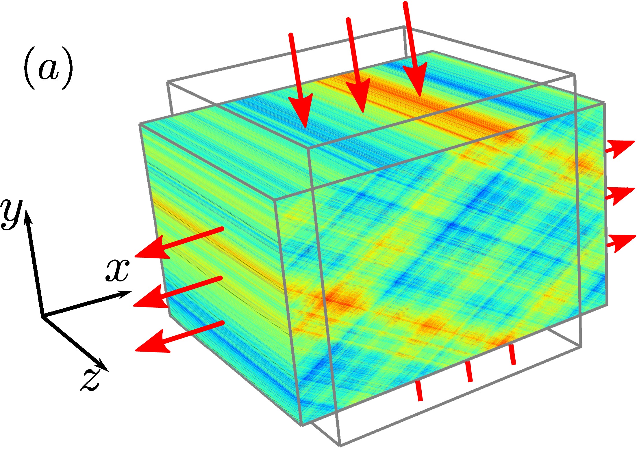
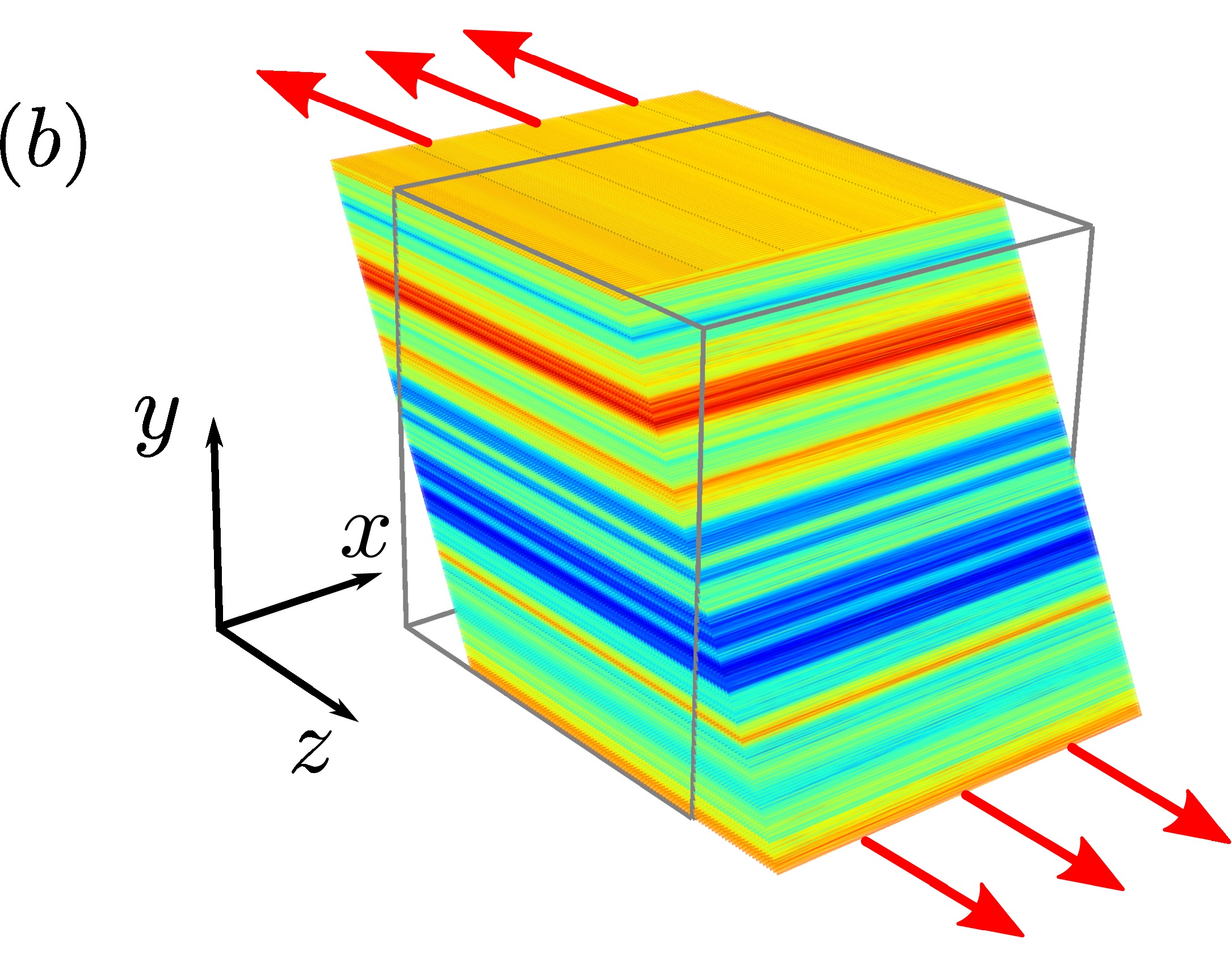
Figure 3: Sketch of two kinds of shear geometry: (a) Plane shear geometry; (b) Antiplane shear geometry. In both cases the strain field is invariant along the $z$-axis. The color scale gives the amplitude in the $xy$ plane of the plastic strain fields (a): $\varepsilon^{pl}=\varepsilon^{pl}_{yy}-\varepsilon^{pl}_{xx}$ and (b) $\varepsilon^{pl}_{yz}$. A quadrupolar symmetry is observed in the plane shear case (a) while a dipolar symmetry is observed in antiplane shear case (b).

III Mean-Field Depinning vs plasticity

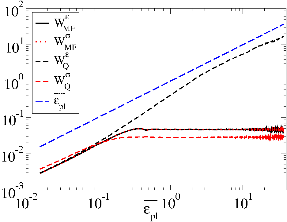
Figure 4: Plastic train variance $W^{\varepsilon}$ and elastic stress variance $W^{\sigma}$ vs cumulated plastic strain $\overline{\varepsilon^{pl}}$ for a quadrupolar propagator $G_{Q}$ and a Mean-Field $G_{MF}$. A linear behavior is represented for comparison.

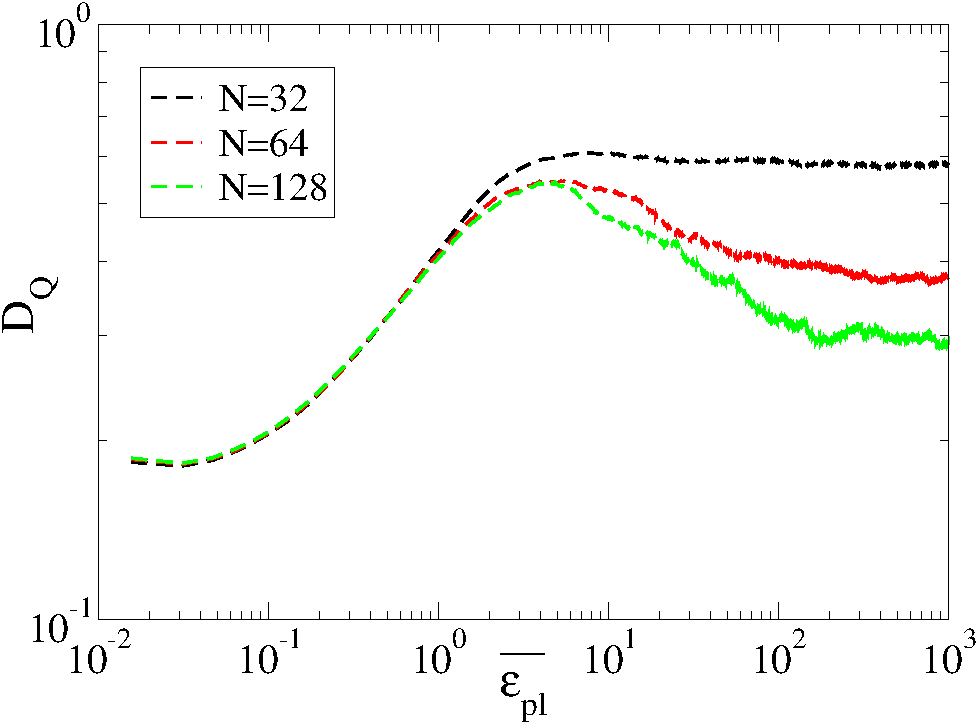
Figure 5: Size-dependent behavior of the plastic strain diffusivity $D_{Q}=W_{Q}^{\varepsilon}/\overline{\varepsilon^{pl}}$ obtained with the quadrupolar kernel $G_{Q}$ for sizes $N=32,\;64,\;128$ with $M=1000,\;100,\;30$ realizations respectively. The larger the system, the longer the anomalous sub-diffusive behavior.

III.1 Family-Vicsek scaling vs Diffusion

We first discuss the behavior of the variance of the plastic strain $W^{\varepsilon}=\langle\overline{|\delta\varepsilon^{pl}|^{2}}\rangle$ where we defined the spatial fluctuation of the plastic strain field $\delta\varepsilon^{pl}=\varepsilon^{pl}-\overline{\varepsilon^{pl}}$). Here $\overline{X}$ and $\langle X\rangle$ denote the spatial average and the ensemble average of the variable $X$, respectively. We show in Fig. 4 (a) the evolution of the variance $W^{\varepsilon}$ with respect to the mean plastic strain $\overline{\varepsilon^{pl}}$. In the context of depinning, as illustrated in Fig 1, $W^{\varepsilon}$ is nothing but the width of the propagating interface. Moreover, in the framework of extremal dynamics used here, the mean plastic strain $\overline{\varepsilon^{pl}}$ defines a fictive time directly associated to the total number of iterations. It is thus legitimate to discuss our results in the framework of the classical Family-Vicsek scaling Narayan and Fisher (1993); Tanguy et al. (1998); Narayan (2000) for interface growth. The latter predicts first for the interface width $W$, a power law growth $W\propto t^{\alpha}$ up to a time scale $\tau\propto L^{z}$ such that the correlation length $\xi$ has reached the system size $\xi(\tau)\approx L$ and beyond which saturation is obtained.

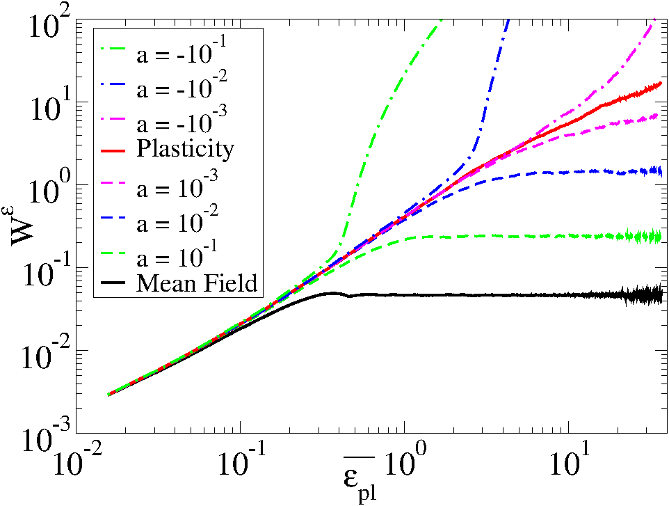
Figure 6: Strain variance (equivalently interface width) vs cumulated plastic strain $\overline{\varepsilon_{pl}}$ for 8 different propagators: $G_{Q}$, $G_{a}$ ($a=\pm 10^{-1},\pm 10^{-2},\pm 10^{-3}$), $G_{MF}$.

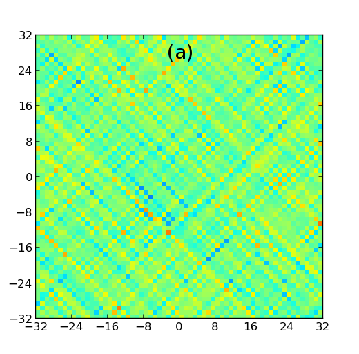
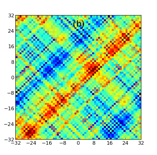
Figure 7: Maps of plastic strain field obtained for a mere quadrupolar elastic interaction (b), and with a positive (a) and a negative (c) MF contribution $a=\pm 10^{-2}$ for $\overline{\varepsilon_{pl}}\approx 5$, past the transient regime. The same color scale has been used in the three cases.

Our numerical results are shown in Fig. 4 for Mean-Field and quadrupolar elastic interactions. As expected, the classical Family-Vicsek scaling is recovered for the width $W_{MF}^{\varepsilon}$ obtained in the case of the Mean-Field depinning. In the amorphous plasticity case, the first power-law growth regime is recovered but, past $\xi\approx L$, the interface width $W_{Q}^{\varepsilon}$ shows no saturation but rather a diffusive trend Talamali et al. (2012). The evolution of the variance $W^{\sigma}$ of the elastic stress field $\sigma^{el}$ is also shown in the two cases. Here saturation is recovered in plasticity as well as in MF depinning. Note that the elastic stress field can be directly obtained from the plastic strain field from a simple convolution with the propagator: $\sigma^{el}=G*\varepsilon^{pl}$. The fact that the diffusive trend at play with the strain field does not show in the stress fluctuations is a first indication that strain fluctuations are controlled by soft modes of the elastic interaction.

In order to characterize in more details the diffusive-like behavior of the plastic strain field obtained with the quadrupolar elastic interaction, we show in Fig. 4(b) the evolution of the associated effective difusivity $D_{Q}=W_{Q}^{\varepsilon}/\overline{\varepsilon_{pl}}$. This ratio is expected to be constant for standard diffusion. At very short times, a plateau is observed; In this very early regime, plastic activity is not correlated yet. Then the diffusivity $D_{Q}$ shows a power-law growth. This simply derives from the fact that in this regime the growth exponent $\alpha$ is larger than unity: $D_{Q}=W_{Q}^{\varepsilon}/\overline{\varepsilon_{pl}}\propto|\overline{\varepsilon_{pl}}|^{\alpha-1}$.

The evolution of the diffusivity then shows a strong size-dependence. For small system size, a simple plateau is obtained, the diffusivity saturates to a constant value. However for larger system sizes a long decreasing transient is observed before a stationary value is obtained. The larger the system, the longer the transient sub-diffusive regime.

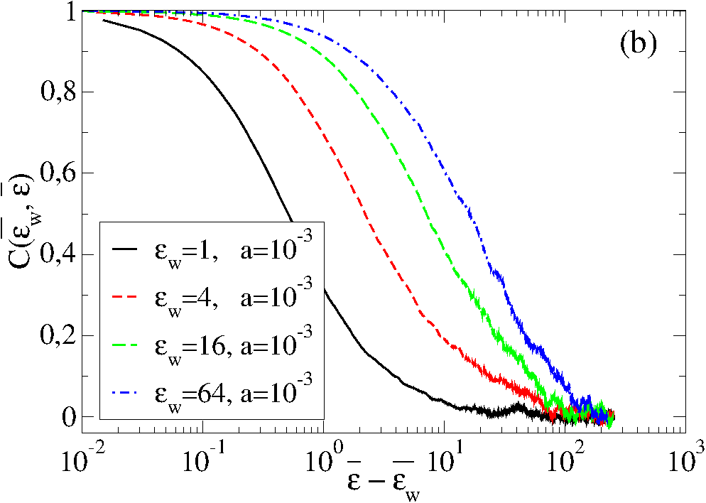
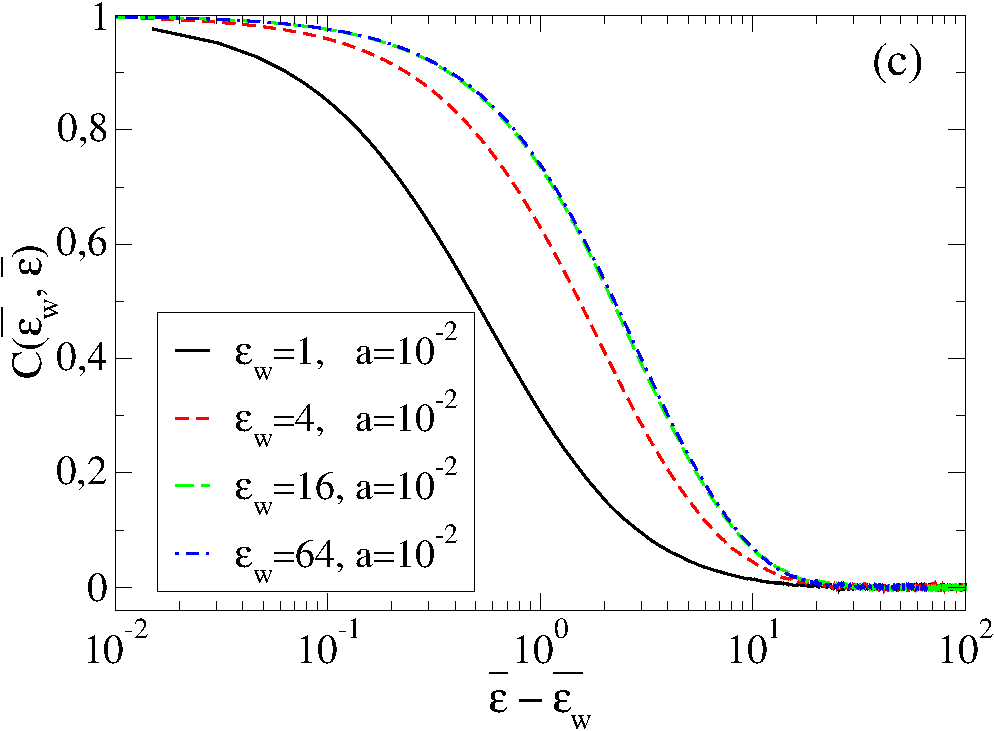
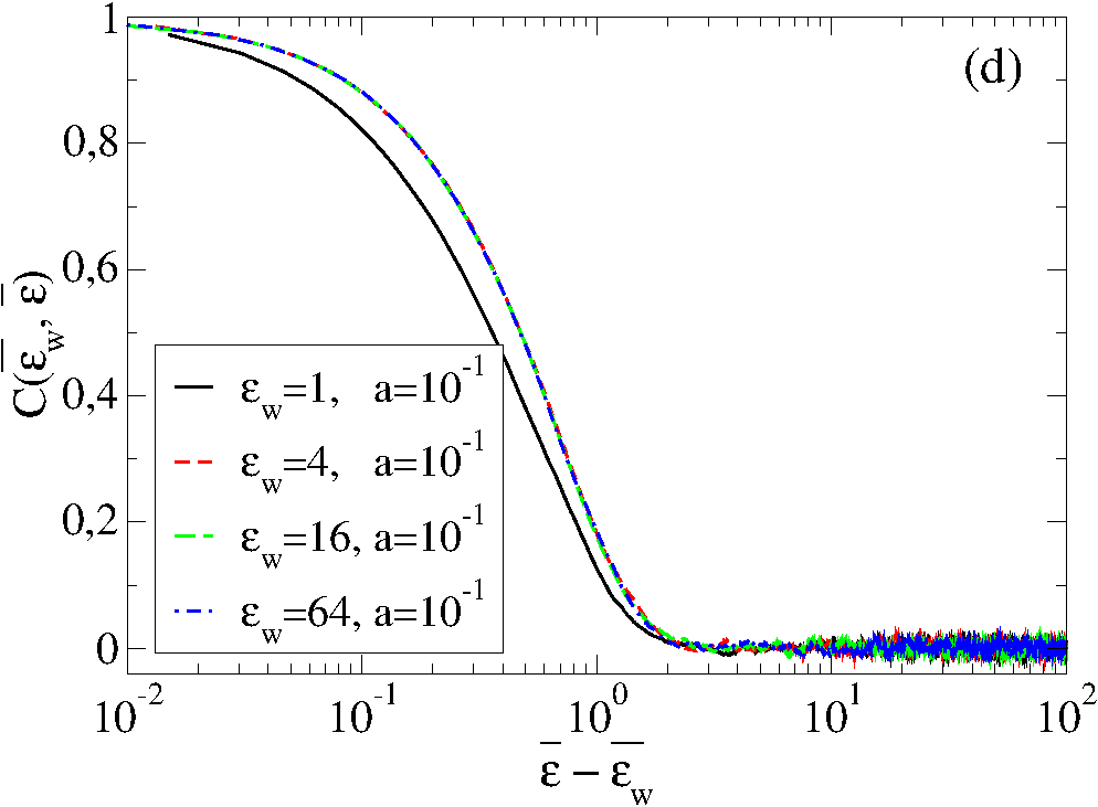
Figure 8: Two-point correlation $C(\overline{\varepsilon_{w}},\overline{\varepsilon})$ of the plastic strain field as a function of the cumulated mean plastic strain $\overline{\varepsilon}$ for 4 “waiting times” $\overline{\varepsilon_{w}}=1,\;4,\;16,\;64$ and for 4 different propagators: $G_{Q}$ (a), $G_{a}$ with a Mean-Field weight $a=10^{-3}$ (b), $a=10^{-2}$ (c) and $a=10^{-3}$ (d). A clear aging effect shows for the quadrupolar propagator $G_{Q}$: the longer the waiting time, the slower the decorrelation. The small MF contributions in propagators $G_{a}$ gradually kills the aging behavior.

III.2 Shear-banding and plastic aging

The nature of the elastic interaction thus strongly affects the evolution of the spatial fluctuations of the plastic strain field and in particular the existence of a diffusive regime. In order to get more insight on the respective effects of the Mean-Field and the quadrupolar kernels, we now show results obtained with the mixed kernel $G_{a}=(1-a)G_{Q}+aG_{MF}$.

In Fig. 7 (top) the evolution of the interface width is shown for different (small) values of $a$. It turns out that even the lowest positive MF contribution is enough to recover saturation at long times. A transient diffusive regime appears when $a$ tends to zero, and the level of the final plateau increases accordingly. But when the interface gets too distorted, if $a>0$ the (low) MF restoring force eventually stops the divergence of the strain fluctuations.

A negative MF contribution $a<0$ has the opposite effect: after a transient diffusive regime, the plastic strain becomes unstable and its variance diverges very fast. The diffusive regime thus appears to be a specific feature of the quadrupolar kernel. It lives on the verge of stability and any mean-field contribution to the elastic kernel sends the system either toward saturation or ballistic evolution depending on the sign of $a$.

The strong effect of the MF contribution is also manifest in the spatial distribution of the plastic strain field. In Fig. 7 (bottom) maps of the plastic strain are shown for a cumulated plastic strain $\langle\varepsilon^{pl}\rangle\approx 5$ for $a=-0.01,\;0,\;0.01$ using the same color scale. The plastic case ($a=0.0$) shows a superposition of patterns localized at $\pm\pi/4$ following the symmetry of the quadrupolar kernel. Similar patterns survive with a positive MF contribution ($a=0.01$) but get very attenuated (the interface width is much lower). A negative MF contribution induces conversely a strong localization behavior: plastic activity is restricted along a unique very thin shear band.

As above mentioned, shear-banding can be analyzed as a kind of ergodicity breakdown: plastic deformation only visits a sub-part of the phase space Török et al. (2000). It is thus tempting to analyze the present model of plastic yielding along these lines. In Fig. 8 we show two-point correlation functions computed after various “waiting times” $\overline{\varepsilon_{w}}$ (here the cumulated plastic strains):

$$C(\overline{\varepsilon_{w}},\overline{\varepsilon})=\frac{\langle\overline{\varepsilon^{pl}(x,y,\overline{\varepsilon})\varepsilon^{pl}(x,y,\overline{\varepsilon_{w}})}\rangle}{\langle\overline{\varepsilon^{2}}\rangle^{1/2}\langle\overline{\varepsilon_{w}^{2}}\rangle^{1/2}}$$ (7)

For the bare plasticity model, a striking mechanical history effect is observed: the larger the waiting time, the larger the decorrelation time. Again, the addition of a very small MF contribution is enough to destroy this mechanical history dependence. Such results are reminiscent of recent studies of depinning lines Iguain et al. (2009) that revealed aging properties but only in the roughness growing stage. Here the saturation of the interface roughness is postponed at infinity and aging can persist forever. This regime is thus naturally associated to the divergence of the interface width.

Note that such an aging behavior may also be observed in a simple diffusion process. The diffusion regime at play in amorphous plasticity is however highly non trivial Maloney and Robbins (2009); Talamali et al. (2012). In particular, as shown in Fig. 4 (b), for large systems, a very long sub-diffusive transient regime is obtained i.e. we get $W^{\varepsilon}_{Q}\propto\overline{\varepsilon_{pl}}^{\beta}$ with $\beta<1$ over a wide range of strain. This observation again supports weak ergodicity breakdown. The latter behavior is indeed associated to sub-diffusion Rebenshtok and Barkai (2007).

IV Fourier space and soft modes of the elastic interaction

The introduction of yet a tiny MF component has thus dramatic consequences on the localization behavior, a key feature of amorphous media plasticity. In the following, a rewriting in Fourier space allows one to emphasize the crucial role of the soft modes of the propagator in this phenomenon and their connection to plastic shear-bands.

IV.1 A Fourier representation of depinning

In the model presented above, the “Eshelby” quadrupolar interaction was defined through its Fourier transform in order to handle periodic boundary conditions Talamali et al. (2012):

$$\widetilde{G^{Q}_{pq}}=A\left(-\cos(4\theta_{pq})-1\right)=-2A\left(\frac{p^{2}-q^{2}}{p^{2}+q^{2}}\right)^{2}\;,$$ (8)

where $\theta_{pq}$ is the polar angle and $(p,q)$ the wavevector in Fourier space. $A$ is a constant chosen so that $G(0,0)=-1$. The Fourier transform of the plastic strain field is defined as:

$$\varepsilon^{pl}_{mn}=\frac{1}{N^{2}}\sum_{p=-N/2}^{N/2-1}\sum_{q=-N/2}^{N/2-1}\widetilde{\varepsilon^{pl}_{pq}}\;e^{-i\frac{2\pi mp}{N}}e^{-i\frac{2\pi nq}{N}}\;.$$ (9)

The Fourier components of the quadrupolar elastic interaction is thus:

$$\widetilde{\sigma^{el}_{pq}}\!=\widetilde{G^{Q}_{pq}}\widetilde{\varepsilon^{pl}}_{pq}\!=\!-2A\left(\frac{p^{2}\!-\!q^{2}}{p^{2}\!+\!q^{2}}\right)^{2}\widetilde{\varepsilon^{pl}}_{pq}\;.$$ (10)

Denoting ${\mathbf{e}}_{pq}=e^{-i\frac{2\pi mp}{N}}e^{-i\frac{2\pi nq}{N}}$ the $(p,q)$ Fourier mode, we get $G^{Q}*{\mathbf{e}}_{pq}=\lambda_{pq}{\mathbf{e}}_{pq}$ with $\lambda_{pq}=-2A[(p^{2}-q^{2})/(p^{2}+q^{2})]^{2}$. In other terms, the eigenmodes of the Green operator are precisely the Fourier modes, and the associated eigenvalues are the above written $\lambda_{pq}$. This property stems from the translation invariance of the elastic propagator.

The same property also holds for the MF propagator:

$$G^{MF}_{mn} = -\delta_{m}\delta_{n}+\left(1-\delta_{m}\delta_{n}\right)/(N^{2}-1)$$

$$\widetilde{G^{MF}_{pq}} = -\frac{N^{2}}{N^{2}-1}(1-\delta_{p}\delta_{q})$$ (11)

where $N$ is the linear size of the system.

Let us now discuss the eigenvalue spectrum of the quadrupolar interaction. One first recognizes the translation mode of zero eigenvalue $\lambda_{00}=0$. In the classical depinning case (say MF, Laplacian or power-law in distance) this mode is the only one characterized by a zero eigenvalue. It is the signature of the invariance of the model with respect to a uniform translation of the manifold along its propagation direction.

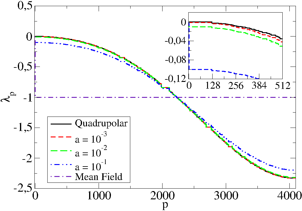
Figure 9: Spectrum of eigenvalues of elastic propagators: Mean-Field (MF), quadrupolar interaction and MF-weighted quadrupolar interactions. Eigenvalues are here simply ranked in the decreasing order. The introduction of a fraction $a$ of MF opens a gap between the translational mode having a null eigenvalue and the other modes $\lambda<0$. The evolution of the gap is zoomed in the inset.

In the quadrupolar case, a set of non-trivial eigenmodes are also characterized by a null eigenvalue. Namely ${\mathbf{e}}_{p,p}=e^{-i\frac{2\pi p(m+n)}{N}}$ and ${\mathbf{e}}_{p,-p}=e^{-i\frac{2\pi p(m-n)}{N}}$ with $p\in[-N/2,N/2-1]\backslash\{0\}$. Thus there is one trivial zero translation eigenmode and $2(N-1)$ non-trivial ones.

Let us rewrite the the plastic strain field in the Fourier basis using the more condensed form:

$$\varepsilon^{pl}=\sum_{p,q}c_{pq}{\mathbf{e}}_{p,q}\;,\quad\mathrm{where}\quad c_{pq}=\frac{1}{N^{2}}\widetilde{\varepsilon^{pl}_{pq}}$$ (12)

In order to follow the evolution of the different modes we now rewrite in Fourier space the argument of the $\mathop{\mathcal{P}}(\cdot)$ function in the equation of evolution (1):

$$\begin{array}[]{l}{\mathcal{F}}\left[\sigma^{ext}+G^{el}*\varepsilon^{pl}(\mathbf{r},t)-\sigma^{c}(\mathbf{r},\varepsilon^{pl})\right]=\vspace{5pt}\\ \sigma^{ext}\delta_{p}\delta_{q}+\widetilde{G^{Q}_{pq}}\widetilde{\varepsilon^{pl}_{pq}}-\widetilde{\left[\sigma^{c}(\mathbf{r},\varepsilon^{pl}(\mathbf{r}))\right]_{pq}}\;.\end{array}$$ (13)

Ignoring for the moment the effect of the function $\mathop{\mathcal{P}}(\cdot)$ in Eq. (1) we thus get by Fourier transform the evolution of the contribution of the different modes:

$$\frac{\partial c_{pq}}{\partial t}=\delta_{p}\delta_{q}\sigma^{ext}+\lambda_{pq}\partial c_{pq}-\widetilde{\left[\sigma^{c}(\mathbf{r},\varepsilon^{pl}(\mathbf{r}))\right]_{pq}}$$ (14)

This rewriting thus enables us a better understanding of the diffusive-like behavior observed at long times for the plastic strain. In real space, the spatial coupling is induced by the non-local elastic interaction kernel, $G^{el}$, while the noise term is local. In the space of eigenmodes, the opposite character is observed, namely the restoring force is local, but noise is not. Since all eigenvalues are null or negatives (otherwise the dynamics would be unstable) a competition emerges between the relaxation of the eigenmodes induced by the elastic contribution and a random forcing due to the quenched noise contribution. In particular, at long times, the contribution of the soft modes becomes dominant since they are not submitted to relaxation. The diffusive-like behavior thus directly emerges from a competition between the different soft modes controlled by the quenched disorder.

The strong effect of a small MF contribution to the quadrupolar propagator can now be re-read as the consequence of the opening of a gap in the spectrum of eigenvalues, in other words to the vanishing of the soft modes. In Fig. 9, the spectra of eigenvalues of the stress redistribution kernel show the gradual gap opening due to the introduction of a MF contribution to the elastic quadrupolar interaction. The associated restoring elastic force brings back the model to the standard depinning phenomenology.

Note that this interpretation only holds if we ignore the $\mathop{\mathcal{P}}(\cdot)$ function that intervenes in Eq. 1. When a long integration time in considered, the loading contributes to a positive average that allows for such an interpretation. However, at short time scales, the positive part function unfortunately cannot be simply expressed in Fourier space. A similar situation appears in classical depinning models. The point is that for the latter ones, a long time integration gives a finite restoring force to any wavelength of manifold fluctuations.

IV.2 From Soft modes to shear-bands

In the present context of amorphous plasticity an appealing alternative representation of the soft modes is given by the unit shear-bands orientated along $\pm\pi/4$. One defines ${\mathbf{d}}_{k}$ such that ${\mathbf{d}}_{k}(m,n)=\delta_{m-n-k}$ and ${\mathbf{d}^{\prime}}_{k}(m,n)=\delta_{m+n-k}$ where $k\in[-N/2+1,N/2-1]$ and $\delta_{n}$ is the Kronecker symbol. Plastic shear bands thus directly appear as soft modes of the quadrupolar elastic interaction, because of the null eigenvalue, they don’t induce any internal stress.

We use this decomposition to rewrite the plastic strain field as:

$$\varepsilon^{pl}=\sum_{|p|\neq|q|}c_{pq}{\mathbf{e}}_{p,q}+\sum_{k}c_{k}{\mathbf{d}}_{k}+\sum_{k}c^{\prime}_{k}{\mathbf{d}^{\prime}}_{k}\;,$$ (15)

where the first sum gathers all modes of non-zero eigenvalues whereas the two last sums correspond to combinations of shear bands oriented at $\pm\pi/4$. Note however that the two systems of shear bands are not independent since the scalar products ${\mathbf{d}}_{k}.{\mathbf{d}^{\prime}}_{l}$ may be non zero. Here the amplitudes $c_{k}$ and $c^{\prime}_{k}$ roughly correspond to the mean plastic strain along the shear-bands ${\mathbf{d}}_{k}$ and ${\mathbf{d}^{\prime}}_{k}$ respectively. In the same spirit as above, accounting for the non-orthogobality between the two slip systems, it is possible to write the equation of evolution of the amplitudes of the shear-bands:

$$\frac{\partial c_{k}}{\partial t}+\frac{1}{N}\!\sum_{\ell}f_{k\ell}\frac{\partial c^{\prime}_{k}}{\partial t} = \sigma^{ext}\!-\frac{1}{N}\!\sum_{\mathbf{r}\in{\mathbf{d}}_{k}}\sigma^{c}[(\mathbf{r},\varepsilon^{pl}(\mathbf{r})]$$ (16)

$$\frac{\partial c^{\prime}_{k}}{\partial t}+\frac{1}{N}\!\sum_{\ell}f_{k\ell}\frac{\partial c_{k}}{\partial t} = \sigma^{ext}\!-\frac{1}{N}\!\sum_{\mathbf{r}\in{\mathbf{d}^{\prime}}_{k}}\sigma^{c}[(\mathbf{r},\varepsilon^{pl}(\mathbf{r})]$$

where in the present case of bands at $\pm\pi/4$, $f_{k\ell}/2=(k-l)\pmod{2}$.

As already discussed above, in absence of elastic restoring force in the equation of evolution, we expect the strain field to be asymptotically dominated by the sole superimposition of soft modes, which we interpret here as shear bands at $\pm\pi/4$.

Here we obtain for the dynamics of the bands an advection contribution due to the differnce $(\sigma^{ext}-\overline{\sigma^{c}})$ between the driving force and the spatial average of the threshold on the whole lattice. In addition, the average along the bands of the fluctuating part of the thresholds and the inter-bands coupling introduce randomness and lead to diffusion.

Note that another important souce of interactions betwen bands has been neglected here. Although shear bands are expected to be dominant at long times, the short time synamics remains local. A natural consequence of the interplay between a local threshold dynamics and the non-local effects of the elastic interaction is the persistence of fluctuations along the bands. The convolution of the latter with the elastic kernel is responsible for a mechanical noise contribution in the dynamics Nicolas et al. (2014a); Jagla (2015); Agoritsas et al. (2015).

V Fluctuations and age statistics along shear-bands

The interpretation of the plastic shear-bands as soft modes of the elastic interaction encourages us to re-examine our results from this new perspective. In particular, we expect that at long times, plastic activity concentrates along weakly interacting shear bands. A natural question thus arises about the respective contribution of intra shear-bands and inter shear-bands fluctuations to the diffusive regime. This question is reminiscent of earlier studies showing anisotropic correlations in the plastic strain field Maloney and Robbins (2009); Talamali et al. (2012). In the same spirit, we suggested that the long sub-diffusive regime observed in the numerical results reflects an aging-like behavior. This motivates us to characterize age statistics inside and outside shear-bands.

We first define the mean variance of the plastic strain field inside the shear bands as:

$$W_{Q}^{+} = \langle\frac{1}{N}\sum_{k=1}^{N}W_{k}\rangle\;,\quad\mathrm{where}$$ (17)

$$W_{k} = \frac{1}{N}\sum_{{\mathbf{r}}\in{\mathbf{d}}_{k}}\left[\varepsilon^{pl}({\mathbf{r}})\right]^{2}-\left[\frac{1}{N}\sum_{{\mathbf{r}}\in{\mathbf{d}}_{k}}\varepsilon^{pl}({\mathbf{r}})\right]^{2}\;.$$

In the quadrupolar geometry associated to plane shear plasticity, the shear bands ${\mathbf{d}}_{k}$ and ${\mathbf{d}^{\prime}}_{k}$ are oriented along the $\pm\pi/4$ directions and receive a positive stress contribution whenever one of their site experiences plasticity, hence the superscript $+$ in the notation of the variance $W_{Q}^{+}$. In a similar spirit we can can characterize the fluctuations of the plastic strain field along the directions at angles $0$ and $\pi/2$ that receive a negative stress contribution when one of their site experiences plasticity. We denote $W_{Q}^{-}$ the variance of the plastic strain field along such negative stress directions.

We show in Fig. 10a the evolution of the global variance $W_{Q}$ of the plastic strain field as well as the variances $W_{Q}^{+}$ inside the shear-bands and $W_{Q}^{-}$ outside the shear-bands. We observe that the variance $W_{Q}^{+}$ of intra-shear-bands fluctuations are significantly lower than the global variance $W_{Q}$ in the diffusion regime. Conversely, the variance $W_{Q}^{-}$ measured in the negative stress directions is indistinguishable from the global variance. The inset shows the same data after rescaling by the mean plastic strain i.e. the effective diffusivities $D_{Q}=W_{Q}/\overline{\varepsilon_{pl}}$, $D_{Q}^{+}=W_{Q}^{+}/\overline{\varepsilon_{pl}}$ and $D_{Q}^{-}=W_{Q}^{-}/\overline{\varepsilon_{pl}}$. Here we see that the effective diffusivity within the shear-bands $D_{Q}^{+}$ is about two times smaller than the global diffusivity $D_{Q}$.

Beyond the spatial fluctuations, we can also characterize the temporal fluctuations. In order to do so, we define the local age variable ${\cal A}_{Q}=n_{A}/N^{2}$ that counts the number of plastic events $n_{A}$ that occurred in the system since the last time the site has experienced plasticity. In case of an homogeneous deformation, all $N^{2}$ sites would be expected to experience plastic events at the same frequency, hence the rescaling factor $1/N^{2}$. It is easy to extend this definition to a shear-band: ${\cal A}_{Q}^{+}=n_{A^{+}}/N$. Here $n_{A^{+}}$ is the number of plastic events since the last time a site of the band has experienced plasticity and the rescaling factor stems from the number $N$ of shear bands. The age ${\cal A}_{Q}^{-}$ of bands in the negative stress directions is defined in the very same way.

We show in Fig. 10b the distributions of ages $P(\log{\cal A_{Q}})$, $P(\log{\cal A}_{Q}^{+})$ and $P(\log{\cal A}_{Q}^{-})$ measured in the diffusive regime. The age distribution of sites $P(\log{\cal A_{Q}})$ peaks around unity and shows a cut-off around ten. This suggests that on average, the plastic activity is only moderately heterogeneous.

As for the spatial fluctuations we observe that the age statistics of bands $P({\cal A}_{Q}^{-})$ measured in negative stress directions (outside shear-bands) is close to the global age statistics $P({\cal A}_{Q})$ measured on individual sites. In contrast, the distribution $P({\cal A}_{Q}^{+})$ of ages of the shear-bands is shifted to larger values. A natural interpretation is that due to the positive stress redistribution, plastic activity remains trapped for longer periods within a shear-band (while the age of the other bands keeps increasing) before jumping to another one. We note in particular that the cut-off of the shear-band age distribution roughly corresponds to the duration of the subdiffusive regime.

The spatio-temporal fluctuations of the plastic activity within the shear-bands is thus clearly distinguishable from the backround. Still, this diference is not dramatic. Although the diffusivity is decreased and the duration of plastic activity is increased along the shear bands, the qualitative picture remains unchanged. Shear bands can survive 5-10 times longer than bands in the negative stress directions but the age statistics ends up converging toward a stationary distribution. This is for instance at contrast with the clear ergodicity breaking identified in Ref. Török et al. (2000).

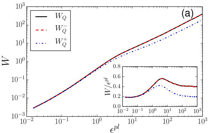
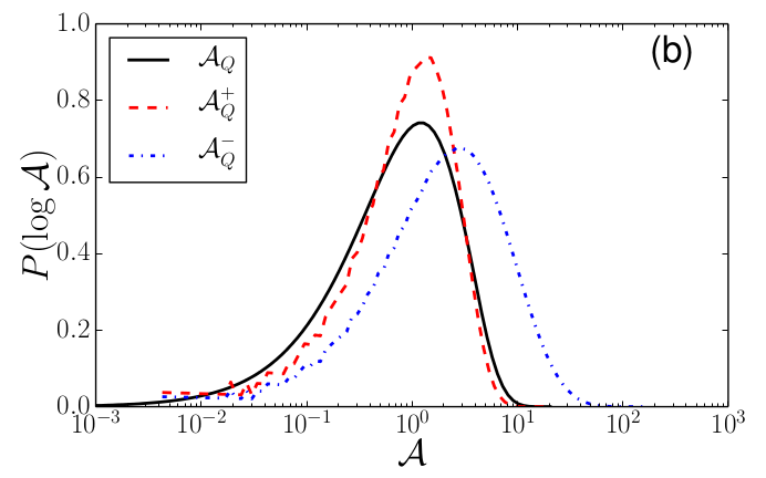
Figure 10: Quadripolar kernel. (a): variance of the plastic strain field inside and outside shear bands. (b): Age distribution inside and outside shear bands

VI Plane vs Antiplane shear in amorphous plasticity

A potential reason for the system to escape aging actually stems from the quadrupolar geometry of the elastic interaction at play in the present model. Since, after a plastic event, the elastic stress is positive along the two directions at $\pm\pi/4$, it is possible to trigger another plastic event in a direction at $0$ or $\pi$ with a sequence of two successive events at $+\pi/4$ then $-\pi/4$ (or the reverse). Such sequences thus restore some interaction between positive and negative stress directions.

In this section we follow this geometric idea by focussing on the case of antiplane shear geometry early studied in Ref. Baret et al. (2002). As mentioned above, in this antiplane geometry (defined in Fig 3b), a plastic inclusion induces a dipolar interaction:

$$G^{D}(r,\theta) \approx \frac{\cos 2\theta}{r^{2}}\;,\quad G^{D}(\mathbf{0})=-1$$ (18)

$$\widetilde{G^{D}_{pq}} = -2A\frac{q^{2}}{p^{2}+q^{2}}\;,\quad\widetilde{G^{D}_{00}}=0$$ (19)

Here the soft modes are shear-bands oriented at $\theta=0$ and the negative stress directions are oriented at $\theta=\pi$. In contrast with the previous quadrupolar case, no direct cross-talk mechanism is possible between the different shear-bands. This means in particular that if we now rewrite the plastic strain field as:

$$\varepsilon^{pl}=\sum_{|p|\neq 0}c_{pq}{\mathbf{e}}_{p,q}+\sum_{k}c^{D}_{k}{\mathbf{d}^{D}}_{k}\;,$$ (20)

where the $N$ horizontal bands ${\mathbf{d}^{D}}_{k}$ are the soft modes of the dipolar kernel $G^{D}$, we now obtain for the equation of evolution of the band amplitudes:

$$\frac{\partial c^{D}_{k}}{\partial t}=\sigma^{ext}-\frac{1}{N}\sum_{\mathbf{r}\in{\mathbf{d}^{D}}_{k}}\sigma^{c}[(\mathbf{r},\varepsilon^{pl}(\mathbf{r})]$$ (21)

We thus get in the long term dynamics a set of of bands that can grow independently of each other. Again, this statement has to be softened to account for the effective noise induced by the sort term local thershold dynamics that restore weak coupling between the bands.

In analogy with the previous section we show in Fig. 11a the evolution upon deformation of the variances $W_{D}^{+}$ and $W_{D}^{-}$ of the plastic strain field obtained along the positive and negative stress directions, respectively, in comparison with the global variance $W_{D}$. As in the quadrupolar case, the variance $W_{D}^{-}$ in the negative stress directions is almost the same as the global variance $W_{D}$. The result is strikingly different in the direction of shear-bands. After the power-law transient, instead of a diffusive regime, the variance $W_{D}^{+}$ shows indeed a clear saturation. Along the direction of the shear-bands, we thus recover the classical Family-Vicsek phenomenology of depinning. Note however that saturation is reached at a much later stage $\varepsilon^{pl}\approx 10$ than in the reference Mean-Field case $\varepsilon^{pl}\approx 0.5$ (see Fig. 4). If one refers to the results obtained with the composite kernels $G_{a}$ (see Fig. 7), this would correspond to small Mean-Field weight $a\approx 0.005$.

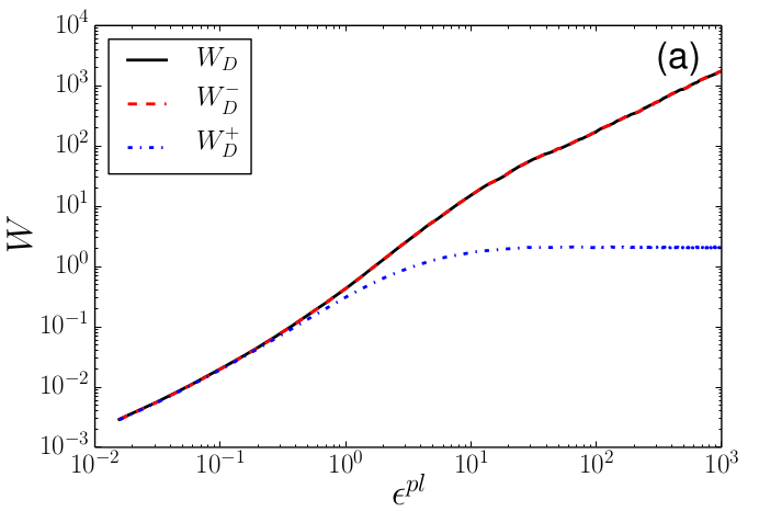
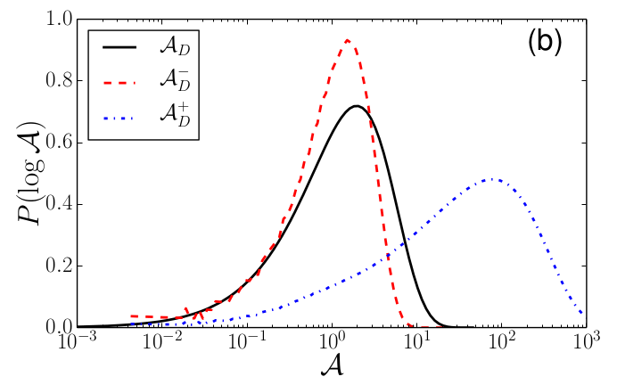
Figure 11: Aging and diffusive bhaviors obtained with a Dipolar kernel. (a): variance $W_{D}$ of the plastic strain field and variances $W_{D}^{+}$ inside and $W_{D}^{-}$ outside shear bands. (b): Age distributions $P(\log{\cal A}_{D})$ of the sites and and age distributions $P(\log{\cal A}_{D}^{+})$, $P(\log{\cal A}_{D}^{-})$ of the bands in the positive (shear-bands) and negative stress directions, respectively.

In Fig. 11b we show the distribution of ages in the antiplane shear geometry. Again, the age distribution $(\log{\cal A}_{D}^{-})$ of bands in the negative stress direction is very close to the age distribution $P(\log{\cal A}_{D})$ of the individual sites. The case of the shear-bands is strikingly different. Here the age distribution $P(\log{\cal A}_{D}^{+})$ is much older (about two orders of magnitude) than the two other ones. One recovers the same aging-like effect as for the shear-bands in the quadrupolar case but with a much higher amplitude.

VII Conclusion

Depinning models rely on the interplay between disorder and elasticity. While the yielding transition may be discussed within the framework of depinning, it appears that some specific properties of amorphous plasticity (diffusion, shear-banding) are controlled by the peculiar form of the quadrupolar elastic interaction. In order such features to be recovered in the framework of discrete lattice models, the discretized implementation of the Eshelby kernel has to preserve a key property of continuum plasticity: a unit plastic strain along any band in a direction of maximum shear stress (here $\pm\pi/4$) induces no residual stress.

The interpretation of the shear-bands as soft modes of the Eshelby elastic interaction may clarify the long debate about the relative importance of localized rearrangements and large scale shear-band like events Tanguy et al. (2006),Dasgupta et al. (2012); *Ashwin-PRE13; *Dasgupta-PRE13a as microscopic mechanisms of amorphous plasticity and complex rheology. It appears in particular that localized plastic events is the rule at short time scales but on a larger time horizon, mostly shear bands account for the kinematics, as these are the only displacement fields that prevent large shear stress build-up.

While the present study has been concerned with the modeling of amorphous media plasticity, a similar phenomenology is expected for any depinning model as soon as the elastic propagator exhibits soft modes. As discussed in Lin et al. (2014b) in the case of plastic yielding, this new sub-class of depinning model is expected to exhibit non-trivial scaling properties. More generally it is tempting to study in more details the ergodic behavior of such models at finite temperature in relation with the Soft Glassy Rheology models Sollich et al. (1997); *Sollich-PRE98 and with the recent observation of the strong effect of Eshelby events on relaxation processes in the liquid state Lemaître (2014).