Covariance Matrices and Influence Scores for Mean Field Variational Bayes

Abstract

Mean field variational Bayes (MFVB) is a popular posterior approximation method due to its fast runtime on large-scale data sets. However, it is well known that a major failing of MFVB is that it underestimates the uncertainty of model variables (sometimes severely) and provides no information about model variable covariance. We develop a fast, general methodology for exponential families that augments MFVB to deliver accurate uncertainty estimates for model variables—both for individual variables and coherently across variables. MFVB for exponential families defines a fixed-point equation in the means of the approximating posterior, and our approach yields a covariance estimate by perturbing this fixed point. Inspired by linear response theory, we call our method linear response variational Bayes (LRVB). We also show how LRVB can be used to quickly calculate a measure of the influence of individual data points on parameter point estimates. We demonstrate the accuracy and scalability of our method by learning Gaussian mixture models for both simulated and real data.

1 Introduction

With increasingly efficient data collection methods, scientists are interested in quickly analyzing ever larger data sets. In particular, the promise of these large data sets is not simply to fit old models but instead to learn more nuanced patterns from data than has been possible in the past. In theory, the Bayesian paradigm promises exactly these desiderata. Hierarchical modeling allows practitioners to capture complex relationships between variables of interest. Moreover, Bayesian analysis allows practitioners to quantify the uncertainty in any model estimates—and to do so coherently across all of the model variables.

Mean field variational Bayes (MFVB), a method for approximating a Bayesian posterior distribution, has grown in popularity due to its fast runtime on large-scale data sets [1, 2, 3]. But it is well known that a major failing of MFVB is that it gives underestimates of the uncertainty of model variables that can be arbitrarily bad, even when approximating a simple multivariate Gaussian distribution [4, 5, 6], and provides no information about how the uncertainties in different model variables interact [7, 5, 8, 6]. We develop a fast, general methodology for exponential families that augments MFVB to deliver accurate uncertainty estimates for model variables—both for individual variables and coherently across variables. In particular, as we elaborate in Section 2, MFVB for exponential families defines a fixed-point equation in the means of the approximating posterior, and our approach yields a covariance estimate by perturbing this fixed point. The perturbations of linear response theory have previously been applied for machine learning by [9] and specifically for mean-field methods by [10] and [11]. Our contribution is to use exponential families to derive particularly simple and scalable formulas for covariance estimation and to develop a method to quickly calculate influence scores, which measure the influence of individual data points on parameter point estimates. We call our method linear response variational Bayes (LRVB).

We demonstrate the accuracy and scalability of our LRVB covariance estimates with experiments that focus on finite mixtures of multivariate Gaussians, which have historically been a sticking point for MFVB covariance estimates [5, 6]. We employ simulated data as well as the MNIST handwritten digit data set [12]. We show that the LRVB variance estimates are nearly identical to those produced by a Markov Chain Monte Carlo (MCMC) sampler, even when MFVB variance is dramatically underestimated. For these mixture models, we show that LRVB gives accurate covariance estimates orders of magnitude faster than MCMC on a wide range of problems. We demonstrate both theoretically and empirically that, for this Gaussian mixture model, LRVB scales linearly in the number of data points and approximately quadratically in the dimension of the parameter space. Finally, we show how LRVB allows fast computation of the influence scores mentioned above.

2 Mean-field variational Bayes in exponential families

Denote our $N$ observed data points by the $N$-long column vector $x$, and denote our unobserved model parameters by $\theta$. Here, $\theta$ is a column vector residing in some space $\Theta$; it has $J$ subgroups and total dimension $D$. Our model is specified by a distribution of the observed data given the model parameters—the likelihood $p(x|\theta)$—and a prior distributional belief on the model parameters $p(\theta)$. Bayes’ Theorem yields the posterior $p(\theta|x)$.

MFVB approximates $p(\theta|x)$ by a factorized distribution of the form $q(\theta)=\prod_{j=1}^{J}q(\theta_{j})$ such that the Kullback-Liebler divergence $\textrm{KL}(q||p)$ between $q$ and $p$ is minimized:

$$q^{*} :=\operatorname*{arg\,min}_{q}\textrm{KL}(q||p)$$

$$=\operatorname*{arg\,min}_{q}\mathbb{E}_{q}\left[\log p(\theta|x)-\sum_{j=1:J}\log q(\theta_{j})\right].$$

By the assumed $q$ factorization, the solution to this minimization obeys the following fixed point equations [5]:

$$\log q^{*}_{j}(\theta_{j})=\mathbb{E}_{q^{*}_{i}:i\in[J]\setminus j}\log p(\theta,x)+C.$$ (1)

Here, and for the rest of the text, $C$ denotes a constant and $[J]:=\{1,\ldots,J\}$. For index $j$, suppose that $p(\theta_{j}|\theta_{i\in[J]\setminus j},x)$ is in natural exponential family form:

$$p(\theta_{j}|\theta_{i\in[J]\setminus j},x)=\exp(\tilde{\eta}_{j}^{T}\theta_{j}-A_{j}(\tilde{\eta}_{j}))$$ (2)

with local natural parameter $\tilde{\eta}_{j}$ and local log partition function $A_{j}$. Here, $\tilde{\eta}_{j}$ may be a function of $\theta_{i\in[J]\setminus j}$ and $x$. If the exponential family assumption above holds for every index $j$, then we can write $\tilde{\eta}_{j}$ as a sum of products of components of each $\theta_{k}$ vector:

$$\tilde{\eta}_{j}=\sum_{r\in R_{j}}G_{r}\prod_{k\in[J]\setminus j}\theta_{kr_{k}},$$ (3)

where $G_{r}$ is a $D_{j}$-sized column vector and $\theta_{kr_{k}}$ is a scalar. Here, $r$ is a vector of length $J-1$. Each entry $r_{k}$ of $r$ is either $\emptyset$ or an index in $[D_{k}]$. If $r_{k}=\emptyset$, then $\theta_{kr_{k}}=1$; otherwise, $\theta_{kr_{k}}$ is the $r_{k}$th element of the vector $\theta_{k}$. This notation scheme guarantees that each product contains at most one factor from the vector $\theta_{k}$ for each index $k$. In particular, the log likelihood is linear in every vector $\theta_{j}$. This property of the log likelihood is guaranteed by Eq. (2). Appendix A.1 contains further details and a proof of Eq. (3).

It follows from Eqs. (1), (2), (3), and the assumed factorization of $q^{*}$ that $\log q^{*}_{j}(\theta_{j})$ has the form

$$\left(\sum_{r\in R_{j}}G_{r}\prod_{k\in[J]\setminus j}\mathbb{E}_{q^{*}_{r}}[\theta_{kr_{k}}]\right)^{T}\theta_{j}+C.$$ (4)

We see that $q^{*}_{j}$ is in the same exponential family form as $p(\theta_{j}|\theta_{i\in[J]\setminus j},x)$. Let $\eta_{j}$ denote the natural parameter of $q^{*}_{j}$, and denote the mean parameter of $q^{*}_{j}$ as $m_{j}:=\mathbb{E}_{q^{*}_{j}}\theta_{j}$. We see from Eq. (4) that

$$\eta_{j}=\sum_{r\in R_{j}}G_{r}\prod_{k\in[J]\setminus j}m_{kr_{k}}.$$

Since $m_{j}$ is a function of $\eta_{j}$, we have the fixed point equations $m_{j}:=M_{j}(m_{i\in[J]\setminus j})$ for mappings $M_{j}$ across $j$ and

$$m:=M(m)$$

for the vector of mappings $M$.

3 Linear response covariance estimation

Let $V$ denote the covariance matrix of $\theta$ under the factorized variational distribution $q^{*}(\theta)$, and let $\Sigma$ denote the covariance matrix of $\theta$ under the true distribution, $p(\theta|x)$:

$$V:=\textrm{Cov}_{q^{*}}\theta,\quad\quad\Sigma:=\textrm{Cov}_{p}\theta.$$

$V$ may be a poor estimate of $\Sigma$, even when $m\approx\mathbb{E}_{p}\theta$, i.e. when the marginal means match well [4, 7, 5, 8, 6]. Our goal is to use the MFVB solution and the techniques of linear response theory [9, 10, 11] to construct an improved estimate for $\Sigma$.

Define $p_{t}(\theta|x)$ such that its log is a linear perturbation of the log posterior:

$$\log p_{t}(\theta|x)=\log p(\theta|x)+t^{T}\theta-C(t),$$ (5)

where $C(t)$ is a constant in $\theta$. If we assume that $p(\theta|x)$ is a probability distribution with natural parameters in the interior of the feasible space, then $p_{t}(\theta|x)$ is a probability distribution for any $t$ in an open ball around $0$. Since $C(t)$ normalizes the $p_{t}(\theta|x)$ distribution, it is in fact the cumulant generating function of $p(\theta|x)$. Further, every (perturbed) conditional distribution $p_{t}\left(\theta_{j}|\theta_{i\in[J]\setminus j},x\right)$ is in the same exponential family as every (unperturbed) conditional distribution $p\left(\theta_{j}|\theta_{i\in[J]\setminus j},x\right)$ by construction. So, for each $t$, we have mean field variational approximation $q_{t}^{*}$ with marginal means $m_{t,j}:=E_{q_{t}^{*}}\theta_{j}$ and fixed point equations $m_{t,j}=M_{t,j}(m_{t,i\in[J]\setminus j})$ across $j$. Thus, $m_{t}=M_{t}(m_{t})$ as in Section 2. Taking derivatives of the latter relationship with respect to $t$, we find

$$\frac{dm_{t}}{dt^{T}}=\frac{\partial M_{t}}{\partial m_{t}^{T}}\frac{dm_{t}}{dt^{T}}+\frac{\partial M_{t}}{\partial t^{T}}.$$ (6)

In particular, note that $t$ is a vector of size $D$ (the total dimension of $\theta$), and $\frac{dm_{t}}{dt^{T}}$, e.g., is a matrix of size $D\times D$ with $(a,b)$th entry equal to the scalar $dm_{t,a}/dt_{b}$.

Since $q_{t}^{*}$ is the MFVB approximation for the perturbed posterior $p_{t}(\theta|x)$, we may hope that $m_{t}=E_{q_{t}^{*}}\theta$ is close to the perturbed-posterior mean $\mathbb{E}_{p_{t}}\theta$. The practical success of MFVB relies on the fact that this approximation is often good in practice. To derive interpretations of the individual terms in Eq. (6), we assume that this equality of means holds, but we indicate where we use this assumption with an approximation sign: $m_{t}\approx\mathbb{E}_{p_{t}}\theta$. The full derivations of the following equations are given in Appendix A.2.

$$\frac{dm_{t}}{dt^{T}} \approx\frac{d}{dt^{T}}\mathbb{E}_{p_{t}}\theta=\Sigma_{t}$$ (7)

$$\frac{\partial M_{t}}{\partial t^{T}} =\frac{\partial}{\partial t^{T}}\mathbb{E}_{q_{t}^{*}}\theta=V_{t}$$ (8)

$$\frac{dM_{t}}{dm_{t}^{T}} =V_{t}H_{t},$$ (9)

where $\Sigma_{t}$ is the covariance matrix of $\theta$ under $p_{t}$, $V_{t}$ is the covariance matrix of $\theta$ under $q_{t}^{*}$, and

$$H_{t}:=E_{q^{*}}\left(\frac{\partial^{2}\log p_{t}(\theta|x)}{\partial\theta\partial\theta^{T}}\right)$$

Then substituting Eqs. (7), (8), and (9) into Eq. (6), evaluating at $t=0$, and writing $H$ for $H_{0}$ and $V$ for $V_{0}$, we find

$$\hat{\Sigma} := \left.\frac{dm_{t}}{dt^{T}}\right|_{t=0}\approx\Sigma$$

$$\hat{\Sigma} = VH\hat{\Sigma}+V\Rightarrow$$

$$\hat{\Sigma} = (I-VH)^{-1}V$$ (10)

Thus, we call $\hat{\Sigma}$ the LRVB estimate of the true posterior covariance $\Sigma$.

3.1 Exactness of multivariate normal and SEM

Consider approximating a multivariate normal posterior distribution $p(\theta|x)$ with MFVB. This case arises, for instance, given a multivariate normal likelihood with fixed covariance $S$ and an improper uniform prior on the mean parameter $\mu$:

$$p(x|\mu)=\prod_{n=1:N}\mathcal{N}(x_{n}|\mu,S)\;\textrm{ and }\;q^{*}(\mu)=\prod_{j=1:J}q^{*}_{j}(\mu_{j})$$

Here, $\mathcal{N}$ represents the multivariate normal distribution, and the total dimension $D$ of $\mu$ is equal to the number of components $J$. So $\mu$ is a $J$-length vector for $J>1$ with elements $\mu_{1},...,\mu_{J}$, and $S$ is a known $J\times J$ positive definite matrix. Our variational approximation, $q^{*}$, is given by the factorized distribution over mean components.

In this case, it is well known that the MFVB posterior means are correct, but the marginal variances are underestimated if $S$ is not diagonal. This fact is often used to illustrate the shortcomings of MFVB [4, 7, 5, 6].

However, since the posterior means are correctly estimated, the LRVB approximation in Eq. (10) is in fact an equality. That is, for the posterior location of a multivariate normal with known covariance, Eq. (10) is not an approximation, and $\hat{\Sigma}=\frac{dm_{t}}{dt^{T}}=\Sigma$ exactly. A detailed proof of this fact can be found in Appendix B.

This result draws a connection between LRVB and the “supplemented expectation-maximization” (SEM) method of [13]. SEM is an asymptotically exact covariance correction for the EM algorithm that transforms the full-data Fisher information matrix into the observed-data Fisher information matrix using a correction that is formally similar to Eq. (10). In this sense, SEM is a frequentist perspective on a special case of the LRVB correction when the amount of data goes to infinity. More details can be found in Appendix B.

4 Scaling

Eq. (10) requires the inverse of a matrix as large as all the unknown natural parameters in the posterior $p(\theta|x)$, which generally includes both main parameters and nuisance parameters. In many applications, the number of nuisance parameters may be very large. For example, in the finite mixture of normals model below (Section 6), there is an indicator variable for the cluster assignment for each data point. If we treat these variables as nuisance parameters, the number of nuisance parameters grows with the number of data points $N$. As a result, directly computing the matrix inverse in Eq. (10) may be impractical.

However, since the variational covariance $V$ is block diagonal and $H$ is often sparse, one may be able to use Schur complements to efficiently calculate sub-matrices of $\hat{\Sigma}$. Suppose that our full parameter space, $\theta$, can be divided into a small number of variables of primary interest, called $\alpha$, and a large (and possibly growing) number of nuisance variables, $z$:

$$\theta=\left(\begin{array}[]{c}\alpha\\ z\end{array}\right),\quad\quad\Sigma=\left[\begin{array}[]{cc}\Sigma_{\alpha}&\Sigma_{\alpha z}\\ \Sigma_{z\alpha}&\Sigma_{z}\end{array}\right].$$

We can similarly define partitions for $H$ and $V$. Assume also that we have the usual mean field factorization of the variational approximation: $q^{*}(\alpha,z)=q^{*}(\alpha)q^{*}(z)$, so that $V_{\alpha z}=0$. (The variational distributions may factor further as well.) We calculate the Schur complement of $\hat{\Sigma}$ in Eq. (10) with respect to its $z$th component to find that

$$\hat{\Sigma}_{\alpha}=$$ (11)

$$\quad(I_{\alpha}-V_{\alpha}H_{\alpha}-V_{\alpha}H_{\alpha z}\left(I_{z}-V_{z}H_{z})^{-1}V_{z}H_{z\alpha}\right)^{-1}V_{\alpha}$$

Here, $I_{\alpha}$ and $I_{z}$ refer to $\alpha$- and $z$-sized identity matrices, respectively. A detailed derivation can be found in Appendix A.2. In cases where $\left(I_{z}-V_{z}H_{z}\right)^{-1}$ can be efficiently calculated, Eq. (11) involves only an $\alpha$-sized inverse. A finite mixture of Gaussians model, which we describe in Section 6, is one such case.

5 Influence scores

Influence scores are a powerful tool from classical linear regression that describe how much influence a particular data point has on a modeled outcome. They can be used, for example, to identify outliers and investigate the robustness of the linear model [14, 15]. Analogously, it can be useful know how much Bayesian posterior means depend on the values of individual data points. A number of authors have proposed methods to measure the sensitivity of the posterior distribution to perturbations or deletions of data points both in linear models [16, 17] and more generally [18, 19, 20]. LRVB gives a convenient formula to analytically calculate the influence of individual data points as covariances between the $\theta$ vector and infinitesimal noise added to the data.

Consider the conditional expectation of a single parameter value, $\theta_{i}$, as a function of a single data point, $x_{n}$. Specifically, for notational convenience, define

$$m_{\theta_{i}}\left(x_{n}\right) = \mathbb{E}_{p}\left[\theta_{i}|x_{1},...,x_{n},...,x_{N}\right]$$

One measure of the sensitivity of $\theta_{i}$ to $x_{n}$ is the derivative of this function, $\frac{d}{dx_{n}}m_{\theta_{i}}\left(x_{n}\right)=m_{\theta_{i}}^{\prime}\left(x_{n}\right)$. We will refer to this derivative as an influence score for Bayesian models.

To draw a connection between this influence score and covariances, imagine that our observations, $x$, are in fact slightly noisy versions of the true data, $x^{*}$. Specifically, our model becomes

$$p(x|x^{*},\theta)=p(x|x^{*})p(x^{*}|\theta).$$

In this new model, $x^{*}$ are unknown parameters, like $\theta$. We assume our posterior beliefs about the true $x^{*}$ obey the following assumptions:

$$\mathbb{E}\left(x^{*}|x\right) = x$$

$$\textrm{Cov}\left(x^{*}|x\right) = \Sigma_{x}$$ (12)

$$S_{x} := \lim_{\epsilon\rightarrow 0}\frac{1}{\epsilon}\Sigma_{x}$$

$$0\neq S_{x} < \infty$$

Higher moments $$= O\left(\epsilon^{p}\right)\textrm{, for }p>2$$

That is, the covariance matrix $\Sigma_{x}$ is proportional to $\epsilon$. Conditional on $x$, $m_{\theta_{i}}\left(x_{i}^{*}\right)$ is a random variable that varies as the posterior belief about $x_{i}^{*}$ varies around $x_{i}$. By forming a Taylor expansion of $m_{\theta_{i}}^{\prime}(x^{*}_{n})$ around $x_{n}$ we show for any data point $x_{n}$ and any parameter $\theta_{i}$ that:

$$m_{\theta_{i}}^{\prime}\left(x_{n}\right) =\lim_{\epsilon\rightarrow 0}\frac{1}{\epsilon}\textrm{Cov}\left(\theta_{i},x_{n}^{*}|x\right)$$ (13)

(Appendix D contains further details.) That is, the limiting value of this covariance as $\epsilon\rightarrow 0$ can be used to estimate the influence of observation $x_{n}$ on the mixture parameters in the spirit of classical linear model influence scores from the statistics literature.

Note that the covariances on the right hand side of Eq. (13) are impossible to compute in naive MFVB, since they involve correlations between distinct mean field components, and difficult to compute using MCMC, since they require estimating a large number of very small covariances with a finite number of draws. However, LRVB leads to a straightforward analytic expression for these covariances.

To derive the LRVB influence scores, we now assume that the parameter space of the posterior can be divided into three types of variables. We have main and nuisance parameters, called $\alpha$ and $z$ respectively as in Section 4, and now also $x^{*}$, the unobserved data. As before, we also assume that each has its own variational distribution, i.e. $q^{*}(\theta)=q^{*}(\alpha)q^{*}(z)q^{*}(x^{*})$. (The variational distributions may factor still further.) We can write:

$$\theta=\left(\begin{array}[]{c}\alpha\\ x^{*}\\ z\end{array}\right)\quad\textrm{ and }\quad\Sigma=\left[\begin{array}[]{ccc}\Sigma_{\alpha}&\Sigma_{\alpha x^{*}}&\Sigma_{\alpha z}\\ \Sigma_{x^{*}\alpha}&\Sigma_{x^{*}}&\Sigma_{x^{*}z}\\ \Sigma_{z\alpha}&\Sigma_{zx^{*}}&\Sigma_{z}\end{array}\right].$$

We use a similar partition for $V$ and $H$. Recall that $\Sigma_{x}$ is the result of an infinitesimal perturbation and nearly zero, so we express our results in terms of $S_{x}$ in Eq. (5). Let $\Sigma_{\alpha}$ denote the the ordinary LRVB covariance of $\alpha$ from Eq. (11). The covariance between $\alpha$ and the infinitesimally perturbed $x$ then has the following formula:

$$\lim_{\epsilon\rightarrow 0}\frac{1}{\epsilon}\Sigma_{\alpha x^{*}}=$$ (14)

$$\quad\Sigma_{\alpha}^{-1}(V_{\alpha}H_{\alpha x^{*}}+V_{\alpha}H_{\alpha z}\left(I_{z}-V_{z}H_{z}\right)^{-1}V_{z}H_{zx^{*}})S_{x}$$

This formula follows from the Schur inverse and taking $\epsilon\rightarrow 0$. Details can be found in Appendix D.

6 Experiments

Mixture models constitute some of the most popular models for MFVB application [1, 2] and are often used as an example of where MFVB covariance estimates may go awry [5, 6]. We thus illustrate the efficacy of LRVB on the problem of approximating the posterior when the likelihood is a finite mixture of multivariate Gaussians.

6.1 Model

We consider a $K$-component mixture of $P$-dimensional multivariate normals with unknown component means, covariances, and weights. In what follows, the weight $\pi_{k}$ is the probability of the $k$th component, $\mathcal{N}$ denotes the multivariate normal distribution, $\mu_{k}$ is the $P$-dimensional mean of the $k$th component, and $\Lambda_{k}$ is the $P\times P$ precision matrix of the $k$th component (so $\Sigma_{k}:=\Lambda_{k}^{-1}$ is the covariance). $N$ is the number of data points, and $x_{n}$ is the $n$th observed $P$-dimensional data point. We employ the standard trick of augmenting the data generating process with the latent indicator variables $z_{nk}$, where $n=1,...,N$ and $k=1,...,K$, and

$$P(z_{nk}=1) = \pi_{k}$$

$$z_{nk}=1 \Rightarrow x_{n}\sim\mathcal{N}(\mu_{k},\Lambda^{-1}_{k})$$

The full likelihood under this augmentation is

$$p(x|\pi,\mu,\Lambda,z)=\prod_{n=1:N}\prod_{k=1:K}\mathcal{N}(x_{n}|\mu_{k},\Lambda^{-1}_{k})^{z_{nk}}$$ (15)

We assign independent variational factors to $\mu$, $\pi$, $\Lambda$, and $z$. The $z$ variables are nuisance parameters.

Our goal is to estimate the covariance matrix of the parameters $\log(\pi),\mu,\Lambda$ in the posterior distribution $p(\pi,\mu,\Lambda|x)$ and to estimate the influence of each data point $x_{n}$ on the posterior means of $\log(\pi),\mu,\Lambda$ using LRVB (see Sections 3 and 5).

In addition to the standard MFVB covariance matrices, we will compare the accuracy and speed of our estimates to Gibbs sampling on the augmented model (Eq. (15)) using the function rnmixGibbs from the R package bayesm. Our LRVB implementation relied heavily on linear algebra routines in RcppEigen [21]. We evaluate our results both on simulated data and on the MNIST data set [12].

6.2 MNIST data set

For a real-world example, we applied LRVB to the unsupervised classification of two digits from the MNIST dataset of handwritten digits. We first preprocess the MNIST dataset by performing principle component analysis on the training data’s centered pixel intensities and keeping the top $25$ components. For evaluation, the test data is projected onto the same $25$-dimensional subspace found using the training data.

We then treat the problem of separating handwritten $0$s from $1$s as an unsupervised clustering problem. We limit the dataset to instances labeled as $0$ or $1$, resulting in $12665$ training and $2115$ test points. We fit the training data as a mixture of multivariate Gaussians. Here, $K=2$, $P=25$, and $N=12665$. Then, keeping the $\mu$, $\Lambda$, and $\pi$ parameters fixed, we calculate the expectations of the latent variables $z$ in Eq. (15) for the test set. We assign test set data point $x_{n}$ to whichever component has maximum a posteriori expectation. We count successful classifications as test set points that match their cluster’s majority label and errors as test set points that are different from their cluster’s majority label. By this measure, our test set error rate was $0.08$. We stress that we intend only to demonstrate the feasibility of LRVB on a large, real-world dataset rather than to propose practical methods for modeling MNIST.

6.3 Covariance experiments

In this section, we check the covariances estimated with Eq. (10) against a Gibbs sampler, which we treat as the ground truth.

For simulations, we generated $N=10000$ data points from $K=2$ multivariate normal components in $P=2$ dimensions. MFVB is expected to underestimate the marginal variance of $\mu$, $\Lambda$, and $\log(\pi)$ when the components overlap since that induces correlation in the posteriors due to the uncertain classification of points between the clusters. These correlations are in violation of the MFVB assumption and cause the MFVB posterior variances to be mis-estimated.

We performed $68$ simulations, each of which had at least $500$ effective Gibbs samples in each variable—calculated with the R tool effectiveSize from the coda package [22]. We note that for each of the parameters $\log(\pi)$, $\mu$, and $\Lambda$, both MH and MFVB produce posterior means close to the ground truth MCMC values, so our key assumption in the LRVB derivations of Section 3 appears to hold.

Each point in Fig. (1) represents the a single parameter in a single simulation. For example, each point on the $\Lambda$ graph represents the marginal standard deviation of a particular component of the $\Lambda$ matrix for both the Gibbs sample and an alternative method. The first three graphs show the diagonal standard deviations, and the final graph shows the off-diagonal covariances. Note that the final graph excludes the MFVB estimates since most of the values are zero.

Fig. (1) shows that the raw MFVB covariance estimates are often quite different from the Gibbs sampler results, while the LRVB estimates match the Gibbs sampler closely. Although not shown, the results on the MNIST dataset were as good.

In these simulations, on average LRVB took only $3.40$ seconds, whereas the Gibbs sampler took $306.97$ seconds. We explore these timing tradeoffs in more detail in Section 6.4.

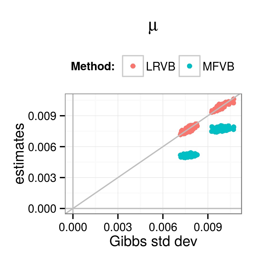
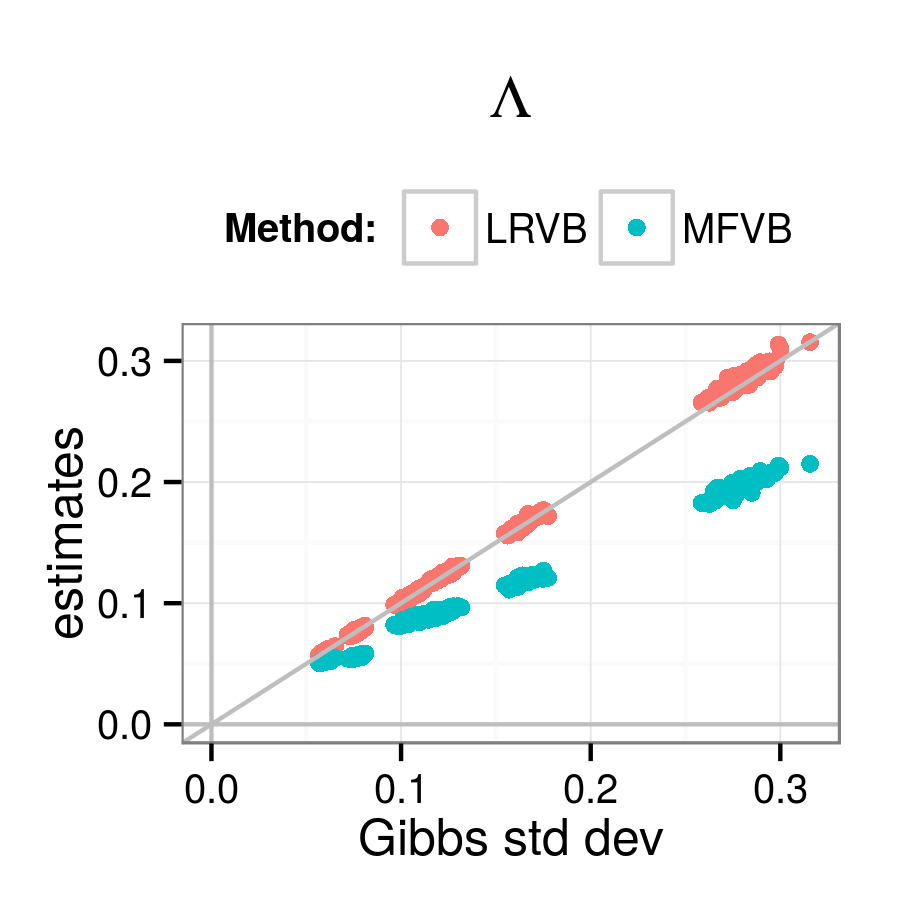
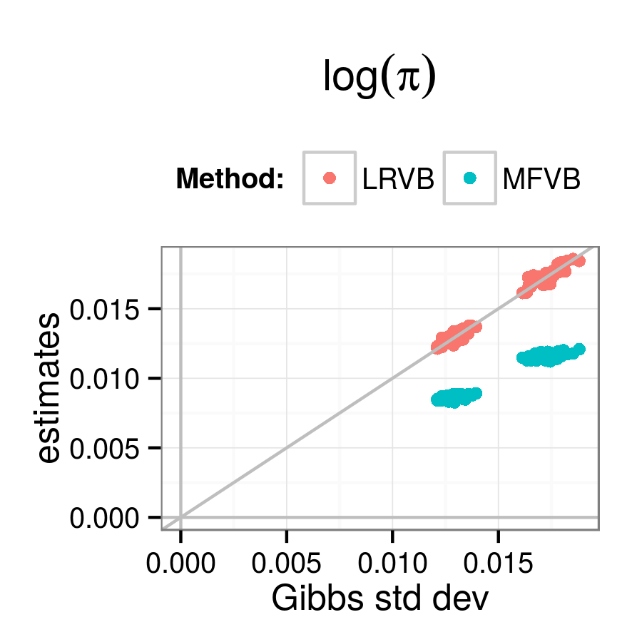
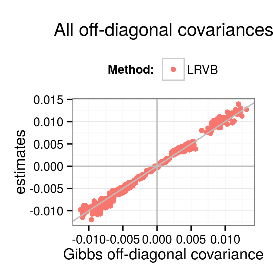
Figure 1: Comparison of estimates of the posterior covariance matrix on simulation data for each model parameter from Gibbs, MFVB, and LRVB methods. In the simulations, $N=10000$ (data points), $K=2$ (components) and $P=2$ (dimensions).

6.4 Scaling experiments

In this section we show that, for the finite mixture of multivariate Gaussians model, Eq. (10) scales linearly with $N$ and polynomially in $K$ and $P$. We also use simulations to experimentally compare the scaling of LRVB running times to Gibbs sampling estimates. We show that LRVB is much faster than Gibbs for the range of parameters we simulated, though Gibbs may be preferable for very high-dimensional problems.

In the terms of Section 4, $\alpha$ includes the sufficient statistics from $\mu$, $\pi$, and $\Lambda$, and grows as $O(KP^{2})$. The sufficient statistics for the variational posterior of $\mu$ contain the $P$-length vectors $\mu_{k}$, for each $k$, and the $(P+1)P/2$ second-order products in the covariance matrix $\mu_{k}\mu_{k}^{T}$. Similarly, for each $k$, the variational posterior of $\Lambda$ involves the $(P+1)P/2$ sufficient statistics in the symmetric matrix $\Lambda_{k}$ as well as the term $\log|\Lambda_{k}|$. The sufficient statistics for the posterior of $\pi_{k}$ are the $K$ terms $\log\pi_{k}$. This means that, minimally, Eq. (10) will require the inverse of a matrix of size $O(KP^{2})$.

The sufficient statistics for $z$ have dimension $K\times N$. In other words, the number of nuisance parameters grows with the number of data points, but $H_{z}=0$ for the multivariate normal (Appendix C contains further details), so we can apply Eq. (11) to replace the inverse of an $O(KN)$-sized matrix with multiplication by an $O(KN)$-sized matrix. Here, $z$ conveniently corresponds directly to the $z$ in Section 4.

Since a matrix inverse is cubic in the size of the matrix, the worst-case scaling for LRVB is then $O(K^{2})$ in $K$, $O(P^{6})$ in $P$ and $O(N)$ in $N$.

In our simulations, shown in Fig. (2), we can see that, in practice, LRVB scales linearly in $N$ and slightly less than quadratically in $P$, which is much better than the theoretical worst case. Note that the vertical axis, the time to run the algorithm, is on the log scale. At every value of $P$, $K$, and $N$ examined here, calculating LRVB is much faster than Gibbs sampling.

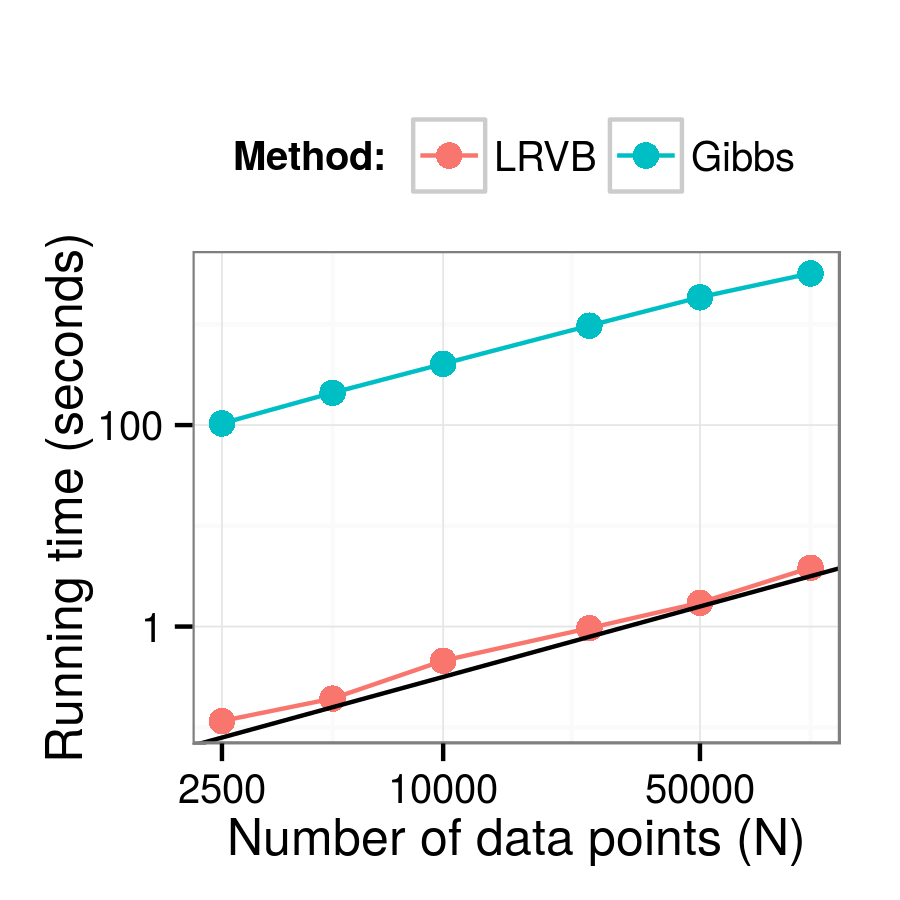
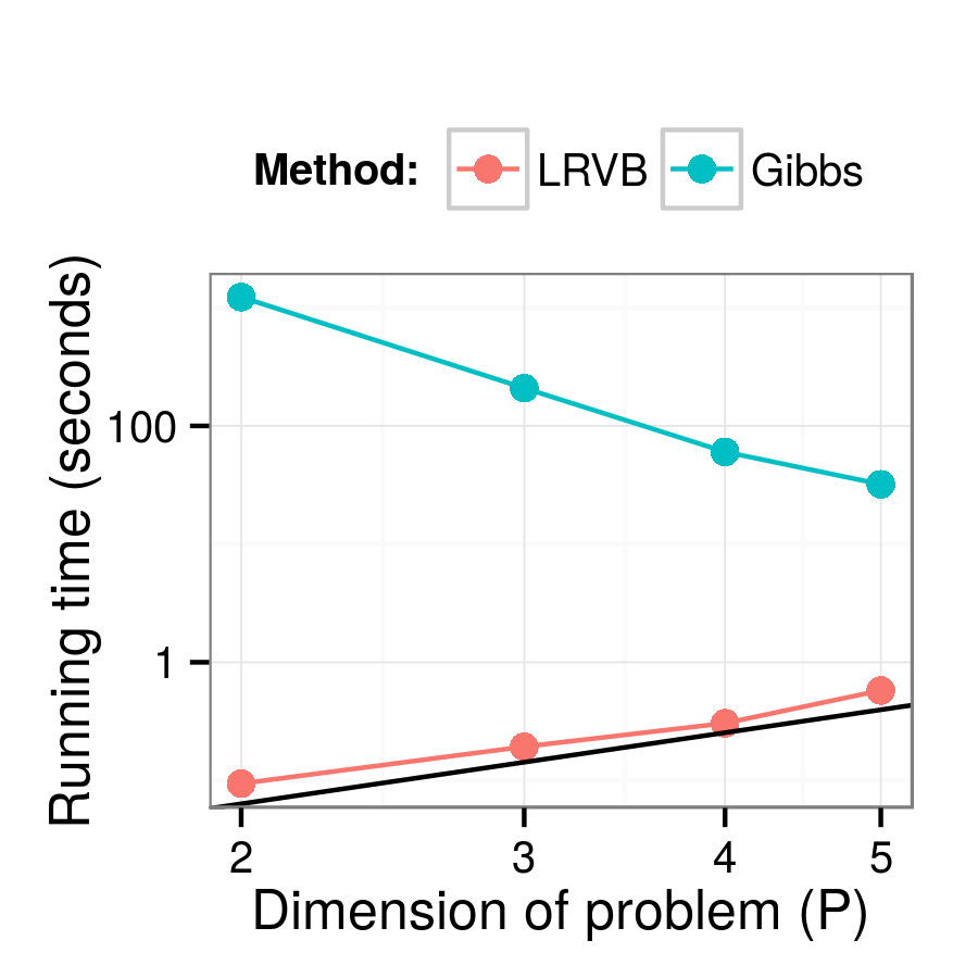
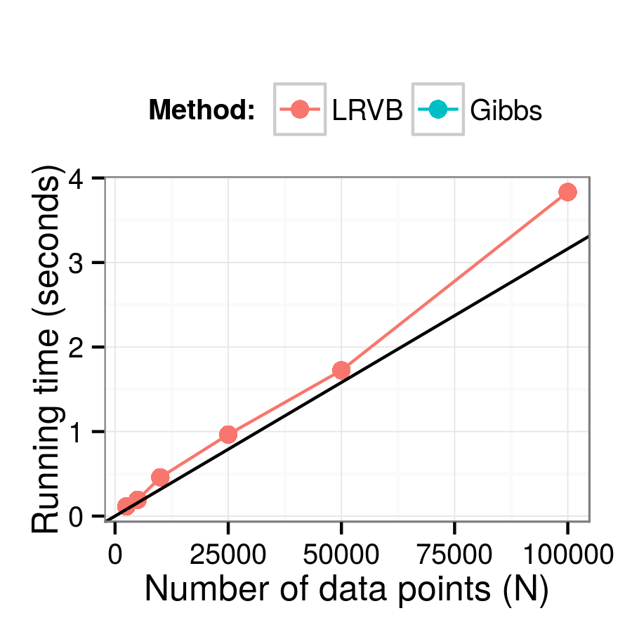
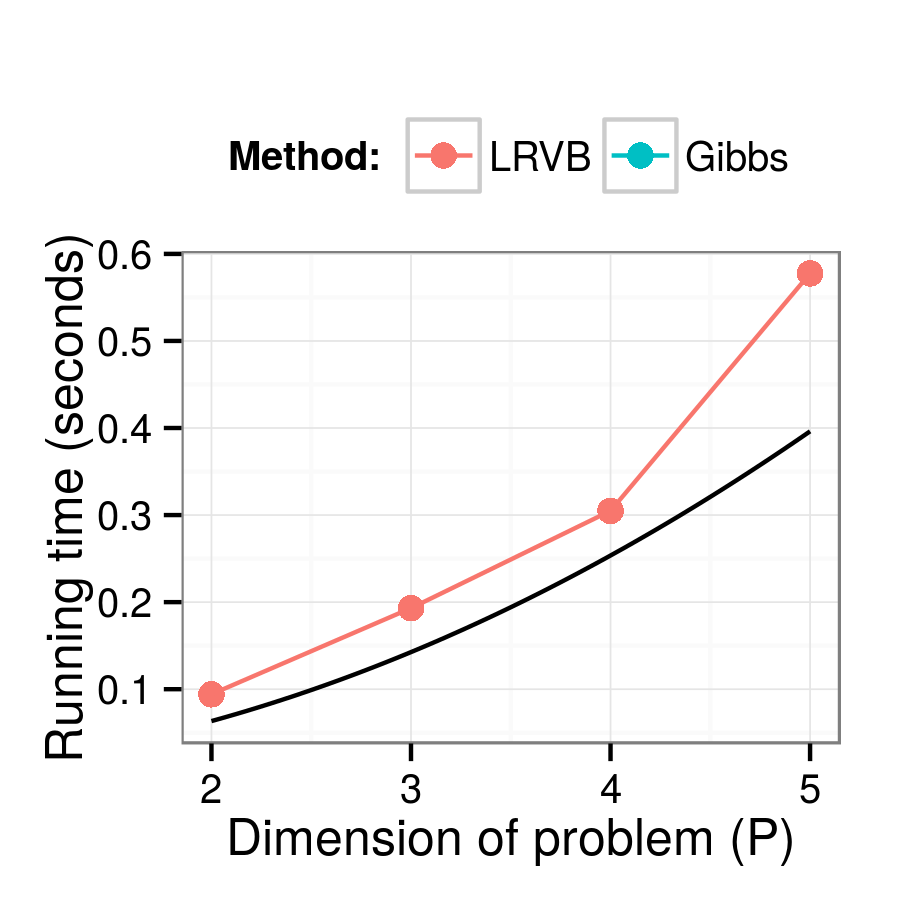
Figure 2: Scaling of LRVB and Gibbs on simulation data in both log and linear scales. Before taking logs, the line in the (N) graph is $y\propto x$, and in the (P) graph, it is $y\propto x^{2}$.

6.5 Influence score experiments

We now demonstrate the accuracy of the influence score formula, Eq. (14), on simulated data and on the MNIST dataset. We first compare Eq. (14) to numeric derivatives. We then look at some patterns in the data that are made visible by having easy-to-calculate influence scores.

6.5.1 Comparison with numeric derivatives

In order verify that LRVB influence scores are correct for this model, we manually perturbed each component of the data and re-fit to find the new MFVB optimum. In other words, we numerically compute the derivative in Eq. (13).

Our simulation used $N=10000$, $P=2$, and $K=2$. This was small enough to calculate the influence score for every data point in every dimension. To select sample data points for MNIST influence scores, we selected $5$ representative data points with different ranges of $\mathbb{E}_{q^{*}}z_{n}$ values so that some had their posterior probability concentrated in only one component, and some that were uncertainly classified between the two components. We then computed the LRVB influence scores from Eq. (14). For comparison, we again manually perturbed each dimension of each data point and re-optimized.

On MNIST, not counting the time to compute the initial LRVB covariance, calculating the LRVB influence scores took $37$ seconds, and the process of perturbing and re-optimizing took $20.7$ minutes.

The comparison between numeric differentiation and LRVB influence scores for both a simulation (left) and MNIST (right) is shown in Fig. (3). The influence scores obtained from the two approaches are practically indistinguishable. Though not shown, in both simulations and on MNIST, for each $\mu$, $\Lambda$, and $\log(\pi)$ parameter, the two methods were as similar to one another as in Fig. (3).

6.5.2 Influence score data

One can see interesting patterns in the data with influence scores. Consider, for example, the simulated data, which is depicted in Fig. (4) and has moderately overlapping components. The graph shows the effect on $\mu_{11}$ of perturbing the $x_{n1}$ (horizontal) coordinate of each datapoint. One can see that the component’s mean is essentially determined by the points that are assigned to it. Interestingly, points on the border between the two components reverse the sign of their effect. This is caused by changes in $\mathbb{E}_{q^{*}}z_{n}$ that more than counterbalance their effects on $\mathbb{E}_{q^{*}}\mu$.

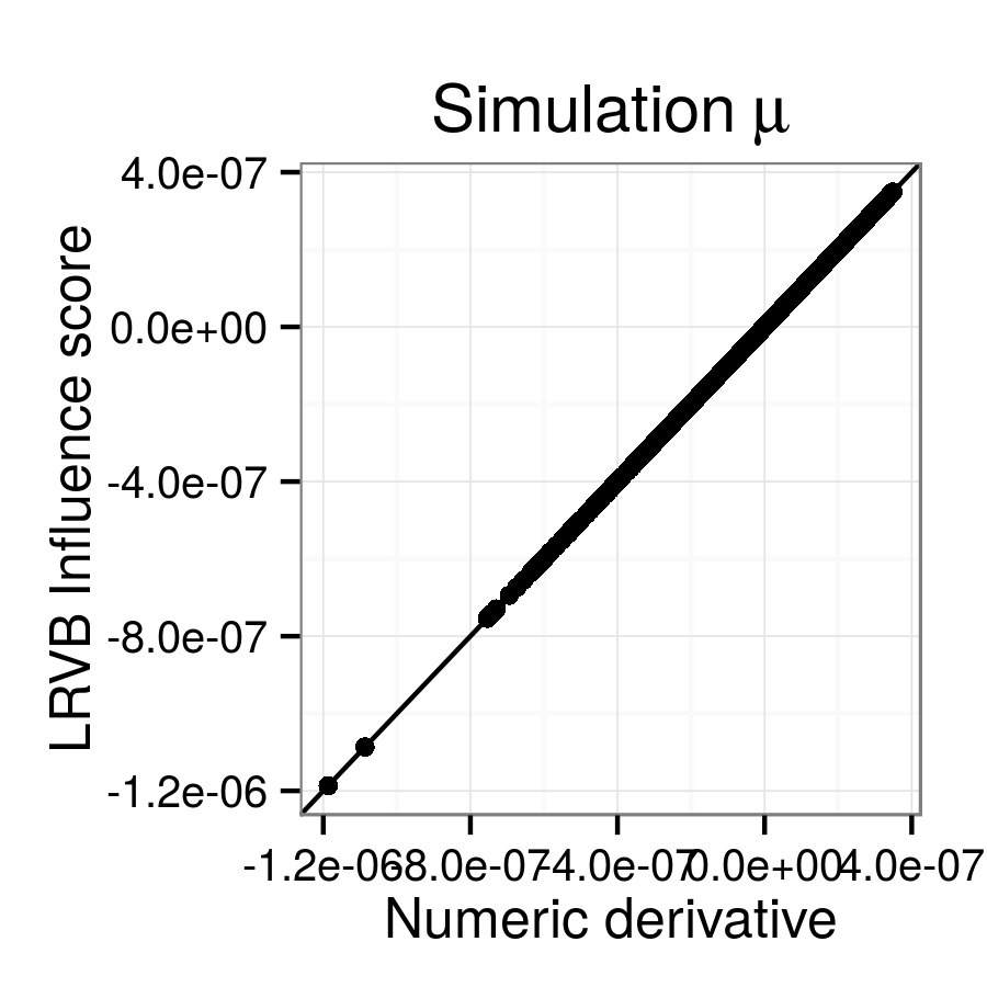
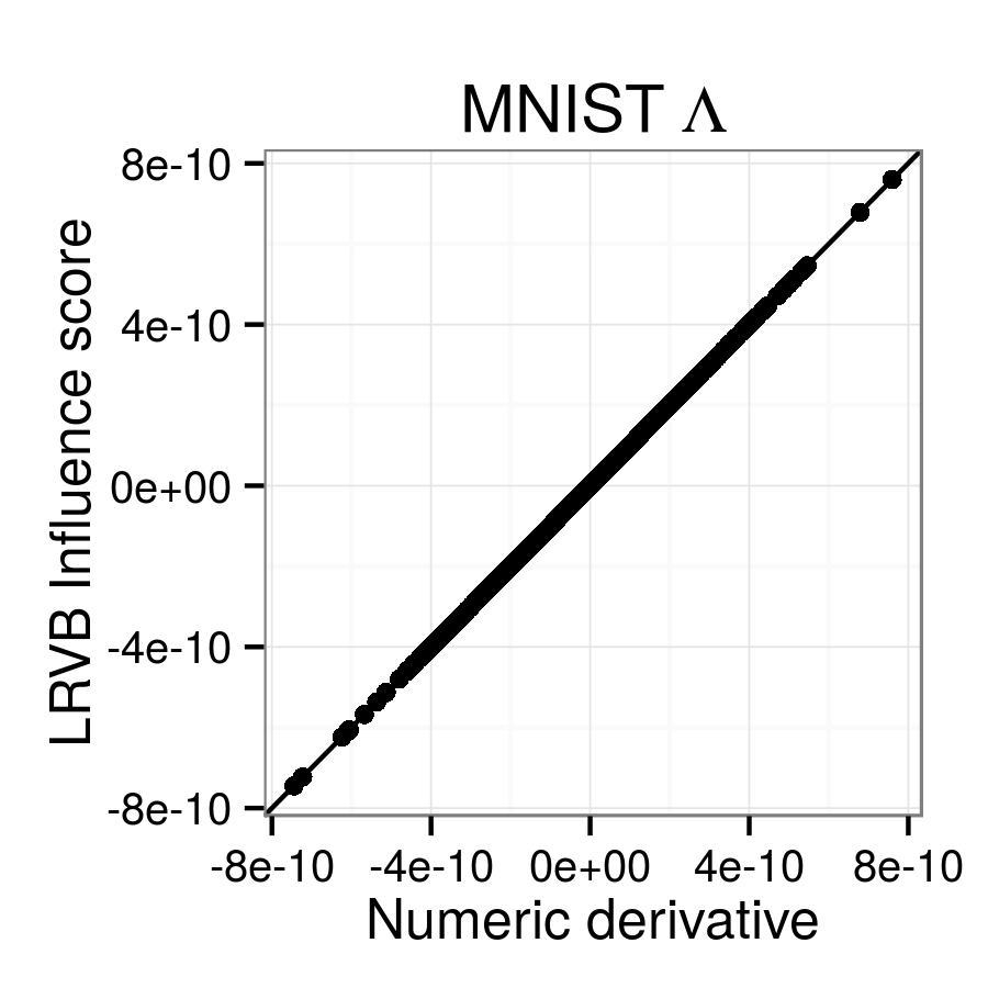
Figure 3: LRVB influence score accuracy. The simulated data uses all $x_{n}$, and the MNIST data uses five representative $x_{n}$.

As can be seen in the simulated data of Fig. (4), the situation becomes more complex when the components overlap even more. Data points that are distant from a component center have nearly as much influence as data points well within the component.

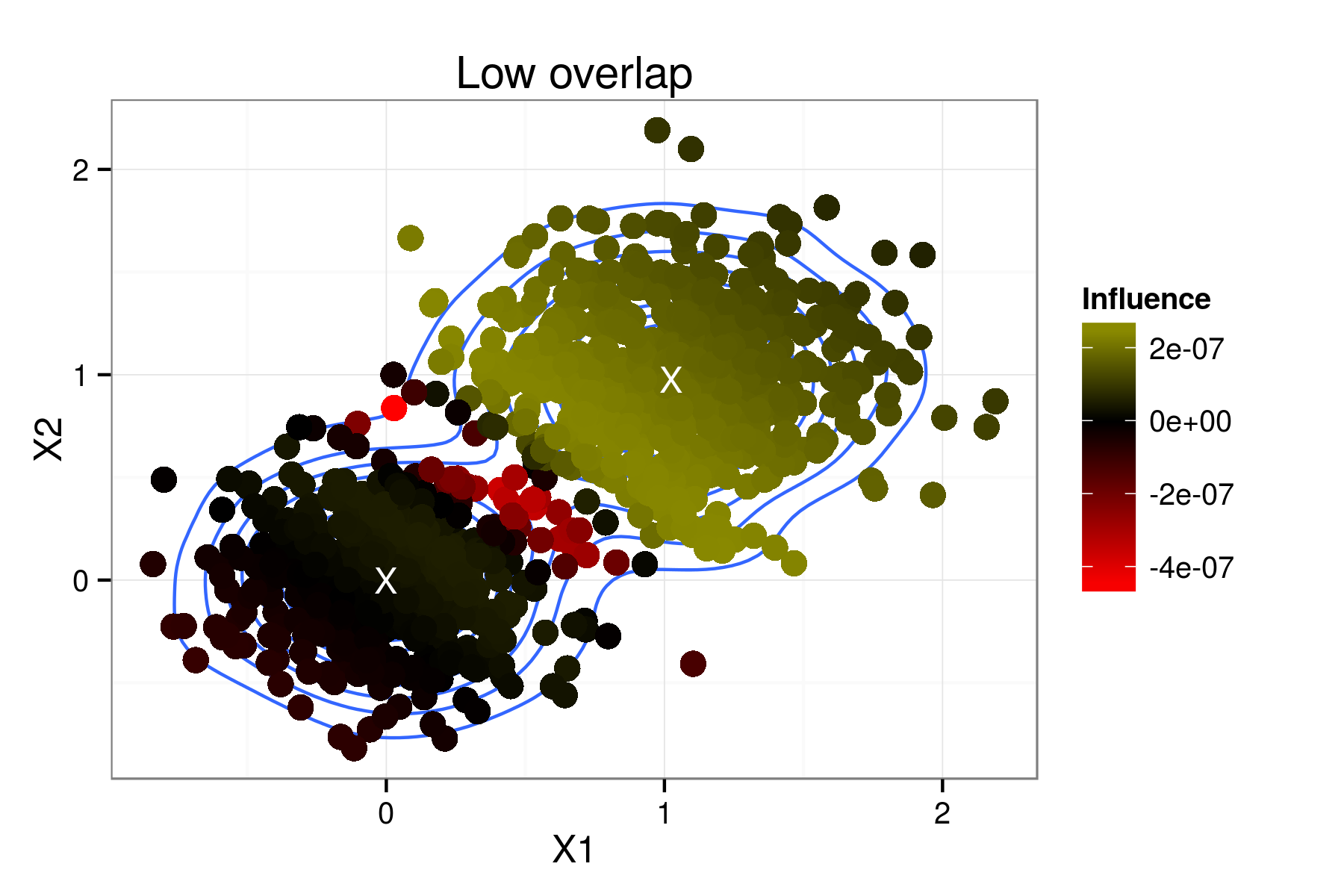
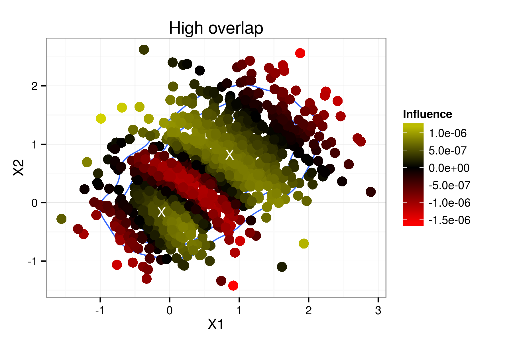
Figure 4: Influence scores for components with different amounts of overlap. Each graph shows the influence of $x_{n1}$ on $\mu_{11}$, which is mean of the upper-right hand component. (X) indicates a component posterior mean.

Finally, we consider influence scores in the MNIST data set. We selected $100$ data points with a 0 or 1 label uniformly at random. In Fig. (4), we considered the influence of one particular dimension of each data point on one particular dimension of each component mean. Recall from Section 6.2 that each data point and component mean is $25$-dimensional. Now we wish to derive a single influence score for the effect of each data point vector-valued $x_{n}$ on each vector-valued component mean $\mu_{k}$.

To that end, we define the influence of a data point $x_{n}$ on $\mu_{k}$ as the directional derivative of $\|\mu_{k}\|_{2}^{2}$ with respect to $x_{n}$. That is, we calculate the vector $\partial\|\mu\|_{2}^{2}/\partial x_{n}$ using LRVB as described above. Then we compute

$$\textrm{Influence of }x_{n}\textrm{ on }\mu_{k}:=\max_{\delta:\|\delta\|=1}\left(\frac{\partial\|\mu_{k}\|_{2}^{2}}{\partial x_{n}^{T}}\delta\right)$$

The resulting influences are plotted in Fig. (5). Each point corresponds to a data point $x_{n}$. Each sub-figure corresponds to a different component mean parameter. The horizontal axis value for point $x_{n}$ is the logit of $\mathbb{E}_{q^{*}}z_{nk}$ (capped at $\pm 15$), which measures the posterior probability that $x_{n}$ came from component $k$.

The two components show very different patterns. Component $0$, the mode with mostly handwritten zeroes, has much higher influence amongst points that are classified within it than component $1$.

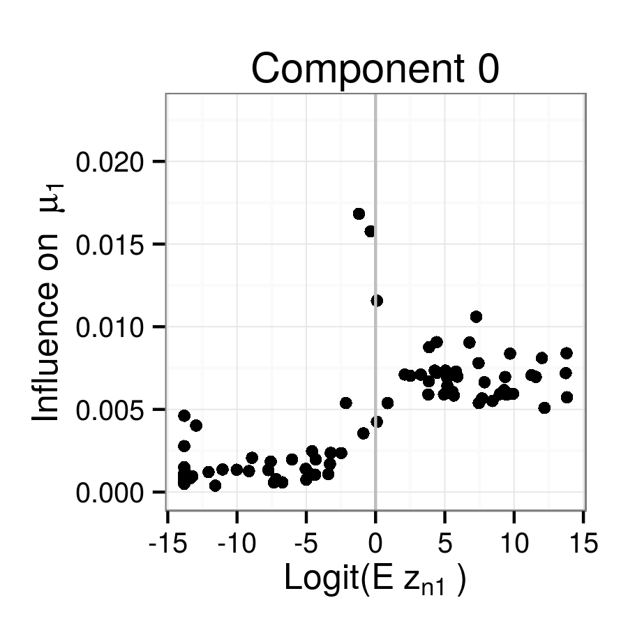
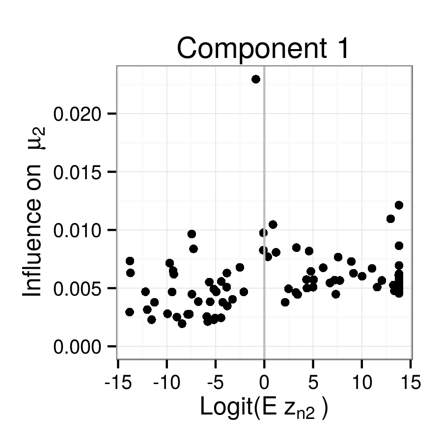
Figure 5: Different influence patterns for the two Gaussians in the MNIST dataset. The 100 data points were chosen randomly. The vertical axis shows the maximum directional derivative of $\mu_{k}$ with respect to changes in the data point, and the horizontal axis shows the (capped) logit posterior probability that the point came from that component.

7 Conclusion

The lack of accurate covariance estimates from the widely used mean-field variational Bayes (MFVB) methodology has been a longstanding shortcoming of MFVB. We have demonstrated that our method, linear response variational Bayes (LRVB), augments MFVB to deliver these covariance estimates in time that scales linearly with the number of data points. We have also shown how to use LRVB to quickly calculate influence scores, a measure of the influence of each data point on posterior parameter means. Our experiments have focused on mixtures of multivariate Gaussians since these have traditionally been used to illustrate the difficulties with MFVB covariance estimation. We hope that in future work our results can be extended to more complex models, including latent Dirichlet allocation and Bayesian nonparametric models, where MFVB has proven its practical success.

Appendix A Derivations

A.1 MFVB for conditional exponential families

First, we require some notation for indexing $\theta$. Recall that the MFVB assumption partitions the components of $\theta$ into $J$ groups according to the factorization

$$q(\theta)=\prod_{j=1}^{J}q_{j}(\theta_{j})=\prod_{j=1}^{J}q(\theta_{j})$$

We follow the common abuse of notation of defining the variational functions through their arguments by writing $q(\theta_{j})$ for $q_{j}(\theta_{j})$.

Each $\theta_{j}$ is be a $D_{j}$-dimensional vector, with $\sum_{j=1}^{J}D_{j}=D$, where the whole $\theta$ vector has dimension $D$. Here and below, we will define the set $[J]:=\{1,...,J\}$.

Let $R(\theta)$ denote a vector of length $\prod_{j\in[J]}(D_{j}+1)$ that is the vector of all possible products of the form $\prod_{j\in[J]}\theta_{ji_{j}}$, where for each $j$, $i_{j}\in\{\emptyset,1,...,D_{j}\}$. That is, $R(\theta)$ is the vector of all possible products of terms of $\theta$ where with at most one term from each $\theta_{j}$, and we define $\theta_{j\emptyset}:=1$. Let $R_{j}(\theta)$ denote the same vector, but excluding terms from $\theta_{j}$, and $R_{jj^{\prime}}(\theta)$ denote the same vector, but excluding both $\theta_{j}$ and $\theta_{j^{\prime}}$.

To aid in intuition, it will sometimes be useful to explicitly write the inner product of $R(\theta)$ with a vector $G$ as a sum of products of components of $\theta_{j}$. Let $G$ be a $|R(\theta)|$-length vector with element $G_{i}$, and let $R(\theta)_{i}$ denote the $i$th row of $R(\theta)$. Then define

$$G^{T}R(\theta)=\sum_{i=1}^{|R(\theta)|}G_{i}R(\theta)_{i}:=\sum_{r\in R}G_{r}\prod_{j\in[J]}\theta_{jr_{j}}$$ (16)

Here, we have “overloaded” the definition of $R$ to express the sum over different products of $\theta$. We define $r_{j}$ as the index of $\theta_{j}$ in the row of $R(\theta)$ corresponding to $r_{j}$, $G_{r}$ as the element of $G$ corresponding to that index set, and the sum over $r\in R$ as the sum over all rows.

We define the inner product of $G$ with $R_{j}(\theta)$ similarly, only with the result as a $D_{j}$-length vector. Specifically, define

$$\sum_{r\in R_{j}}G_{r}\prod_{k\in[J]\setminus j}\theta_{kr_{k}}$$

such that $G_{r}$ is a $D_{j}$-sized column vector. Finally, define

$$\sum_{r\in R_{jj^{\prime}}}G_{r}\prod_{k\in[J]\setminus\{j,j^{\prime}\}}\theta_{kr_{k}}$$

the same way, except where $G_{r}$ is a $D_{j}\times D_{j^{\prime}}$ matrix.

This notation is intended to make it easy to express sums of products of elements of $\theta$ in such a way that no two terms from a single $\theta_{j}$ are multiplied together. The value of this notation will hopefully become clear in the following lemmas.

Lemma A.1.

Suppose Eq. (2) holds across all $j$; that is,

$$p(\theta_{j}|\theta_{i\in[J]\setminus j},x)=\exp(\tilde{\eta}_{j}^{T}\theta_{j}-A_{j}(\tilde{\eta}_{j})).$$

Then the posterior $p(\theta|x)$ can be written in the form

$$\log p(\theta|x)=\sum_{r\in R}G_{r}\prod_{j\in[J]}\theta_{jr_{j}}+C$$ (17)

where the terms $G_{r}$ and $C$ are constant in all $\theta$ .

Proof.

We see that $\log p(\theta|x)=\log p(\theta_{j}|\theta_{i\in[J]\setminus j},x)+\log p(\theta_{i\in[J]\setminus j}|x)$ depends on $\theta_{j}$ only via the first term in the sum. By Eq. (2),

$$p(\theta_{j}|\theta_{i\in[J]\setminus j},x)=\exp(\tilde{\eta}_{j}^{T}\theta_{j}-A_{j}(\tilde{\eta}_{j}))$$

It follows that $\log p(\theta|x)$ is linear in the vector $\theta_{j}$. But this is true for all $\theta_{j}$, and the above form for $p(\theta|x)$ follows. ∎

Lemma A.2.

Suppose Eq. (2) holds across all $j$. Then, for the natural parameter $\tilde{\eta}_{j}$, we have the following equations:

$$\tilde{\eta}_{j} = \sum_{r\in R_{j}}G_{r}\prod_{k\in[J]\setminus j}\theta_{kr_{k}}$$

$$\tilde{\eta}_{j} = \frac{\partial\log p(\theta|x)}{\partial\theta_{j}}$$

$$H = \frac{\partial\eta}{\partial m^{T}}=E_{q^{*}}\left(\frac{\partial^{2}\log p(\theta|x)}{\partial\theta\partial\theta^{T}}\right)$$ (18)

Here, each $G_{r}$ is an $D_{j}$-length vector that is constant with respect to $\theta$.

Proof.

The first result follows by collecting the terms for the $i$th component of $\theta_{j}$ in Eq. (17) and applying Bayes’ theorem. The second is simply observing that differentiating with respect to $\theta_{j}$ is a notationally tidy way to collect the $j$ terms.

For the third result, recall from Eq. (4) that

$$\eta_{j} = \mathbb{E}_{q^{*}}[\tilde{\eta}_{j}]$$

$$= \mathbb{E}_{q^{*}}\left[\sum_{r\in R_{j}}G_{r}\prod_{k\in[J]\setminus j}\theta_{kr_{k}}\right]$$

$$= \sum_{r\in R_{j}}G_{r}\prod_{k\in[J]\setminus j}m_{kr_{k}}\Rightarrow$$

$$\frac{\partial\eta_{j}}{\partial m_{j^{\prime}}^{T}} = \sum_{r\in R_{jj^{\prime}}}G^{\prime}_{r}\prod_{k\in[J]\setminus\{j,j^{\prime}\}}m_{kr_{k}}$$

$$= \mathbb{E}_{q^{*}}\left[\sum_{r\in R_{jj^{\prime}}}G^{\prime}_{r}\prod_{l\in[J]\setminus\{j,j^{\prime}\}}\theta_{kr_{k}}\right]$$

$$= \mathbb{E}_{q^{*}}\left[\frac{\partial\log p(\theta|x)}{\partial\theta_{i}\partial\theta_{j^{\prime}}^{T}}\right]$$

Note that this proof relied on the fact that only one element of $\theta_{j^{\prime}}$ is in each product term, which allowed us to exchange the derivative with respect to the expectation with the expectation of the derivative with respect to $\theta_{j^{\prime}}$.

∎

A.2 Linear response

We here derive the three equalities in Eqs. (7), (8), and (9), which appear respectively as three propositions below. In these propositions, we assume that $p(\theta|x)$ is in the exponential family as above. We will further assume that all natural parameters (for $p$ or variational approximations) are in the interior of the parameter space. The fact that the natural parameters are on the interior of the feasible space means that there exists an open ball around them that is also feasible. Let that ball have radius $\delta$, and let $t$ be within a $\delta$ ball of the origin. Then $p_{t}(\theta|x)$ is well defined for $t$ in an open set containing zero. These assumptions will allow us to apply dominated convergence (cf. Section 2.3 of [23]).

Proposition A.3.

$\frac{d}{dt}\mathbb{E}_{p_{t}}\theta=\Sigma_{t}$.

Proof.

$$\frac{d}{dt^{T}}\mathbb{E}_{p_{t}}\theta =\frac{d}{dt^{T}}\int_{\theta}\theta e^{t^{T}\theta-c(t)}p(\theta|x)d\theta\quad\textrm{by the definition of $p_{t}$ in Eq.~{}(\ref{eq:perturbed_dens})}$$

$$=\int_{\theta}\theta\left[\frac{d}{dt^{T}}e^{t^{T}\theta-c(t)}\right]p(\theta|x)d\theta\quad\textrm{by dominated convergence}$$

$$=\int_{\theta}\theta\theta^{T}e^{t^{T}\theta-c(t)}p(\theta|x)d\theta-\int_{\theta}\theta e^{t^{T}\theta-c(t)}p(\theta|x)d\theta\cdot\frac{dc(t)}{dt^{T}}$$

$$=\mathbb{E}_{p_{t}}\left[\theta\theta^{T}\right]-\mathbb{E}_{p_{t}}\left[\theta\right]\mathbb{E}_{p_{t}}\left[\theta\right]^{T}=\Sigma_{t}$$

∎

To approximate $\frac{dm_{t}}{dt^{T}}$, we assume not only that $m_{t}\approx\mathbb{E}_{p_{t}}\theta$ for any particular $t$ but further that $m_{t}$ tracks the true mean $\mathbb{E}_{p_{t}}\theta$ as $t$ varies. In this case, by Proposition A.3, we have

$$\frac{dm_{t}}{dt^{T}}\approx\frac{d}{dt^{T}}\mathbb{E}_{p_{t}}\theta=\Sigma_{t},$$

the first (approximate) equality in Eq. (7).

To derive the final two equalities in Eqs. (8) and (9), we make use of the following lemma.

Lemma A.4.

$M_{t,j}$ depends on $t$ only via $\eta_{t,j}$, the natural parameter of the $q_{t,j}^{*}$ distribution. And $\frac{dM_{t,j}}{d\eta_{t,j}^{T}}=\Sigma_{q_{t,j}^{*}}$.

Proof.

The first part of the lemma follows from writing the definition of $M_{t,j}$:

$$M_{t,j}=\mathbb{E}_{q_{t,j}^{*}}\theta_{j}=\int_{\theta_{j}}\theta_{j}\exp\left(\eta_{t,j}^{T}\theta_{j}-A_{j}\left(\eta_{t,j}\right)\right)d\theta_{j}.$$

For the second part,

$$\frac{dM_{t,j}}{d\eta_{t,j}^{T}} =\int_{\theta_{j}}\frac{d}{d\eta_{t,j}^{T}}\theta_{j}\exp\left(\eta_{t,j}^{T}\theta_{j}-A_{j}\left(\eta_{t,j}\right)\right)d\theta_{j}\quad\textrm{by dominated convergence}$$

$$=\int_{\theta_{j}}\theta_{j}\left[\theta_{j}^{T}-\mathbb{E}_{q_{t,j}^{*}}\theta_{j}^{T}\right]\exp\left(\eta_{t,j}^{T}\theta_{j}-A_{j}\left(\eta_{t,j}\right)\right)d\theta_{j}$$

$$=\Sigma_{q_{t,j}^{*}}$$

∎

Proposition A.5.

$\frac{\partial M_{t}}{\partial t^{T}}=V_{t}.$

Proof.

By Lemma A.4, we have for any indices $i$ and $j$ in $[J]$ that

$$\frac{\partial M_{t,j}}{\partial t_{i}^{T}}=\frac{dM_{t,j}}{d\eta_{t,j}^{T}}\frac{\partial\eta_{t,j}}{\partial t_{i}^{T}},$$ (19)

where the first factor is also given by Lemma A.4. It remains to find the second factor, $\frac{\partial\eta_{t,j}}{\partial t_{i}^{T}}$. By the discussion after Eq. (2) and the construction of $p_{t}$, the natural parameter $\tilde{\eta}_{t,j}$ of $p_{t}\left(\theta_{j}|\theta_{i\in[J]\setminus j},x\right)$ satisfies

$$\tilde{\eta}_{t,j}=\sum_{r\in R_{j}}G_{r}\prod_{k\in[J]\setminus j}\theta_{kr_{k}}+t_{j}.$$

So, as in the derivation of Eq. (4), the natural parameter $\eta_{t,j}$ of $q_{j}^{*}(\theta_{j})$ satisfies

$$\eta_{t,ji}=\sum_{r\in R_{j}}G_{r}\prod_{k\in[J]\setminus j}m_{t,kr_{k}}+t_{j}$$ (20)

for $m_{t,r}:=\mathbb{E}_{q^{*}_{t,r}}\theta_{r}$.

Let $d_{j}$ be the dimension of $\theta_{j}$ and hence the dimension of $\eta_{t,j}$ and $t_{j}$. Hence,

$$\frac{\partial\eta_{t,j}}{\partial t_{i}^{T}}=\left\{\begin{array}[]{ll}I_{d_{j}}&j=i\\ 0_{d_{j},d_{i}}&\mathrm{else}\end{array}\right.,$$

where $I_{a}$ is the identity matrix of dimension $a$, and $0_{a,b}$ is the all zeros matrix of dimension $a\times b$.

Finally, by Eq. (19), Lemma A.4, and the expression for $\frac{\partial\eta_{t,j}}{\partial t_{i}^{T}}$ just obtained, we have

$$\frac{\partial M_{t}}{\partial t^{T}}=V_{t}I_{D}=V_{t}.$$

∎

Proposition A.6.

$\frac{dM_{t}}{dm_{t}^{T}}=V_{t}\frac{\partial\eta_{t}}{\partial m_{t}^{T}}.$

Proof.

By Lemma A.4 and analogous to Eq. (19), we have

$$\frac{\partial M_{t,j}}{\partial m_{t,i}^{T}}=\frac{dM_{t,j}}{d\eta_{t,j}^{T}}\frac{\partial\eta_{t,j}}{\partial m_{t,i}^{T}}.$$ (21)

The result follows immediately from Lemma A.4. ∎

Appendix B Multivariate normal posteriors and SEM

For any target distribution $p(\theta|x)$, it is well-known that MFVB cannot be used to estimate the covariances between the components of $\theta$. In particular, if $q^{*}$ is the estimate of $p(\theta|x)$ returned by MFVB, $q^{*}$ will have a block-diagonal covariance matrix—no matter the form of the covariance of $p(\theta|x)$. By contrast, the next result shows that the LRVB covariance estimate is exactly correct in the case where the target distribution, $p(\theta|x)$, is (multivariate) normal.

In order to prove this result, we will rely on the following lemma.

Lemma B.1.

Consider a target posterior distribution characterized by $p(\theta|x)=\mathcal{N}(\theta|\mu,\Sigma)$, where $\mu$ and $\Sigma$ may depend on $x$, and $\Sigma$ is invertible. Let $\theta=(\theta_{1},\ldots,\theta_{J})$, and consider a MFVB approximation to $p(\theta|x)$ that factorizes as $q(\theta)=\prod_{j}q(\theta_{j})$. Then the variational posterior means are the true posterior means; i.e. $m_{j}=\mu_{j}$ for all $j$ between $1$ and $J$.

Proof.

The derivation of MFVB for the multivariate normal can be found in Section 10.1.2 of [5]; we highlight some key results here. Let $\Lambda=\Sigma^{-1}$. Let the $j$ index on a row or column correspond to $\theta_{j}$, and let the $-j$ index correspond to $\{\theta_{i}:i\in[J]\setminus j\}$. E.g., for $j=1$,

$$\Lambda=\left[\begin{array}[]{ll}\Lambda_{11}&\Lambda_{1,-1}\\ \Lambda_{-1,1}&\Lambda_{-1,-1}\end{array}\right].$$

By the assumption that $p(\theta|x)=\mathcal{N}(\theta|\mu,\Sigma)$, we have

$$\log p(\theta_{j}|\theta_{i\in[J]\setminus j},x)=-\frac{1}{2}(\theta_{j}-\mu_{j})^{T}\Lambda_{jj}(\theta_{j}-\mu_{j})+(\theta_{j}-\mu_{j})^{T}\Lambda_{j,-j}(\theta_{-j}-\mu_{-j})+C,$$ (22)

where the final term is constant with respect to $\theta_{j}$. It follows that

$$\log q^{*}_{j}(\theta_{j}) =\mathbb{E}_{q^{*}_{i}:i\in[J]\setminus j}\log p(\theta,x)+C$$

$$=-\frac{1}{2}\theta_{j}^{T}\Lambda_{jj}\theta_{j}+\theta_{j}\mu_{j}\Lambda_{jj}-\theta_{j}\Lambda_{j,-j}(\mathbb{E}_{q^{*}}\theta_{-j}-\mu_{-j}).$$

So

$$q^{*}_{j}(\theta_{j})=\mathcal{N}(\theta_{j}|m_{j},\Lambda_{jj}^{-1}),$$

with mean parameters

$$m_{j}=\mathbb{E}_{q^{*}_{j}}\theta_{j}=\mu_{j}-\Lambda_{jj}^{-1}\Lambda_{j,-j}(m_{-j}-\mu_{-j})$$ (23)

as well as an equation for $\mathbb{E}_{q^{*}}\theta^{T}\theta$.

Note that $\Lambda_{jj}$ must be invertible, for if it were not, $\Sigma$ would not be invertible.

The solution $m=\mu$ is a unique stable point for Eq. (23), since the fixed point equations for each $j$ can be stacked and rearranged to give

$$m-\mu = -\left[\begin{array}[]{ccccc}0&\Lambda_{11}^{-1}\Lambda_{12}&\cdots&\Lambda_{11}^{-1}\Lambda_{1\left(J-1\right)}&\Lambda_{11}^{-1}\Lambda_{1J}\\ \vdots&&\ddots&&\vdots\\ \Lambda_{JJ}^{-1}\Lambda_{J1}&\Lambda_{JJ}^{-1}\Lambda_{J2}&\cdots&\Lambda_{JJ}^{-1}\Lambda_{J\left(J-1\right)}&0\end{array}\right]\left(m-\mu\right)$$

$$= -\left[\begin{array}[]{ccccc}\Lambda_{11}^{-1}&\cdots&0&\cdots&0\\ \vdots&\ddots&&&\vdots\\ 0&&\ddots&&0\\ \vdots&&&\ddots&\vdots\\ 0&\cdots&0&\cdots&\Lambda_{JJ}^{-1}\end{array}\right]\left[\begin{array}[]{ccccc}0&\Lambda_{12}&\cdots&\Lambda_{1\left(J-1\right)}&\Lambda_{1J}\\ \vdots&&\ddots&&\vdots\\ \Lambda_{J1}&\Lambda_{J2}&\cdots&\Lambda_{J\left(J-1\right)}&0\end{array}\right]\left(m-\mu\right)\Leftrightarrow$$

$$0 = \left[\begin{array}[]{ccccc}\Lambda_{11}&\cdots&0&\cdots&0\\ \vdots&\ddots&&&\vdots\\ 0&&\ddots&&0\\ \vdots&&&\ddots&\vdots\\ 0&\cdots&0&\cdots&\Lambda_{JJ}\end{array}\right]\left(m-\mu\right)+$$

$$\left[\begin{array}[]{ccccc}0&\Lambda_{12}&\cdots&\Lambda_{1\left(J-1\right)}&\Lambda_{1J}\\ \vdots&&\ddots&&\vdots\\ \Lambda_{J1}&\Lambda_{J2}&\cdots&\Lambda_{J\left(J-1\right)}&0\end{array}\right]\left(m-\mu\right)\Leftrightarrow$$

$$0 = \Lambda\left(m-\mu\right)\Leftrightarrow$$

$$m = \mu.$$

The last step follows from the assumption that $\Sigma$ (and hence $\Lambda$) is invertible. It follows that $\mu$ is the unique stable point of Eq. (23).

∎

Proposition B.2.

Assume we are in the setting of Lemma B.1, where additionally $\mu$ and $\Sigma$ are on the interior of the feasible parameter space. Then the LRVB covariance estimate exactly captures the true covariance, $\hat{\Sigma}=\Sigma$.

Proof.

Consider the perturbation for LRVB defined in Eq. (5). By perturbing the log likelihood, we change both the true means $\mu_{t}$ and the variational solutions, $m_{t}$. The result is a valid density function since the original $\mu$ and $\Sigma$ are on the interior of the parameter space. By Lemma B.1, the MFVB solutions are exactly the true means, so $m_{t,j}=\mu_{t,j}$, and the derivatives are the same as well. This means that the first term in Eq. (10) is not approximate, i.e.

$$\frac{dm_{t}}{dt^{T}}=\frac{d}{dt^{T}}\mathbb{E}_{p_{t}}\theta=\Sigma_{t},$$

It follows from the arguments in Appendix B that the LRVB covariance matrix is exact, and $\hat{\Sigma}=\Sigma$.

∎

B.1 Comparison with supplemented expectation-maximization

This result about the multivariate normal distribution draws a connection between LRVB corrections and the “supplemented expectation-maximization” (SEM) method of [13]. SEM is an asymptotically exact covariance correction for the EM algorithm that transforms the full-data Fisher information matrix into the observed-data Fisher information matrix using a correction that is formally similar to Eq. (10). In this section, we argue that this similarity is not a coincidence; in fact the SEM correction is an asymptotic version of LRVB with two variational blocks, one for the missing data and one for the unknown parameters.

Although LRVB as described here requires a prior (unlike SEM, which supplements the MLE), the two covariance corrections coincide when the full information likelihood is approximately log quadratic and proportional to the posterior, $p(\theta|x)$. This might be expected to occur when we have a large number of independent data points informing each parameter—i.e., when a central limit theorem applies and the priors do not affect the posterior. In the full information likelihood, some terms may be viewed as missing data, whereas in the Bayesian model the same terms may be viewed as latent parameters, but this does not prevent us from formally comparing the two methods.

We can draw a term-by-term analogy with the equations in [13]. We denote variables from the SEM paper with a superscript “$SEM$” to avoid confusion. MFVB does not differentiate between missing data and parameters to be estimated, so our $\theta$ corresponds to $(\theta^{SEM},Y_{mis}^{SEM})$ in [13]. SEM is an asymptotic theory, so we may assume that $(\theta^{SEM},Y_{mis}^{SEM})$ have a multivariate normal distribution, and that we are interested in the mean and covariance of $\theta^{SEM}$.

In the E-step of [13], we replace $Y_{mis}^{SEM}$ with its conditional expectation given the data and other $\theta^{SEM}$. This corresponds precisely to Eq. (23), taking $\theta_{j}=Y_{mis}^{SEM}$. In the M-step, we find the maximum of the log likelihood with respect to $\theta^{SEM}$, keeping $Y_{mis}^{SEM}$ fixed at its expectation. Since the mode of a multivariate normal distribution is also its mean, this, too, corresponds to Eq. (23), now taking $\theta_{j}=\theta^{SEM}$.

It follows that the MFVB and EM fixed point equations are the same; i.e., our $M$ is the same as their $M^{SEM}$, and our $\partial M/\partial m$ of Eq. (21) corresponds to the transpose of their $DM^{SEM}$, defined in Eq. (2.2.1) of [13]. Since the “complete information” corresponds to the variance of $\theta^{SEM}$ with fixed values for $Y_{OBS}^{SEM}$, this is the same as our $\Sigma_{q^{*},11}$, the variational covariance, whose inverse is $I_{oc}^{-1}$. Taken all together, this means that equation (2.4.6) of [13] can be re-written as our Eq. (10).

$$V^{SEM}= I_{oc}^{-1}\left(I-DM^{SEM}\right)^{-1}\Rightarrow$$

$$\Sigma= V\left(I-\left(\frac{\partial M}{\partial m^{T}}\right)^{T}\right)^{-1}=\left(I-\frac{\partial M}{\partial m^{T}}\right)^{-1}V$$

Appendix C Multivariate normal mixture details

In this section we derive the basic formulas needed to calculate Eq. (10) and Eq. (14) for a finite mixture of normals, which is the model used in Section 6. We will follow the notation introduced in Section 6.1.

Let each observation, $x_{n}$, be a $P\times 1$ vector. We will denote the $P$th component of the $n$th observation $x_{n}$, with a similar pattern for $z$ and $\mu$. We will denote the $p$, $q$th entry in the matrix $\Lambda_{k}$ as $\Lambda_{k,pq}$. The data generating process is as follows:

$$\log P\left(x_{n}|z_{n},\mu,\Lambda\right) = \sum_{n=1}^{N}z_{nk}\log\phi_{k}(x_{n})+C$$

$$\log\phi_{k}(x) = -\frac{1}{2}\left(x-\mu_{k}\right)^{T}\Lambda_{k}\left(x-\mu_{k}\right)+\frac{1}{2}\log\left|\Lambda_{k}\right|+C$$

$$\log P(z_{nk}|\pi_{k}) = \sum_{k=1}^{K}z_{nk}\log\pi_{k}+C$$

$$\log P(z,\mu,\pi,\Lambda|x) = \sum_{n=1}^{N}\sum_{k=1}^{K}z_{nk}\left(\log\pi_{k}-\frac{1}{2}\left(x_{n}-\mu_{k}\right)^{T}\Lambda_{k}\left(x_{n}-\mu_{k}\right)+\frac{1}{2}\log\left|\Lambda_{k}\right|\right)+C$$

In all our results we simply used improper, flat priors, though it would be trivial to incorporate conjugate priors.

From the assumptions in Eq. (5), the posterior expectation of $x^{*}$ will always have $\mathbb{E}_{q}x^{*}=x$, so for notational convenience we can simply drop the $*$ and apply the LRVB formulas as if $x$ were a random parameter. However, it is useful to remember that the parameter $x$ is different from the variable we condition on – we are actually estimating $p(\alpha,z,x^{*}|x)$.

The parameters $\mu_{k}$, $\Lambda_{k}$, $\pi$, and $z_{n}$ will each be given their own variational distribution. By standard results, the variational distributions will be:

$$q_{\mu_{k}} =$$ Multivariate Normal

$$q_{\Lambda_{k}} =$$ Wishart

$$q_{\pi} =$$ Dirichlet

$$q_{z_{n}} =$$ Multinoulli (one multinomial draw)

$$q_{x^{*}_{n}} =$$ Multivariate Normal

The sufficient statistics for $\mu_{k}$ are all terms of the form $\mu_{kp}$ and $\mu_{kp}\mu_{kq}$. Consequently, the sub-vector of $\theta$ corresponding to $\mu_{k}$ is

$$\theta_{\mu_{k}} = \left(\begin{array}[]{c}\mu_{k1}\\ \vdots\\ \mu_{kp}\\ \mu_{k1}\mu_{k1}\\ \mu_{k1}\mu_{k2}\\ \vdots\\ \mu_{kP}\mu_{kP}\end{array}\right)$$

We will only save one copy of $\mu_{kp}\mu_{kq}$ and $\mu_{kq}\mu_{kp}$, so $\theta_{\mu_{k}}$ has length $P+\frac{1}{2}\left(P+1\right)P$. For all the parameters, we denote the complete stacked vector without a $k$ subscript:

$$\theta_{\mu} = \left(\begin{array}[]{c}\theta_{\mu_{1}}\\ \vdots\\ \theta_{\mu_{K}}\end{array}\right)$$

The sufficient statistics for $x^{*}$ are analogous to those for $\mu$.

The sufficient statistics for $\Lambda_{k}$ are all the terms $\Lambda_{k,pq}$ and the term $\log\left|\Lambda_{k}\right|$. Again, since $\Lambda$ is symmetric, we do not keep redundant terms, so $\theta_{\Lambda_{k}}$ has length $1+\frac{1}{2}\left(P+1\right)P$.

The sufficient statistics for $\pi$ is the $K$-vector $\left(\log\pi_{1},...,\log\pi_{K}\right)$.

The sufficient statistics for $z$ is simply the $N\times K$ values $z_{nk}$ themselves.

In terms of Section 5, we have

$$\alpha = \left(\begin{array}[]{c}\theta_{\mu}\\ \theta_{\Lambda}\\ \theta_{\pi}\end{array}\right)$$

$$z = \left(\begin{array}[]{c}\theta_{z}\end{array}\right)$$

$$x = \left(\theta_{x}\right)$$

That is, we are primarily interested in the covariance of the sufficient statistics of $\mu$, $\Lambda$, and $\pi$, $z$ are nuisance parameters, and $x^{*}$ is the “unobserved” data.

To put the log likelihood in terms useful for LRVB, we must express it in terms of the sufficient statistics, taking into account the fact the $\theta$ vector does not store redundant terms (e.g. it will only keep $\Lambda_{ab}$ for $a<b$ since $\Lambda$ is symmetric).

$$-\frac{1}{2}\left(x_{n}-\mu_{k}\right)^{T}\Lambda_{k}\left(x_{n}-\mu_{k}\right) = -\frac{1}{2}trace\left(\Lambda_{k}\left(x_{n}-\mu_{k}\right)\left(x_{n}-\mu_{k}\right)^{T}\right)$$

$$= -\frac{1}{2}\sum_{a}\sum_{b}\left(\Lambda_{k,ab}\left(x_{n,a}-\mu_{k,a}\right)\left(x_{n,b}-\mu_{k,b}\right)\right)$$

$$= -\frac{1}{2}\sum_{a}\sum_{b}\left(\Lambda_{k,ab}\mu_{k,a}\mu_{k,b}-\Lambda_{k,ab}x_{n,a}\mu_{k,b}-\Lambda_{k,ab}x_{n,b}\mu_{k,a}+\Lambda_{k,ab}x_{n,a}x_{n,b}\right)$$

$$= -\frac{1}{2}\sum_{a}\Lambda_{k,aa}\left(\mu_{k}^{2}\right)^{a}+\sum_{a}\Lambda_{k,aa}x_{n,a}\mu_{k,a}-\frac{1}{2}\sum_{a}\Lambda_{k,aa}\left(x_{n}^{2}\right)^{2}-$$

$$\frac{1}{2}\sum_{a\neq b}\Lambda_{k,ab}\mu_{k,a}\mu_{k,b}+\sum_{a\neq b}\Lambda_{k,ab}x_{n,a}\mu_{k,b}-\frac{1}{2}\sum_{a\neq b}\Lambda_{k,ab}x_{n,a}x_{n,b}$$

$$= -\frac{1}{2}\sum_{a}\Lambda_{k,aa}\left(\mu_{k}^{2}\right)^{a}+\sum_{a}\Lambda_{k,aa}x_{n,a}\mu_{k,a}-\frac{1}{2}\sum_{a}\Lambda_{k,aa}\left(x_{n}^{2}\right)^{2}-$$

$$\sum_{a<b}\Lambda_{k,ab}\mu_{k,a}\mu_{k,b}+\sum_{a<b}\Lambda_{k,ab}\left(x_{n,a}\mu_{k,b}+x_{n,b}\mu_{k,a}\right)-\sum_{a<b}\Lambda_{k,ab}x_{n,a}x_{n,b}$$

The MFVB updates and covariances in $V$ are all given by properties of standard distributions. To compute the LRVB corrections, it only remains to calculate the hessian of $H$. These terms can be read directly off the posterior. First we calculate derivatives with respect to components of $\mu$.

$$\frac{\partial^{2}H}{\partial\mu_{k,a}\partial\Lambda_{k,ab}} = \sum_{i}z_{nk}x_{n,b}$$

$$\frac{\partial^{2}H}{\partial\left(\mu_{k,a}\mu_{k,b}\right)\partial\Lambda_{k,ab}} = -\left(\frac{1}{2}\right)^{1(a=b)}\sum_{n}z_{nk}$$

$$\frac{\partial^{2}H}{\partial\mu_{k,a}\partial z_{nk}} = \sum_{b}\Lambda_{k,ab}x_{n,b}$$

$$\frac{\partial^{2}H}{\partial\left(\mu_{k,a}\mu_{k,b}\right)\partial z_{nk}} = -\left(\frac{1}{2}\right)^{1(a=b)}\Lambda_{k,ab}$$

All other $\mu$ derivatives are zero. For $\Lambda$,

$$\frac{\partial^{2}H}{\partial\Lambda_{k,ab}\partial z_{nk}} = -\left(\frac{1}{2}\right)^{1(a=b)}\left(x_{n,a}x_{n,b}-\mu_{k,a}x_{n,b}-\mu_{k,b}x_{n,a}+\mu_{k,a}\mu_{k,b}\right)$$

$$\frac{\partial^{2}H}{\partial\log\left|\Lambda_{k}\right|\partial z_{nk}} = \frac{1}{2}$$

The remaining $\Lambda$ derivatives are zero. The only nonzero second derivatives for $\log\pi$ are to $Z$ and are given by

$$\frac{\partial^{2}H}{\partial\log\pi_{j}\partial z_{nk}} = 1$$

To calculate the influence scores, we additionally need second derivatives involving $x$.

$$\frac{\partial^{2}H}{\partial x_{n,a}\partial\mu_{k,b}} = z_{nk}\Lambda_{k,ab}$$

$$\frac{\partial^{2}H}{\partial x_{n,a}\partial\Lambda_{k,ab}} = z_{nk}\mu_{k,b}$$

$$\frac{\partial^{2}H}{\partial x_{n,a}\partial z_{nk}} = \sum_{b}\mu_{k,b}\Lambda_{k,ab}$$

$$\frac{\partial^{2}H}{\partial\left(x_{n,a}x_{n,b}\right)\partial\Lambda_{k,ab}} = -z_{nk}\left(\frac{1}{2}\right)^{1\left(a=b\right)}$$

$$\frac{\partial^{2}H}{\partial\left(x_{n,a}x_{n,b}\right)\partial z_{nk}} = -\Lambda_{k,ab}\left(\frac{1}{2}\right)^{1(a=b)}$$

All other second derivatives involving $x$ are zero. Note in particular that $H_{zz}=0$, allowing efficient calculation of Eq. (11).

Appendix D Influence scores

D.1 Influence score derivations

In this section, we derive the formulas in Section 5. We will follow the notation there defined. Consider the “influence score” given by the derivative of the conditional expectation:

$$m_{\theta_{i}}\left(x_{n}\right) = \mathbb{E}_{p}\left[\theta_{i}|x_{1},...,x_{n},...,x_{N}\right]$$

$$\frac{d}{dx_{n}}m_{\theta_{i}}\left(x_{n}\right) := m_{\theta_{i}}^{\prime}\left(x_{n}\right)$$

A Taylor expansion of $m_{\theta_{i}}\left(x^{*}_{n}\right)$ around $x_{n}$ gives

$$m_{\theta_{i}}\left(x_{n}^{*}\right) = m_{\theta_{i}}\left(x_{n}\right)+m_{\theta_{i}}^{\prime}\left(x_{n}\right)\left(x_{n}^{*}-x_{n}\right)+$$

$$\quad\quad O\left(\left(x_{n}^{*}-x_{n}\right)^{2}\right)$$

Multiplying both sides by $\left(x_{n}^{*}-x_{n}\right)$ and taking expectations conditional on $x$ gives

$$\mathbb{E}\left[\left(m_{\theta_{i}}\left(x_{n}^{*}\right)-m_{\theta_{i}}\left(x_{n}\right)\right)\left(x_{n}^{*}-x_{n}\right)|x\right]$$

$$\quad=m_{\theta_{i}}^{\prime}\left(\theta_{i},x_{n}\right)\mathbb{E}\left[\left(x_{n}^{*}-x_{n}\right)^{2}|x\right]+O\left(\left(x_{n}^{*}-x_{n}\right)^{3}\right)$$

On the left side,

$$\mathbb{E}\left[\left(m_{\theta_{i}}\left(x_{n}^{*}\right)-m_{\theta_{i}}\left(x_{n}\right)\right)\left(x_{n}^{*}-x_{n}\right)|x\right]$$

$$\quad=\mathbb{E}\left[\mathbb{E}\left[\left(m_{\theta_{i}}\left(x_{n}^{*}\right)-m_{\theta_{i}}\left(x_{n}\right)\right)\left(x_{n}^{*}-x_{n}\right)|x_{n}^{*}\right]|x\right]$$

$$\quad=\mathbb{E}\left[\mathbb{E}\left[\left(\mathbb{E}\left[\theta_{i}|x_{1},.,x_{n}^{*},.,x_{N}\right]-m_{\theta_{i}}\left(x_{n}\right)\right)\left(x_{n}^{*}-x_{n}\right)|x_{n}^{*}\right]|x\right]$$

$$\quad=\mathbb{E}\left[\mathbb{E}\left[\left(\theta_{i}-m_{\theta_{i}}\left(x_{n}\right)\right)\left(x_{n}^{*}-x_{n}\right)|x_{n}^{*}\right]|x\right]$$

$$\quad=\mathbb{E}\left[\left(\theta_{i}-m_{\theta_{i}}\left(x_{n}\right)\right)\left(x_{n}^{*}-x_{n}\right)|x\right]$$

$$\quad=Cov\left(\theta_{i},x_{n}^{*}|x\right)$$

On the right side,

$$m_{\theta_{i}}^{\prime}\left(\theta_{i},x_{n}\right)\mathbb{E}\left[\left(x_{n}^{*}-x_{n}\right)^{2}|x\right]+O\left(\left(x_{n}^{*}-x_{n}\right)^{3}\right)$$

$$\quad=m_{\theta_{i}}^{\prime}\left(\theta_{i},x_{n}\right)\epsilon+O\left(\epsilon^{\frac{3}{2}}\right)$$

So that

$$m_{\theta_{i}}^{\prime}\left(\theta_{i},x_{n}\right) = \frac{1}{\epsilon}Cov\left(\theta_{i},x_{n}^{*}|x\right)+O\left(\epsilon^{\frac{3}{2}}\right)$$

…which is Eq. (13).

We now assume that our parameter space can be divided into types of variables: $\alpha$ and $z$ as before, and $x$, the perturbed data. As before, we also assume that each has its own variational distribution.

$$\theta = \left(\begin{array}[]{c}\alpha\\ x\\ z\end{array}\right)$$

$$\Sigma = \left[\begin{array}[]{ccc}\Sigma_{\alpha}&\Sigma_{\alpha x^{*}}&\Sigma_{\alpha z}\\ \Sigma_{x^{*}\alpha}&\Sigma_{x^{*}}&\Sigma_{x^{*}z}\\ \Sigma_{z\alpha}&\Sigma_{zx^{*}}&\Sigma_{z}\end{array}\right]$$

As before, we use a similar partition for $V$ and $H$. Specifically,

$$V = \left[\begin{array}[]{ccc}V_{\alpha}&0&0\\ 0&V_{x^{*}}&0\\ 0&0&V_{z}\end{array}\right]$$

$$H = \left[\begin{array}[]{ccc}H_{\alpha}&H_{\alpha x^{*}}&H_{\alpha z}\\ H_{x^{*}\alpha}&H_{x^{*}}&H_{x^{*}z}\\ H_{z\alpha}&H_{zx^{*}}&H_{z}\end{array}\right]$$

We are interested in $\Sigma_{\alpha x^{*}}$, the covariance between $\alpha$ and $x$, which can be interpreted as influence scores.

The matrix $\Sigma_{x^{*}}$ is the result of an infinitesimal perturbation, and so will be nearly zero. We will write

$$\Sigma_{x^{*}} = \epsilon S_{x^{*}}$$

Note that $S_{x^{*}}$ is not necessarily diagonal if the variational distribution for each datapoint $x_{n}$ is multidimensional. Applying formula Eq. (11) to eliminate $z$, we have

$$\left[\begin{array}[]{cc}\Sigma_{\alpha}&\Sigma_{\alpha x^{*}}\\ \Sigma_{x^{*}\alpha}&\Sigma_{x^{*}}\end{array}\right] = \left[\left(\begin{array}[]{cc}I_{\alpha}-V_{\alpha}H_{\alpha}&-V_{\alpha}H_{\alpha x^{*}}\\ -\epsilon S_{x^{*}}H_{x^{*}q}&I_{x^{*}}\end{array}\right)-\left(\begin{array}[]{c}V_{\alpha}H_{\alpha z}\\ \epsilon S_{x^{*}}H_{x^{*}z}\end{array}\right)Q_{z}\left(\begin{array}[]{cc}V_{z}H_{z\alpha}&V_{z}H_{zx^{*}}\end{array}\right)\right]^{-1}\left(\begin{array}[]{cc}V_{\alpha}&0\\ 0&\epsilon S{}_{x^{*}}\end{array}\right)$$

$$= \left[\left(\begin{array}[]{cc}I_{\alpha}-V_{\alpha}H_{\alpha}&-V_{\alpha}H_{\alpha x^{*}}\\ -\epsilon S_{x^{*}}H_{x^{*}q}&I_{x^{*}}\end{array}\right)-\left(\begin{array}[]{cc}V_{\alpha}H_{\alpha z}Q_{z}V_{z}H_{z\alpha}&V_{\alpha}H_{\alpha z}Q_{z}V_{z}H_{zx^{*}}\\ \epsilon S_{x^{*}}H_{x^{*}z}Q_{z}V_{z}H_{z\alpha}&\epsilon S_{x^{*}}H_{x^{*}z}Q_{z}V_{z}H_{z\alpha}\end{array}\right)\right]^{-1}\left(\begin{array}[]{cc}V_{\alpha}&0\\ 0&\epsilon S{}_{x^{*}}\end{array}\right)$$

$$= \left[\begin{array}[]{cc}I_{\alpha}-V_{\alpha}H_{\alpha}-V_{\alpha}H_{\alpha z}Q_{z}V_{z}H_{z\alpha}&-\left(V_{\alpha}H_{\alpha x^{*}}+V_{\alpha}H_{\alpha z}Q_{z}V_{z}H_{zx^{*}}\right)\\ -\epsilon\left(S_{x^{*}}H_{x^{*}q}+S_{x^{*}}H_{x^{*}z}Q_{z}V_{z}H_{z\alpha}\right)&I_{x^{*}}-\epsilon S_{x^{*}}H_{x^{*}z}Q_{z}V_{z}H_{z\alpha}\end{array}\right]^{-1}\left(\begin{array}[]{cc}V_{\alpha}&0\\ 0&\epsilon S{}_{x^{*}}\end{array}\right)$$

$$= \left[\begin{array}[]{cc}I_{\alpha}-V_{\alpha}H_{\alpha}-V_{\alpha}H_{\alpha z}Q_{z}V_{z}H_{z\alpha}&-Q_{\alpha x^{*}}\\ -\epsilon Q_{x^{*}\alpha}&I_{x^{*}}-\epsilon Q_{x^{*}}\end{array}\right]^{-1}\left(\begin{array}[]{cc}V_{\alpha}&0\\ 0&\epsilon S{}_{x^{*}}\end{array}\right)$$

In the last step we have defined a some placeholder matrices called $Q$ to simplify subsequent expressions:

$$Q_{z} := \left(I_{z}-V_{z}H_{z}\right)^{-1}$$

$$Q_{\alpha x^{*}} := V_{\alpha}H_{\alpha x^{*}}+V_{\alpha}H_{\alpha z}Q_{z}V_{z}H_{zx^{*}}$$

$$Q_{x^{*}\alpha} := S_{x^{*}}H_{xq}+S_{x^{*}}H_{x^{*}z}Q_{z}V_{z}H_{z\alpha}$$

$$Q_{x^{*}} := S_{x^{*}}H_{x^{*}z}Q_{z}V_{z}H_{z\alpha}$$

This may appear to be a complicated expression, but it can be considerably simplified by using the fact that $\Sigma_{\alpha x^{*}}\propto\epsilon$ and $\epsilon\approx 0$, which allows us to eliminate all $\epsilon$ terms that are second-order or higher. We can also use the Taylor expansion of the matrix inverse that gives, for $\epsilon$ small, and invertible matrix $A$,

$$\left(I-\epsilon B\right)^{-1} = I+\epsilon B+O\left(\epsilon^{2}\right)$$

Again applying a Schur complement, we can write the expression for the upper-left corner:

$$\Sigma_{\alpha} = \left(I_{\alpha}-V_{\alpha}H_{\alpha}-V_{\alpha}H_{\alpha z}Q_{z}V_{z}H_{z\alpha}-\epsilon Q_{\alpha x^{*}}\left(I_{x^{*}}-\epsilon Q_{x^{*}}\right)^{-1}Q_{x^{*}\alpha}\right)^{-1}V_{\alpha}$$

$$= \left(I_{\alpha}-V_{\alpha}H_{\alpha}-V_{\alpha}H_{\alpha z}Q_{z}V_{z}H_{z\alpha}\right)^{-1}V_{\alpha}+O\left(\epsilon\right)$$

Note that as $\epsilon\rightarrow 0$, this gives the ordinary LRVB estimate for $\Sigma_{\alpha}$, as expected. Infinitesimal perturbations to our data do not change our beliefs about the posterior covariance. Next, the Schur complement formula for the upper right corner gives

$$\Sigma_{\alpha x^{*}} = \epsilon\Sigma_{\alpha}^{-1}\left(Q_{\alpha x^{*}}\left(I_{x^{*}}-\epsilon Q_{x^{*}}\right)^{-1}\right)S_{x^{*}}$$

$$= \epsilon\Sigma_{\alpha}^{-1}\left(Q_{\alpha x^{*}}\left(I_{x^{*}}+\epsilon Q_{x^{*}}+O\left(\epsilon^{2}\right)\right)\right)S_{x^{*}}$$

$$= \epsilon\Sigma_{\alpha}^{-1}Q_{\alpha x^{*}}S_{x^{*}}+O\left(\epsilon^{2}\right)$$

$$= \epsilon\Sigma_{\alpha}^{-1}\left(V_{\alpha}H_{\alpha x^{*}}+V_{\alpha}H_{\alpha z}\left(I_{z}-V_{z}H_{z}\right)^{-1}V_{z}H_{zx^{*}}\right)S_{x^{*}}+O\left(\epsilon^{2}\right)$$

Taking limits gives Eq. (14).

References

- [1] D. M. Blei, A. Y. Ng, and M. I. Jordan. Latent Dirichlet allocation. Journal of Machine Learning Research, 3:993–1022, 2003.
- [2] D. M. Blei and M. I. Jordan. Variational inference for Dirichlet process mixtures. Bayesian Analysis, 1(1):121–143, 2006.
- [3] M. D. Hoffman, D. M. Blei, C. Wang, and J. Paisley. Stochastic variational inference. Journal of Machine Learning Research, 14(1):1303–1347, 2013.
- [4] D. J. C. MacKay. Information Theory, Inference, and Learning Algorithms. Cambridge University Press, 2003. Chapter 33.
- [5] C. M. Bishop. Pattern Recognition and Machine Learning. Springer, New York, 2006. Chapter 10.
- [6] R. E. Turner and M. Sahani. Two problems with variational expectation maximisation for time-series models. In D. Barber, A. T. Cemgil, and S. Chiappa, editors, Bayesian Time Series Models. 2011.
- [7] B. Wang and M. Titterington. Inadequacy of interval estimates corresponding to variational Bayesian approximations. In Workshop on Artificial Intelligence and Statistics, pages 373–380, 2004.
- [8] H. Rue, S. Martino, and N. Chopin. Approximate Bayesian inference for latent Gaussian models by using integrated nested Laplace approximations. Journal of the Royal Statistical Society: Series B (statistical methodology), 71(2):319–392, 2009.
- [9] H. J. Kappen and F. B. Rodriguez. Efficient learning in Boltzmann machines using linear response theory. Neural Computation, 10(5):1137–1156, 1998.
- [10] M. Opper and O. Winther. Variational linear response. In Advances in Neural Information Processing Systems, 2003.
- [11] M. Welling and Y. W. Teh. Linear response algorithms for approximate inference in graphical models. Neural Computation, 16(1):197–221, 2004.
- [12] Y. LeCun, L. Bottou, Y. Bengio, and P. Haffner. Gradient-based learning applied to document recognition. Proceedings of the IEEE, 86(11):2278–2324, 1998.
- [13] X. L. Meng and D. B. Rubin. Using EM to obtain asymptotic variance-covariance matrices: The SEM algorithm. Journal of the American Statistical Association, 86(416):899–909, 1991.
- [14] S. Chatterjee and A. S. Hadi. Influential observations, high leverage points, and outliers in linear regression. Statistical Science, pages 379–393, 1986.
- [15] R. D. Cook. Assessment of local influence. Journal of the Royal Statistical Society. Series B (Methodological), pages 133–169, 1986.
- [16] I. Guttman and D. Peña. A Bayesian look at diagnostics in the univariate linear model, 1992. Universidad Carlos III de Madrid: Working Paper 92-21.
- [17] D. Peña and I. Guttman. Comparing probabilistic methods for outlier detection in linear models. Biometrika, 80(3):603–610, 1993.
- [18] B. P. Carlin and N. G. Polson. An expected utility approach to influence diagnostics. Journal of the American Statistical Association, 86(416):1013–1021, 1991.
- [19] F. Peng and D. K. Dey. Bayesian analysis of outlier problems using divergence measures. Canadian Journal of Statistics, 23(2):199–213, 1995.
- [20] H. Zhu, J. G. Ibrahim, and N. Tang. Bayesian influence analysis: a geometric approach. Biometrika, 98(2):307–323, 2011.
- [21] D. Bates and D. Eddelbuettel. Fast and elegant numerical linear algebra using the RcppEigen package. Journal of Statistical Software, 52(5):1–24, 2013.
- [22] Martyn Plummer, Nicky Best, Kate Cowles, and Karen Vines. Coda: Convergence diagnosis and output analysis for mcmc. R News, 6(1):7–11, 2006.
- [23] R. W. Keener. Theoretical Statistics. Springer, 2010.