Long-term Observations of Three Nulling Pulsars

Abstract

We present an analysis of approximately 200 hours of observations of the pulsars J1634$-$5107, J1717$-$4054 and J1853$+$0505, taken over the course of 14.7 yr. We show that all of these objects exhibit long term nulls and radio-emitting phases (i.e. minutes to many hours), as well as considerable nulling fractions (NFs) in the range $\sim 67\,\%-90\,\%$. PSR J1717$-$4054 is also found to exhibit short timescale nulls ($1-40~{}P$) and burst phases ($\lesssim 200~{}P$) during its radio-emitting phases. This behaviour acts to modulate the NF, and therefore the detection rate of the source, over timescales of minutes. Furthermore, PSR J1853$+$0505 is shown to exhibit a weak emission state, in addition to its strong and null states, after sufficient pulse integration. This further indicates that nulls may often only represent transitions to weaker emission states which are below the sensitivity thresholds of particular observing systems. In addition, we detected a peak-to-peak variation of $33\pm 1\,\%$ in the spin-down rate of PSR J1717$-$4054, over timescales of hundreds of days. However, no long-term correlation with emission variation was found.

1 Introduction

Pulsars are classically considered to be rapidly rotating neutron stars, which radiate beamed radio emission from their poles in a steady and predictable fashion. In this model, an observer on Earth receives a pulse every rotation from a given pulsar, as its beam of emission sweeps across the observer’s line-of-sight (LOS). In reality, however, pulsars have been shown to exhibit variability in their emission over every timescale which they can be observed (i.e. from nanosecond bursts to multi-decadal variations; see, e.g., Hankins et al. 2003; Keane 2013; Lyne et al. 2013).

Of particular interest is the phenomenon of pulse nulling, where the pulsed emission from a pulsar appears to completely cease (Backer, 1970), over timescales of pulse periods ($P$) to many years (see, e.g., Wang et al. 2007; Lorimer et al. 2012). This can be caused by a number of scenarios: 1) a pulsar could undergo complete cessation (a.k.a. deep nulls; e.g. Kramer et al. 2006; Gajjar et al. 2012) or 2) transition to a weaker emission mode, which is below a given sensitivity threshold (e.g. Esamdin et al. 2005; Young et al. 2014); 3) the radio beam could also move out of the LOS due to unfavourable emission geometry (e.g. Dyks et al. 2005; Melikidze & Gil 2006; Zhang et al. 2007; Timokhin 2010) or 4) the acceleration zone might not be completely filled by electron-positron pairs, resulting in time-dependent variations in an emission ‘carousel model’ (see, e.g., Deshpande & Rankin 2001; Janssen & van Leeuwen 2004; Rankin & Wright 2007).

While the latter geometrical and beam-filling theories can account for short nulls (i.e. $\lesssim 10~{}P$), they cannot account for the typical ($\sim 10^{1-2}~{}P$) to long-term ($\sim 10^{3-8}~{}P$) nulls observed in many objects (e.g. Kramer et al. 2006; McLaughlin et al. 2006; Camilo et al. 2012). In this context, nulls are considered to be extreme manifestations of mode changes in pulsar emission, due to global magnetospheric state changes (Wang et al., 2007; Lyne et al., 2010). This is strongly supported by the observed correlations between emission variability and spin-down ($\dot{\nu}$) rate changes in several sources (e.g. Lyne et al. 2010; Li et al. 2012), as well as the simultaneous X-ray$-$radio mode switches observed in PSR B0943$+$10 (Hermsen et al., 2013). However, the triggers responsible for such magnetospheric reconfigurations have still not been firmly ascertained (e.g. Cordes & Shannon 2008; Lyne et al. 2010; Jones 2011; Rosen et al. 2011).

Significant emphasis has been placed on discovering and monitoring pulsars with extreme nulling and/or moding properties, which may give valuable insight to determine the root cause of pulsar emission variability. Such objects may undergo mode changes and/or nulls with long timescales (e.g. Kramer et al. 2006; Keith et al. 2013; Knispel et al. 2013; Brook et al. 2014). They may also exhibit large nulling fractions (NFs; e.g. Burke-Spolaor et al. 2011; Gajjar et al. 2012). However, very few sources are known to display such features (see Burke-Spolaor et al. 2011 for a detailed discussion), which has somewhat stifled the amount of studies on these enigmatic objects. Below, we shift our focus to three pulsars which have been shown to exhibit extreme nulling behaviour.

The first pulsar we discuss, J1634$-$5107, is a 507 ms source which was discovered in the Parkes Multibeam Pulsar Survey (PMPS; Lorimer et al. 2006). Nulling activity in the source was first identified in further analysis of a number of PMPS discoveries, where it was shown that the pulsar exhibits a strong radio-emitting (i.e. ‘ON’) state and a pure null (i.e. ‘OFF’) state with a periodicity of approximately 10 days (O’Brien et al., 2006). This analysis was later elaborated on by O’Brien (2010), who analysed many hours of observations $-$ recorded over hundreds of typically short ($\lesssim 30$ min) sessions $-$ to infer a $\mathrm{NF}\sim 86\,\%$ for the source. Further investigation of the emission phases also showed that the object does not fluctuate between null and emitting states on short timescales (i.e. $t_{\mathrm{on}}\lesssim 1$ d and $t_{\mathrm{off}}\lesssim 9$ d).

PSR J1717$-$4054, the second pulsar, is a 888 ms source which was discovered in a Southern Galactic plane survey with the Parkes telescope (Johnston et al., 1992). Follow-up timing studies by Johnston et al. (1995) showed that the source undergoes pulse nulling for $\sim 75\,\%$ of the time. Consequently, the number of detections were too few to enable a $\dot{\nu}$ measurement. This source was also another subject of the O’Brien et al. (2006) PMPS study, where a slightly higher $\mathrm{NF}\sim 80\,\%$ was inferred. In this study, it was noted that the source transitions to and from null phases over timescales less than a second, indicating an abrupt cessation mechanism. Following this work, Wang et al. (2007) presented the analysis of a single 2-h observation of the source. They detected the object for the first 210 s of the observation, after which the object transitioned to, and remained in, its null state. As a result, they inferred a $\mathrm{NF}\gtrsim 95\,\%$ and transition timescale $-$ the expected length of time between consecutive mode transitions $-$ of $\gtrsim 2$ h. This result was later refined by O’Brien (2010), who inferred an average $\mathrm{NF}\sim 74\,\%$ from the analysis of 252 observations. They also reported the presence of short timescale nulls during active emission phases.

The last pulsar, J1853$+$0505, is a relatively undocumented 905 ms source. It was discovered in the PMPS (Hobbs et al., 2004) and, since, has only been documented for its pulse broadening characteristics due to interstellar scattering (Bhat et al., 2004). The nulling activity in this source was only identified through further analysis of the PMPS discoveries and has remained unpublished until now.

Since their initial discovery, PSRs J1634$-$5107, J1717$-$4054 and J1853$+$0505 have been routinely observed under several dedicated observing programmes, predominantly with the Parkes telescope. This has facilitated more comprehensive analysis of their emission variability and timing properties, which is presented in this work. We note, however, that Kerr et al. (2014) published results from an independent analysis of the same data set for PSR J1717$-$4054, during the preparation of this manuscript.

In the following section, we review the observing programmes used to gather our data. We then discuss the emission, timing and polarimetric properties of the objects, where possible, in sections 3, 4 and 5, respectively. Lastly, we discuss the implications of our results in section 6 and compare them with the results of Kerr et al. (2014) for PSR J1717$-$4054.

2 Observations

Observations of PSRs J1634$-$5107 and J1717$-$4054 were obtained through an intermittent source monitoring programme (IMP) which was conducted with the Parkes 64-m radio telescope, over the period of 1999 August 21 to 2014 May 12. The majority of these data were obtained with the H-OH receiver and central beam of the Multibeam receiver. However, a number of observations were also obtained using the 10/50cm receiver (refer to Table 1; see also Manchester et al. 2013 for detailed specifications on the Parkes receivers).

An analogue filterbank (PAFB) system was primarily used to record the observations for these pulsars up until 2008 September, after which digital filterbank (PDFB) systems were used to obtain the majority of the remaining data (see Table 1). Note that regular observations of the pulsars with the PDFBs commenced from 2007 December. A total of 14 observations were also recorded with the ATNF Parkes Swinburne Recorder, CASPER Parkes Swinburne Recorder and Wide Band Analogue Correlator backends for these pulsars.

Table 1: The observation characteristics of the observing programmes conducted for each source. PSR denotes the pulsar observed, REC denotes the receiver/ backend reference, MJD refers to the modified Julian Date at the start of the observations and $T_{\mathrm{span}}$ represents the total time-span of the observations. The total number of observations carried out is given by $N_{\mathrm{obs}}$, $T_{\mathrm{obs}}$ denotes the typical observation duration and $\langle C\rangle$ represents the average observation cadence. The centre sky frequency, observation bandwidth and total number of frequency channels are also denoted by $\nu$, $\Delta\nu$ and $N_{\mathrm{chan}}$, respectively.

PSR	REC	MJD	$T_{\mathrm{span}}$ (d)	$N_{\mathrm{obs}}$	$T_{\mathrm{obs}}$ (min)	$\langle C\rangle$ (week-1)	$\nu$ (MHz)	$\Delta\nu$ (MHz)	$N_{\mathrm{chan}}$
J1634$-$5107	Multi	51411.4	5378.2	383	7.6	0.5	1374	288	96
	H-OH	52961.1	281.2	73	10.3	1.8	1518	576	96
	10/50cm	53000.2	609.0	35	10.7	0.4	2934/685	576/64	192/256
J1717$-$4054	Multi	53280.3	3509	335	5.5	0.7	1374	288	96
	H-OH	54112.0	116	21	14.3	1.3	1518	576	1024
	10/50cm	53029.8	3181	15	5.0	0.03	3094/732	1024/64	1024
J1853$+$0505	Multi	51633.8	3212.8	94	8.6	0.2	1374	288	96
	H-OH	53150.6	90.9	19	14.5	1.5	1518	576	1024
	10cm	53190.5	1.2	6	15.0	35.0	685	64	1024
	LAFB	51843.4	3527.7	250	16.5	0.5	1396	32	32
	LDFB	54846.6	829.7	23	11.8	0.2	1520	384	768

The PAFB observations were one-bit digitised at 250 $\mu$s intervals and were later folded offline to produce both folded data, with typically 256 bins per period at 1 min sub-integration intervals, as well as single-pulse archives where possible. The PDFB observations were folded online to typically provide 512 bins per period, using 8-bit digitisation, at 1 min sub-integration intervals. A polarised calibration signal was also injected into the receiver probes, and observed, prior to a large number of these observations with the Multibeam receiver, in order to polarisation calibrate a subset of the data.

Observations of PSR J1853$+$0505 were obtained with both the Parkes 64-m and Lovell 76-m radio telescopes, over the period of 2000 March 30 to 2014 May 12 under a joint IMP. The same receivers and observing setup as described above was used to obtain observations of this source at Parkes. The Lovell observations were obtained with a 20-cm dual-orthogonal, linear feed receiver, coupled with an analogue filterbank (LAFB) or digital filterbank (LDFB). The LAFB data were folded online to provide 400 bins per period at 1 min sub-integration intervals, using one-bit digitisation. The LDFB observations were folded online to provide 1024 bins per period at 1 min sub-integration intervals, using 8-bit digitisation (refer to Table 1).

In off-line processing, we de-dispersed and examined the data for radio-frequency interference (RFI). For the Parkes and LDFB data, we carried out manual RFI mitigation through use of PSRZAP and PAZ so as to reduce the number of frequency channels and single pulses/sub-integrations excised from the data. We also reduced the number of bins to 256 per period for each of these observations, for the emission variability analysis. Whereas, we reduced the number of bins to 150 per period for the polarimetric analysis.

For the LAFB data, we were restricted to only 32 MHz of bandwidth. Therefore, limited manual RFI excision was only possible for these data. The LAFB data were also converted into the SIGPROC file format, to facilitate variability analysis of the source.

3 Emission Properties

3.1 Variability and Emission Timescales

Here we describe the nulling activity of the three pulsars chosen for our study. For each of these objects, the inferred scintillation bandwidth from the NE2001 model is less than 2 kHz (Cordes & Lazio, 2002). This is consistent with our analysis of their dynamic spectra, which do not exhibit any prominent scintles given the frequency resolution afforded (i.e. $\gtrsim 500$ kHz). Thus, the variability of these objects cannot be described by propagation effects in the interstellar medium (e.g. scintillation). Rather, the nulling behaviour described below is considered to be intrinsic to the sources.

3.1.1 PSR J1634$-$5107

PSR J1634$-$5107 was detected in 64 out of the 491 observations analysed, which amounts to a total of $\sim$7.0 h in the ON state from the $\sim$67.7 h data set. No weak or underlying emission was observed during individual OFF observations, or in the average OFF profile for each observing frequency (c.f. B0826$-$34; Esamdin et al. 2005), which is consistent with previous findings. Moreover, we discovered that the detectability of the source is strongly correlated with integration length. That is, we found that sub-integration lengths of $\lesssim 2$ min do not provide sufficient sensitivity for reliable characterisation of mode transitions due to apparent nulls. This can be explained by the low flux density of the source (c.f. PSR B1931$+$24; e.g. Kramer et al. 2006; Young et al. 2013) and/or short timescale nulling not probed by our data.

Therefore, we only comment on the properties of the object on an observation to observation basis, where the mean length is $\sim$8 min. We subsequently estimate a $\mathrm{NF}=90\pm 5\,\%$ for the source $-$ from the fractional time it was observed in the OFF phase $-$ which is consistent with the result of O’Brien (2010). Note that we quote the uncertainty on the NF assuming Poissonian sampling statistics. That is, we assume that each measurement of the source in a particular emission state is independent. Thus, we estimate the fractional error on the NF as $\sim\sqrt{N_{\mathrm{obs}}}/N_{\mathrm{obs}}$. We stress, however, that this theoretical estimate will not be as accurate as a constraint obtained from documenting a large number of emission phases continuously.

Further to the above, we did not observe any mode transitions during individual observations of the source. As such, the maximum observation durations of 4 h 30 min for the OFF mode and 33 min for the ON mode (see Fig. 1) do not accurately constrain the source’s emission timescales. Instead, we place constraints on the emission timescales through analysis of the longest and highest cadence observing runs.

In our data set, there were two particularly long (i.e. 10 h) observing runs (between 2002 November 1 and 2002 November 3) where the pulsar was undetected throughout each half-hour to hourly observation. By comparison, there was one particularly long (i.e. 6.5 h) observing run on 2004 May 25 where the source was detected throughout each half-hour to hourly observation. Further to this, we place tentative limits on the maximum emission timescales from a series of observations, between 2003 August 12 and 2003 August 16, where the pulsar was seen to switch between modes on a daily basis. This indicates that the source undergoes relatively long emission phases, which are at least several hours up to a day in length.

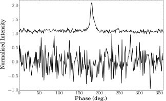
Figure 1: Average emission profiles for PSR J1634$-$5107 from the longest observations, separated by emission mode and normalised by their peak intensities. Bottom: OFF profile from an 4.5 h observation taken on 2002 September 13 at 04:52:05 UTC. Top: ON profile from a 33 min observation recorded on 2002 January 19 at 19:12:26 UTC, offset vertically for clarity. Note that the flux density of the OFF emission is $\lesssim 1.7\pm 0.5\,\%$ that of the ON emission for these data.

3.1.2 PSR J1717$-$4054

PSR J1717$-$4054 was detected in 119 out of the 371 observations analysed, and was observed to transition between its ON and OFF modes on 38 occasions. Analysis of the sub-integration data for each observation showed that the source was ON for a total of 8.6 h of the 36.7 h data set. This equates to a $\mathrm{NF}=77\pm 5\,\%$ $-$ using the error estimation method presented in $\S$ 3.1.1 $-$ which is consistent with the findings of both Johnston et al. (1995) and O’Brien et al. (2006). We also infer the average transition timescale to be $\sim$56 min from the total observation length and number of fully resolved mode transitions ($T_{\mathrm{obs}}/N_{\mathrm{switch}}$).

The null lengths in the sub-integration data were observed to span from 0.5 to $\gtrsim 64$ min. Whereas, the ON phases were observed to last between 0.5 and 12.5 min in individual observations. Given the poor constraints on the upper limits of each emission timescale, we also analysed successive contiguous observations which were not separated by more than 10 min. From this analysis, we infer a maximum ON timescale of 16.2 min and the same maximum OFF timescale of $\gtrsim 64$ min. Note that this analysis does not completely constrain the possible range of ON timescales due to inadequate observation cadence. Therefore, it is possible the maximum ON timescale could be longer than that inferred from this work. The variability of the source is demonstrated in an hour-long observation shown in Fig. 2.

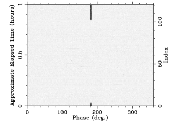
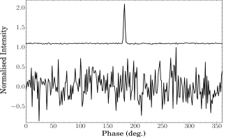
Figure 2: An hour-long observation of PSR J1717$-$4054 recorded on 2012 October 10 at a centre frequency of 3094 MHz. Top panel: Sub-integration versus phase intensity map showing the pulsar transition between the ON and OFF modes and back again. Bottom panel: Average profiles for the corresponding OFF (bottom) and ON (top) sub-integrations displayed in the top panel, normalised by their peak intensities and offset vertically for clarity. Note that no emission is detected through integration of 48 min of data. The null confusion limit is also $\lesssim 0.8\pm 0.2\,\%$ of the flux density of the ON emission for these data.

Upon inspection of the available single-pulse data, we were also able to confirm that the source transitions between emission modes over timescales of $\lesssim 1\,P$. In addition, we found that the source exhibits a bimodal distribution of nulls. That is, the source preferentially undergoes nulls over timescales of $\sim 1-40\,P$ or $\gtrsim 340\,P$. We also note that emission bursts from the pulsar only last $\sim 1-200\,P$. Therefore, it is clear that the majority of the short timescale nulls will not be resolved in the sub-integration data of the ON phases where $t_{\mathrm{sub}}\gtrsim 60$ s. Thus, the interpretation of the ON emission timescales is dependent on the observation setup.

The above results are consistent with the results of O’Brien (2010), but are markedly different from the NF estimate of Wang et al. (2007) taken from a single observation. We attribute this to variation in the OFF and ON timescales, where the wide range of activity timescales observed in our data set can lead to variation in NF estimates between observations.

3.1.3 PSR J1853$+$0505

PSR J1853$+$0505 was detected in 93 out of the 392 observations analysed, and was observed to transition between its ON and OFF states on 29 occasions in individual observing runs (see, e.g., Fig. 3). Analysis of the sub-integration data showed that the pulsar was ON for a total of 17.8 h of the 92.8 h combined data set. For the LAFB data set we further integrated observations to sub-integration times of $\gtrsim 6$ min, to counter the low bandwidth and subsequent reduction in sensitivity. Whereas, we were still able to probe typical timescales of $\gtrsim 1$ min for the Parkes and LDFB data given the greater sensitivity.

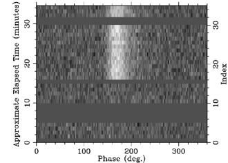
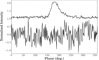
Figure 3: A 34.4 min long observation of PSR J1853$+$0505 recorded on 2001 June 17 at a centre frequency of 1374 MHz. Top panel: Sub-integration versus phase intensity map showing the pulsar transition between the OFF and ON modes. Note that the blank horizontal lines represent sub-integrations weighted to zero from the RFI excision process. Bottom panel: Average profiles for the corresponding OFF (bottom) and ON (top) sub-integrations displayed in the top panel, normalised by their peak intensities and offset vertically for clarity. Note that no emission is detected through integration of 9 min of OFF data. The null confusion limit is also $\lesssim 3\pm 1\,\%$ of the ON emission for these data.

In addition to the strong detections, we noted that the source appears extremely weak in 12 of the observations (refer to Fig. 4). This weak emission is not detected over timescales of less than several minutes. Rather, it can only be observed through integration of sufficiently long observations (i.e. $\gtrsim 10$ min), which is similar to the underlying emission observed in a number of sources (see, e.g., Esamdin et al. 2005; Wang et al. 2007; Young et al. 2014; Sobey et al. 2014).

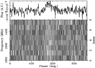
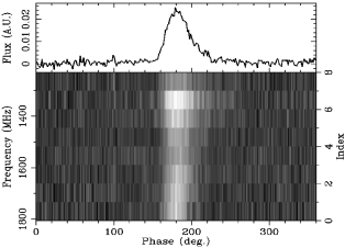
Figure 4: Two 15 min observations of PSR J1853$+$0505, obtained at 1518 MHz, demonstrating the different emission states of the source. The top plot shows a weak detection of the source, which was obtained an hour before an OFF detection and 2 hours before the strong detection, shown in the bottom plot. The integrated profile and frequency versus phase intensity plot is displayed for each observation, in the top and bottom panels of each plot, respectively.

Remarkably, weak-mode transitions were also observed in two observations, spaced over a year apart. In the first observation, the pulsar exhibited weak-emission for $\sim 16$ min, then abruptly transitioned to its strong mode (i.e. between $\sim 1$ min sub-integrations) for the remaining $\sim 19$ min of the observation. In the other observation, the source emitted in its strong mode for $\lesssim 1$ min, then abruptly switched to its weak mode for the remaining $\sim 9$ min. These attributes indicate that the weak emission mode is relatively stable, which occurs between strong and OFF phases of emission. The above also suggests a common driving mechanism for the separate emission modes, due to the consistency of their transition timescales.

Although the LAFB data was subject to more RFI, compared with data obtained with the other backends, the longer observing runs recorded provide greater constraints on the cumulative ON and OFF timescales of the source. In these data, we did not resolve any ON modes of less than 30 min in duration, nor did we observe any greater than 2 h in length. Similarly, the minimum and maximum OFF timescales were found to be 40 min and $\gtrsim 7$ h $20$ min, respectively. However, we emphasise caution in assuming the upper limit for the maximum OFF length, given that the LAFB data were limited in being able to probe weak-mode detections.

We calculated NF estimates for both the LAFB ($\mathrm{NF}_{{}_{\mathrm{LAFB}}}$ $=$ $86\,\pm 6\,\%$) and combined Parkes-LDFB ($\mathrm{NF}_{{}_{\mathrm{cmbd}}}$ $=$ $67\,\pm\,8\,\%$) data sets separately, due to the different observation sensitivities. Considering the prevalence of weak emission in the combined Parkes and LDFB data set, i.e. $\sim$11$\,\%$ of the total time, we suspect that the NF estimate for the LAFB data is most likely overestimated. As such, we assume the NF from the combined Parkes-LDFB data provides a better representation of the variability of the source. We also infer an average timescale of $\sim$3.2 h between contiguous ON modes from the total observation length and number of observed transitions.

3.2 Flux Density Limits

The detection of particularly weak emission in a number of objects $-$ through sufficient pulse integration (see, e.g., Esamdin et al. 2005; Wang et al. 2007; Young et al. 2014) or migration to lower observing frequencies (Sobey et al., 2014) $-$ raises speculation as to whether all nulls actually represent weak emission states or not. This is punctuated by the fact that every telescope has a specific flux density limit, for a given integration time, which may or may not allow the detection of such low intensity emission states. With the above in mind, we sought to place upper limits on the flux densities of the separate emission modes ($S_{\mathrm{off}}:S_{\mathrm{on}}$) for the pulsars in this study, so as to characterise the possibility of null confusion in our data.

To estimate the flux density of the sources, during their separate emission modes, we formed time- and frequency-averaged profiles for corresponding observations obtained with the Parkes telescope. Observations were aligned using the timing solution for each source, prior to integration. We then used the modified radiometer equation to estimate the average flux densities attributed to each mode from the mean signal-to-noise ratios (SNRs; see, e.g., Lorimer & Kramer 2005). Here, we assume that the dominant uncertainties arise from gain and system temperature variations with respect to elevation for a given observing session. We thus conservatively assume a $20\,\%$ variation in flux density between each observation. We note, however, that the actual uncertainites on our flux measurements are likely to be lower than this upper limit, especially for the 10/50cm observations which were obtained in close succession. Table 2 shows the result of this analysis for the three sources.

Table 2: Average pulse properties for PSRs J1634$-$5107, J1717$-$4054 and J1853$+$0505. The pulsar J2000 designation, observation frequency, bandwidth, number of observations used for each fold and total integration length are denoted by PSR J, $\nu$, $\Delta\nu$, $N_{\mathrm{on,off}}$ and $T_{\mathrm{on,off}}$, respectively. The mean signal-to-noise ratio, average equivalent width and flux density are represented by $\mathrm{SNR}$, $W_{\mathrm{eq}}$ and $S_{\mathrm{on,off}}$, respectively. The upper limit on the OFF:ON flux density is also denoted by $S_{\mathrm{off}}:S_{\mathrm{on}}$. Note that we assume an upper limit of $\mathrm{SNR}=3$ for the OFF emission. The uncertainties in the flux densities are also quoted in parentheses with respect to the least significant digit.

PSR	$\nu$	$\Delta\nu$	$N_{\mathrm{on}}$	$N_{\mathrm{off}}$	$T_{\mathrm{on}}$	$T_{\mathrm{off}}$	$\mathrm{SNR}$	$W_{\mathrm{eq}}$	$S_{\mathrm{on}}$	$S_{\mathrm{off}}$	$S_{\mathrm{off}}:S_{\mathrm{on}}$
	(MHz)	(MHz)			(s)	(s)		(ms)	(mJy)	($\mu$Jy)	($10^{-3}$)
J1634$-$5107	1374	288	26	136	10986.8	85650.4	161.0	14.4	0.40 (8)	$\lesssim 2.6$ (5)	$\lesssim 7$ (2)
	1518	576	13	27	7488.0	17072.6	119.4	15.7	0.22 (4)	$\lesssim 3.6$ (8)	$\lesssim 17$ (5)
J1717$-$4054	732	64	2	2	874.9	3784.9	132.5	69.6	7 (1)	$\lesssim 80$ (20)	$\lesssim 11$ (3)
	1374	288	44	55	12152.8	16104.4	1393.8	13.3	2.3 (5)	$\lesssim 4.4$ (9)	$\lesssim 1.9$ (6)
	1518	576	8	7	2156.5	2096.6	406.5	11.6	0.9 (2)	$\lesssim 7$ (1)	$\lesssim 7$ (2)
	3094	1024	2	2	874.9	3963.3	158.2	7.8	0.6 (1)	$\lesssim 5$ (1)	$\lesssim 9$ (3)
J1853$+$0505	1374	288	27	11	16466.9	3768.0	305.8	105.7	1.3 (3)	$\lesssim 27$ (5)	$\lesssim 20$ (6)
	1518	576	10	1	8985.6	898.6	190.9	93.2	0.6 (1)	$\lesssim 30$ (6)	$\lesssim 50$ (20)

Both PSRs J1634$-$5107 and J1853$+$0505 were not observed during their ON modes while the 10/50cm receiver was in use. Therefore, we cannot provide any constraints on the ON or OFF average flux densities in either the 10- or 50-cm band for these sources.

Comparing the flux densities of PSRs J1634$-$5107, J1717$-$4054 and J1853$+$0505, we place upper limits on their $S_{\mathrm{off}}:S_{\mathrm{on}}$ values of $\lesssim(7\pm 2)\times 10^{-3}$, $\lesssim(1.9\pm 0.6)\times 10^{-3}$ and $\lesssim(2\pm 0.6)\times 10^{-3}$, respectively. The stringent null confusion limit placed on PSR J1717$-$4054 indicates that the source could undergo deep nulls which are well below the sensitivity threshold of the Parkes observing system. Whereas, the limits placed on PSR J1634$-$5107 and particularly PSR J1853$+$0505 indicates that null confusion could occur in these sources. For PSR J1853$+$0505, this is consistent with its observed weak emission, which is detected just above the noise level (see also $\S$ 6.2).

4 Timing

Considering the $\dot{\nu}$ variations observed in several moding and/or nulling objects (Lyne et al., 2010), we sought to characterise and compare the timing properties of the pulsars in our study. Here, we computed the best-fit timing solutions for the objects using the TEMPO2 package and the PSRCHIVE software suite.

Due to the low number of 10/50cm ON observations, we only considered observations obtained at L-band for this analysis. Here, we formed analytic templates from the highest-SNR PAFB (all sources), PDFB (PSRs J1634$-$5107 and J1717$-$4054), LDFB (PSR J1853$+$0505) and LAFB (PSR J1853$+$0505) profiles using paas. Pulse time-of-arrivals (TOAs; e.g. Manchester & Taylor 1977) were generated through cross-correlation between the templates and corresponding observations for each source using pat. Note that instrumental delays between receivers and/or backends were also fitted in tempo2. This process also ensures that delays caused by inaccurate alignment of the different templates used for the same source were accounted for. The results of this analysis are presented in Table 3 and Fig. 5.

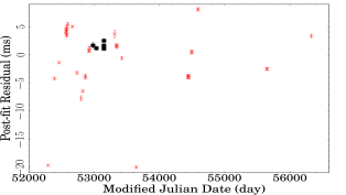
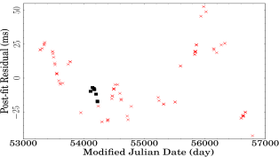
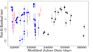
Figure 5: Top panel: best-fit timing residuals for PSR J1634$-$5107, from an 11.1-yr span of observations, with crosses and squares denoting TOAs obtained at $\sim$1374 MHz and 1518 MHz, using the Multibeam and H-OH receivers, respectively. Centre panel: best-fit timing residuals for PSR J1717$-$4054, from 9.6 yr of data, with crosses and squares denoting TOAs obtained at 1374 MHz and 1518 MHz, using the Multibeam and H-OH receivers, respectively. Bottom panel: best-fit timing residuals for PSR J1853$+$0505, from an 11.9-yr long data set, with circles, crosses and squares denoting TOAs obtained with the PAFB (1374 MHz and 1518 MHz), LAFB (1396 MHz) and LDFB (1402 MHz and 1520 MHz) backends, respectively.

Table 3: Fitted and derived properties of PSRs J1634$-$5107, J1717$-$4054 and J1853$+$0505 from their best-fit timing solutions. The distance of each source is taken from the NE2001 model, and is assumed to have a $20\,\%$ uncertainty. Errors are displayed in the parentheses, for parameters which were fitted, and are in units of the least-significant digit.

PSR	RA (J2000)	Dec. (J2000)	$\nu$	$\dot{\nu}$	DM	d	Epoch	$N_{\mathrm{TOA}}$	$T_{\mathrm{s}}$	RMS
	( h : m : s )	( ∘ : ′ : ′′ )	(s-1)	($10^{-15}$ s-2)	(pc cm-3)	(kpc)	(MJD)		(yr)	($\mu$s)
J1634$-$5107	16:34:04.99(8)	$-$51:07:45.6(9)	1.97100259922(5)	$-$6.1167(5)	373(2)a	6.1	54420	50	11.1	4537
J1717$-$4054	17:17:51.8(1)	$-$41:03:20(5)	1.12648304468(3)	$-$4.6737(7)	306.9(1)b	4.7	55035	108	9.6	22011
J1853$+$0505	18:53:04.32(4)	$+$05:05:29(1)	1.10480469655(3)	$-$1.5631(2)	279(3)c	6.6	53982	89	11.9	7857

^aLorimer et al. (2006), ^bKerr et al. (2014), ^cHobbs et al. (2004).

We find that the timing solutions for PSRs J1634$-$5107 and J1853$+$0505 are consistent with previous findings (Hobbs et al., 2004; Lorimer et al., 2006). In contrast to PSR J1853$+$0505, we note that the residuals of PSR J1634$-$5107 are not white, indicating that $\dot{\nu}$ variations may exist in this source. However, our observing cadence is unsufficient here to infer anything conclusive about spin-down variations in the object. We also find substantial timing noise in PSR J1717$-$4054 ($\mathrm{RMS}\sim 22$ ms; c.f. Hobbs et al. 2004), which is comparable to that observed in a large number of sources (Hobbs et al., 2010).

The timing noise in PSR J1717$-$4054 can be interpreted as systematic $\dot{\nu}$ variations. To quantify this, we performed stride fits across its timing data using tempo2, following the method outlined in Lyne et al. (2010). Here, we used data windows of 200 d in length, and stride steps of 50 d, to provide the necessary timing accuracy while not compromising too heavily on time resolution. From this analysis, we find that the source exhibits a peak-to-peak spin-down variation $\Delta\nu_{\mathrm{pk}}=1.53\pm 0.03\times 10^{-15}$ s^-2 and a fractional spin-down variation $|\Delta\nu_{\mathrm{pk}}|/\langle\dot{\nu}\rangle=33\pm 1\,\%$ over the course of hundreds of days (see Fig. 6).

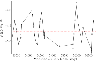
Figure 6: Variation in $\dot{\nu}$ against time for PSR J1717$-$4054, using fit windows of 200 d and stride steps of 50 d. The measured $\langle\dot{\nu}\rangle$ from the overall timing solution is also overlaid.

Following the method outlined in Young et al. (2012), we performed WWZ analysis on the $\dot{\nu}$ data to determine if the variations were periodic. However, we find that the cadence of our data is too poor to allow any periodic trend to be accurately determined. We were also unable to detect any significant pulse shape variation over time due to the narrow pulse longitude range over which emission is detected. This precludes any direct correlation between $\dot{\nu}$ variation and pulse shape variation over time.

5 Polarimetric Properties

We also analysed polarimetric Multibeam observations of PSRs J1634$-$5107 and J1717$-$4054. As no single pulse observations were available in these data, we present only the average pulse polarisation properties. The polarisation calibration was carried out following the scheme outlined in Weltevrede & Johnston (2008).

5.1 PSR J1634$-$5107

We used 12 Multibeam observations to probe the polarimetric properties of PSR J1634$-$5107. These were aligned, using the timing solution presented in Table 3, and then averaged to produce an integrated profile from the 42 min of data using the PSRCHIVE software suite. We determined the rotation measure (RM; see, e.g., Lorimer & Kramer 2005) of the source, $\mathrm{RM}=-151\pm 8$ rad m^-2, for the first time using the rmfit package (Noutsos et al., 2008).

After correcting for RM, we analysed the intrinsic Stokes parameters ($I$,$Q$,$U$,$V$) and degree of linear ($L/I=\sqrt{Q^{2}+U^{2}}/I$) and circular ($V/I$) polarisation for the source (see top panel of Fig. 7). Using a $3\sigma$ limit for the polarisation data, we found that the pulsar exhibits high linear ($\langle L/I\rangle=19\pm 2\,\%$) and modest circular ($\langle|V|/I\rangle=10\pm 1\,\%$) polarisation, when averaged over bins within the $10\,\%$ intensity pulse width ($W_{10}$) range. We also computed the maxima of the polarisation profiles; i.e. $(L/I)_{\mathrm{max}}=40\pm 10\,\%$ and $(|V|/I)_{\mathrm{max}}=30\pm 20\,\%$. Here, we quote uncertainties on the degrees of linear and circular polarisation in terms of their respective quadrature errors; e.g. $\Delta L=\sigma_{\mathrm{L}}\sqrt{N_{\mathrm{on}}}$, where $\sigma_{\mathrm{L}}$ is the RMS of $L$ in the off-pulse region and $N_{\mathrm{on}}$ is the number of on-pulse bins considered).

Further to the above, we sought to determine the magnetic inclination angle of the source ($\alpha$) and the impact parameter of the LOS ($\beta$). For this analysis, we fitted the polarisation position angles (PAs) of the integrated emission with the rotating vector model (RVM; Radhakrishnan & Cooke 1969), adopting the $\chi^{2}$ minimisation technique presented by Rookyard et al. (2015) to obtain fit constraints with $3\sigma$ PA values.

We find that the best-fit to our data is consistent with the RVM (see Fig. 7). However, we cannot place rigorous constraints on the $\alpha$ and $\beta$ parameters due to the low number of significant PA data points available. Instead, if we assume $\alpha=$$$, we can estimate the maximum $\beta$ value ($\beta_{90}$) from the maximum gradient $(d\Psi$/$d\phi)_{\mathrm{max}}$ of the RVM fit (Komesaroff 1970; see below). In the general case, $\beta$ is less than this value:

$$\beta_{90}=\mathrm{sin}^{-1}\left[\mathrm{sin}\,($$)\,\left(\frac{d\Psi}{d\phi}\right)^{-1}_{\mathrm{max}}\right]\sim$$\,.$$ (1)

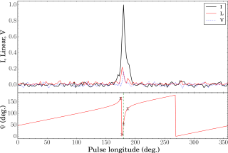
Figure 7: The best RVM fit to the integrated 42 min observation of PSR J1634$-$5107. Top panel: the average emission properties of the integrated observation, showing the total intensity profile, as well as the linear and circular polarisation profiles. Bottom panel: integrated PA data (crosses), with the best-fitting RVM (solid line) and location of the PA swing inflection point ($\phi_{0}$; dotted line) overlaid.

5.2 PSR J1717$-$4054

We used 35 Multibeam observations to characterise the polarimetric properties of PSR J1717$-$4054. The 146 min of data were aligned and folded, using the same method as in $\S$ 5.1, to produce an integrated profile for this analysis. We again used rmfit to measure an $\mathrm{RM}=-809\pm 3$ rad m^-2 for the source. This best-fit RM value, which represents a refinement of the result of Kerr et al. (2014), was then used to correct the average profile, resulting in the profile shown in the top panel of Fig. 8.

We find that the source exhibits modest linear ($\langle L/I\rangle=8.1\pm 0.1\,\%$) and circular polarisation ($\langle|V|/I\rangle=4.9\pm 0.1\,\%$), when averaged over the $W_{10}$ range (with $(L/I)_{\mathrm{max}}=30\pm 4\,\%$ and $(V/I)_{\mathrm{max}}=6.9\pm 0.2\,\%$). We also attempted to fit the PA data for the source, using the same method as in $\S$ 5.1, but could not obtain any constraints on the values of $\alpha$ or $\beta$ from the resultant reduced $\chi^{2}$ surface. This is due to the clustering of the PA data points which are not highly constrained by the RVM (see bottom panel Fig. 8).

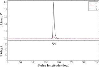
Figure 8: The average emission properties of the 146 min observation of PSR J1717$-$4054. Top panel: the total intensity (black line), linear (red line) and circular (blue line) polarisation profiles. Bottom panel: integrated PA data for the average profile.

6 Discussion and Conclusions

6.1 Emission Variability

Thorough analysis of our extensive data set has shown that PSRs J1634$-$5107, J1717$-$4054 and J1853$+$0505 exhibit long term nulls and emission phases (i.e. minutes to many hours), as well as substantial NFs (i.e. $\sim 67\,\%-90\,\%$). Remarkably, PSR J1853$+$0505 was also shown to exhibit a weak emission state, in addition to its strong and null states (see $\S$ 6.2).

Short timescale nulling ($\sim 1-40~{}P$) was discovered in PSR J1717$-$4054, during its ON phases, which acts to modulate the NF and average detection rate of the source over sub-integration timescales. This behaviour was also discovered in an independent analysis performed by Kerr et al. (2014), who analysed the same archival data and two dedicated 9.5-h single-pulse observations. The latter observing runs constrained a number of mode transitions and thus allowed tentative limits to be placed on the average ON and OFF emission timescales of $t_{\mathrm{{on}}}=1200\pm 700$ s and $t_{\mathrm{{on}}}=7000\pm 5000$ s, respectively. These average emission durations are found to be consistent with the results obtained in this work, and indicate that the source exhibits a wide range of emission timescales. Thus accounting for varied NF reports in the literature.

Overall, the above results place PSRs J1634$-$5107, J1717$-$4054 and J1853$+$0505 at the extreme end of the ‘nulling continuum’, where there is a current deficit of known objects (see, e.g., Keane et al. 2011; Burke-Spolaor et al. 2011). For such sources, it is clear that long observations ($\gtrsim 1$ h) are required to best characterise their emission properties, as demonstrated in Kerr et al. (2014).

6.2 Deep Nulls or Weaker Emission States?

PSR J1853$+$0505 is shown to exhibit three emission states: a weak, strong and null state. During the weak mode, emission is barely detected above the noise level in our observations. This behaviour is remarkably similar to that observed in PSR J1107$-$5907, where emission at the lowest end of its weak-mode pulse-energy distribution is easily confused with nulls (Young et al., 2014). Similar to PSR J1107$-$5907, integration of $\gtrsim 10^{3}$ pulses is required to detect the particularly weak emission of PSR J1853$+$0505, leading to an average $S_{\mathrm{off}}:S_{\mathrm{weak}}\lesssim 0.11\pm 0.03$ at 1374 MHz. These similarities indicate a close connection between the two objects which, in turn, advocates further, more detailed analysis of the different emission modes of PSR J1853$+$0505.

For the other sources in our study, PSRs J1634$-$5107 and J1717$-$4054, only two discrete modes were observed in each object. From this work, we place null confusion limits of $\lesssim(7\pm 2)\times 10^{-3}$ and $\lesssim(1.9\pm 0.6)\times 10^{-3}$ on these pulsars, respectively. Considering the fact that PSR J1634$-$5107 is approximately 3 times fainter than PSR J1853$+$0505, it is unsurprising that observations of the former did not result in the discovery of a weaker emission state. As such, PSR J1634$-$5107 could exhibit a particularly weak emission state which is not probed by our observations, or it could actually undergo deep nulls. In the case of PSR J1717$-$4054, we suspect that the source exhibits the latter. This is supported by independent analysis performed by Kerr et al. (2014), which resulted in a more stringent limit on its null confusion limit (i.e. $\lesssim 10^{-3}$). Thus, our observations clearly do not probe a potential lower intensity emission state in this object.

Since particularly weak emission has been reported in this work, and in a number of other pulsars (e.g. $S_{\mathrm{weak}}:S_{\mathrm{strong}}\lesssim 2\times 10^{-3}$ for J1107$-$1107; Young et al. 2014), it is possible that pulse nulling may only represent an instrumental sensitivity bias on certain members of the pulsar population. Overall, these findings provide additional motivation to perform more regular and longer observations of nulling objects, which will likely only be possible with next generation telescopes such as MeerKAT and the SKA. Such steps would ultimately help to construct a census of nulls and mode transitions in the pulsar population, which is required to help form a fully consistent pulsar emission model.

6.3 Timing Properties

We have confirmed and updated the timing solutions of PSRs J1634$-$5107, J1717$-$4054 and J1853$+$0505, using the longer data spans available in this work. Both PSRs J1634$-$5107 and J1853$+$0505 are found to exhibit weak timing noise, in spite of their extreme variability. Whereas, PSR J1717$-$4054 is shown to exhibit modest timing noise, similar to that observed in a number of pulsars which switch between magnetospheric states (Hobbs et al., 2010; Lyne et al., 2010).

Upon further investigation of the timing behaviour of PSR J1717$-$4054, we found that its timing noise can be accounted for by substantial variation in $\dot{\nu}$ over hundreds of days (c.f. Lyne et al. 2010). This variation is too slow to be associated with transitions between ON and OFF phases in its emission. Therefore, it is likely that the source also exhibits emission variability over similarly long timescales. While we were unable to confirm this hypothesis through analysis of our data, we predict that more frequent detections of this source with high-time resolution data will lead to a direct association with $\dot{\nu}$ variation. Overall, it is clear that PSR J1717$-$4054 is a multi-state switching object, which can be used to probe both short- and long-timescale variations in pulsar magnetospheres.

6.4 Polarimetric Findings

We have presented the first measurement of the RM for PSR J1634$-$5107, which has enabled us to fit its $\alpha$ and $\beta$ parameters. While we were unable to place constraints on $\alpha$, we were able to infer $\beta_{90}\sim$$$. Under the assumption that radio beams are comprised of core and conal emission components, we can determine $\alpha$ from the observed pulse width of the core ($W^{\mathrm{core}}_{50}$; Rankin 1990):

$$\alpha=\mathrm{sin}^{-1}\left(\frac{$$}{W^{\mathrm{core}}_{50}\,P^{\,0.5}}\right)\,.$$ (2)

The emission profile of J1634$-$5107, can be described by a strong core component, flanked by two conal emission components (see Fig. 7). We thus estimate $W^{\mathrm{core}}_{50}=$$$ and $\alpha\sim$$$. However, we stress that longer polarimetric observations of the source in its ON state, with higher time resolution, are required to better constrain its emission geometry and verify our results.

We also estimate an $\mathrm{RM}=-809\pm 3$ rad m^-2 for PSR J1717$-$4054. This value is consistent with the result of Kerr et al. (2014) and is found to be one of the highest values measured for a pulsar not located in a globular cluster (see, e.g., Noutsos et al. 2008 and references therein). After correcting the source’s integrated profile for RM, we also tried to fit the RVM to its PA data. However, we were unable to obtain any constraints on $\alpha$ or $\beta$ due to the clustering of PA data points across the narrow pulse profile, which is again consistent with the result of Kerr et al. (2014). Nevertheless, further investigation into the polarimetric properties of the source would be interesting to shed light on its short-timescale variability.

7 Acknowledgements

We would like to thank M. Serylak and the anonymous referee for useful comments which have improved this manuscript. NJY also acknowledges financial support from the South African SKA (SKA SA) project.

References

- Backer (1970) Backer D. C., 1970, 228, 1297
- Bhat et al. (2004) Bhat N. D. R., Cordes J. M., Camilo F., Nice D. J., Lorimer D. R., 2004, ApJ, 605, 759
- Brook et al. (2014) Brook P. R., Karastergiou A., Buchner S., Roberts S. J., Keith M. J., Johnston S., Shannon R. M., 2014, ApJL, 780, L31
- Burke-Spolaor et al. (2011) Burke-Spolaor S., Bailes M., Johnston S., Bates S. D., Bhat N. D. R., Burgay M., D’Amico N., Jameson A., Keith M. J., Kramer M., et al. 2011, MNRAS, 416, 2465
- Camilo et al. (2012) Camilo F., Ransom S. M., Chatterjee S., Johnston S., Demorest P., 2012, ApJ, 746, 63
- Cordes & Lazio (2002) Cordes J. M., Lazio T. J. W., 2002, preprint (arXiv:astro-ph/0207156)
- Cordes & Shannon (2008) Cordes J. M., Shannon R. M., 2008, ApJ, 682, 1152
- Deshpande & Rankin (2001) Deshpande A. A., Rankin J. M., 2001, MNRAS, 322, 438
- Dyks et al. (2005) Dyks J., Zhang B., Gil J., 2005, ApJ, 626, L45
- Esamdin et al. (2005) Esamdin A., Lyne A. G., Graham-Smith F., Kramer M., Manchester R. N., Wu X., 2005, MNRAS, 356, 59
- Gajjar et al. (2012) Gajjar V., Joshi B. C., Kramer M., 2012, MNRAS, 424, 1197
- Hankins et al. (2003) Hankins T. H., Kern J. S., Weatherall J. C., Eilek J. A., 2003, Nature, 422, 141
- Hermsen et al. (2013) Hermsen W., Hessels J. W. T., Kuiper L., van Leeuwen J., Mitra D., de Plaa J., Rankin J. M., Stappers B. W., Wright G. A. E., Basu R., et al. 2013, 339, 436
- Hobbs et al. (2004) Hobbs G., Faulkner A., Stairs I. H., Camilo F., Manchester R. N., Lyne A. G., Kramer M., D’Amico N., Kaspi V. M., Possenti A., McLaughlin M. A., Lorimer D. R., Burgay M., Joshi B. C., Crawford F., 2004, MNRAS, 352, 1439
- Hobbs et al. (2010) Hobbs G., Lyne A. G., Kramer M., 2010, MNRAS, 402, 1027
- Hobbs et al. (2004) Hobbs G., Lyne A. G., Kramer M., Martin C. E., Jordan C., 2004, MNRAS, 353, 1311
- Hobbs et al. (2011) Hobbs G., Miller D., Manchester R. N., Dempsey J., Chapman J. M., Khoo J., Applegate J., Bailes M., Bhat N. D. R., Bridle R., et al. 2011, PASA, 28, 202
- Hobbs et al. (2006) Hobbs G. B., Edwards R. T., Manchester R. N., 2006, MNRAS, 369, 655
- Hotan et al. (2004) Hotan A. W., van Straten W., Manchester R. N., 2004, PASA, 21, 302
- Janssen & van Leeuwen (2004) Janssen G. H., van Leeuwen J., 2004, 425, 255
- Johnston et al. (1992) Johnston S., Lyne A. G., Manchester R. N., Kniffen D. A., D’Amico N., Lim J., Ashworth M., 1992, MNRAS, 255, 401
- Johnston et al. (1995) Johnston S., Manchester R. N., Lyne A. G., Kaspi V. M., D’Amico N., 1995, A&A, 293, 795
- Jones (2011) Jones P. B., 2011, MNRAS, 414, 759
- Keane (2013) Keane E. F., 2013, in van Leeuwen J., ed., IAU Symposium Vol. 291 of IAU Symposium, Radio pulsar variability. pp 295–300
- Keane et al. (2011) Keane E. F., Kramer M., Lyne A. G., Stappers B. W., McLaughlin M. A., 2011, MNRAS, 415, 3065
- Keith et al. (2013) Keith M. J., Shannon R. M., Johnston S., 2013, MNRAS, 432, 3080
- Kerr et al. (2014) Kerr M., Hobbs G., Shannon R. M., Kiczynski M., Hollow R., Johnston S., 2014, MNRAS, 445, 320
- Knispel et al. (2013) Knispel B., Eatough R. P., Kim H., Keane E. F., Allen B., Anderson D., Aulbert C., Bock O., Crawford F., Eggenstein H.-B., et al. 2013, ApJ, 774, 93
- Komesaroff (1970) Komesaroff M. M., 1970, 225, 612
- Kramer et al. (2006) Kramer M., Lyne A. G., O’Brien J. T., Jordan C. A., Lorimer D. R., 2006, 312, 549
- Li et al. (2012) Li J., Spitkovsky A., Tchekhovskoy A., 2012, ApJL, 746, L24
- Lorimer et al. (2006) Lorimer D. R., Faulkner A. J., Lyne A. G., et al. 2006, MNRAS, 372, 777
- Lorimer & Kramer (2005) Lorimer D. R., Kramer M., 2005, Handbook of Pulsar Astronomy. Cambridge University Press, Cambridge
- Lorimer et al. (2012) Lorimer D. R., Lyne A. G., McLaughlin M. A., Kramer M., Pavlov G. G., Chang C., 2012, ApJ, 758, 141
- Lyne et al. (2013) Lyne A., Graham-Smith F., Weltevrede P., Jordan C., Stappers B., Bassa C., Kramer M., 2013, Science, 342, 598
- Lyne et al. (2010) Lyne A., Hobbs G., Kramer M., Stairs I., Stappers B., 2010, 329, 408
- Manchester et al. (2013) Manchester R. N., Hobbs G., Bailes M., et al. 2013, PASA, 30, 17
- Manchester & Taylor (1977) Manchester R. N., Taylor J. H., 1977, Pulsars. Freeman, San Francisco
- McLaughlin et al. (2006) McLaughlin M. A., Lyne A. G., Lorimer D. R., Kramer M., Faulkner A. J., Manchester R. N., Cordes J. M., Camilo F., Possenti A., Stairs I. H., et al. 2006, 439, 817
- Melikidze & Gil (2006) Melikidze G., Gil J., 2006, Chinese Journal of Astronomy and Astrophysics Supplement, 6, 020000
- Noutsos et al. (2008) Noutsos A., Johnston S., Kramer M., Karastergiou A., 2008, MNRAS, 386, 1881
- O’Brien (2010) O’Brien J., 2010, PhD thesis, The University of Manchester
- O’Brien et al. (2006) O’Brien J. T., Kramer M., Lyne A. G., Lorimer D. R., Jordan C. A., 2006, Chinese J. Astron. Astrophys. Suppl., 6, 020000
- Radhakrishnan & Cooke (1969) Radhakrishnan V., Cooke D. J., 1969, Astrophys. Lett., 3, 225
- Rankin (1990) Rankin J. M., 1990, ApJ, 352, 247
- Rankin & Wright (2007) Rankin J. M., Wright G. A. E., 2007, MNRAS, 379, 507
- Rookyard et al. (2015) Rookyard S. C., Weltevrede P., Johnston S., 2015, MNRAS, 446, 3367
- Rosen et al. (2011) Rosen R., McLaughlin M. A., Thompson S. E., 2011, ApJL, 728, L19
- Sobey et al. (2014) Sobey C., Young N. J., Hessels J. W. T., et al. 2014, MNRAS, submitted
- Timokhin (2010) Timokhin A. N., 2010, MNRAS, 408, L41
- Wang et al. (2007) Wang N., Manchester R. N., Johnston S., 2007, MNRAS, 377, 1383
- Weltevrede & Johnston (2008) Weltevrede P., Johnston S., 2008, MNRAS, 387, 1755
- Young et al. (2013) Young N. J., Stappers B. W., Lyne A. G., Weltevrede P., Kramer M., Cognard I., 2013, MNRAS, 429, 2569
- Young et al. (2012) Young N. J., Stappers B. W., Weltevrede P., Lyne A. G., Kramer M., 2012, MNRAS, 427, 114
- Young et al. (2014) Young N. J., Weltevrede P., Stappers B. W., Lyne A. G., Kramer M., 2014, MNRAS, 442, 2519
- Zhang et al. (2007) Zhang B., Gil J., Dyks J., 2007, MNRAS, 374, 1103