South Pointing Chariot: An Invitation to Differential Geometry

Abstract

We introduce the south-pointing chariot, an intriguing mechanical device from ancient China. We use its ability to keep track of a global direction as it travels on an arbitrary path as a tool to explore the geometry of curved surfaces. This takes us as far as a famous result of Gauss on the impossibility of a faithful map of the globe, which started off the field of differential geometry. The reader should get a view into how geometers think and an introduction to important early results in the field, but should need no more than a solid background in calculus (ideally through multivariable calculus). This is achieved by relying on the reader’s visual intuition.

1 Some History, and Some Engineering

Legend tells of Huangdi, the Yellow Emperor, tamer of beasts real and supernatural, father of the Huaxia people who formed what would become China. Also inventor of the bow sling, the Chinese calendar, early astronomy, a zither, a Chinese version of football, and depending on whom you ask early Chinese writing and the growing of cereal. Four thousand years ago with the aid of his many tamed beasts he fought a famous battle with his arch-nemesis, the bronze-headed Chi-You and his $81$ horned and four-eyed brothers. Chi You confounded the Yellow Emperor by breathing out a thick fog, but the Emperor invented, apparently on the spur of the moment, an ingenious “south pointing chariot” with a figure on the top connected to the wheels in such a fashion that it always pointed south. This contraption led his army out of the fog and to victory.

It may not suprise you that modern scholars do not give complete credence to the details of this story. Among other things it is doubtful that the technology to build such a chariot could have been achieved so early. This skepticism was shared even by some early Chinese figures, such as Permanent Counsellor Gaotang Long and General Qin Lang during the Three Kingdoms period in the third century CE. Their contemporary, the engineer Ma Jun, replied to their doubt cuttingly with “Empty arguments with words cannot (in any way) compare with a test which will show practical results” and silenced them by inventing and building a version of Huangdi’s chariot. No designs or physical evidence remains, but scholars do generally credit that he built such a thing. That’s no tamed dragon, but still quite remarkable. It seems to require gearing unknown until 1720 CE. The south pointing chariot was lost and reinvented several times in Chinese history, and while there are reports of its use in military and navigation applications, all we know it was used for is ceremonial processions [NL65].

2 How it Works

If you search on a term such as “south pointing chariot” you will find videos of recreations that will illustrate how the gears allow this magic to happen. We’ll try here with words and a few pictures. First the differential.

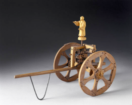
Figure 1: South pointing chariot, and the differential that makes it work

Looking at the diagram in Figure 1, we see that if the left and right axle are turning at the equal and opposite speed, the ring gear and the central axle will not turn at all. Believe me that the rate of the central axle depends linearly on the rates of the left and right axles, and you must believe that it turns at a rate proportional to the average of the rates of the left and right axles.

While driving, when you turn right your left wheel travels further than your right wheel. Your car’s differential allows the vehicle to distribute the rotation of the drive train to the two wheels as the requirements of the road demand. But Ma Jun was even cleverer with his supposed differential, because his chariot not only turned corners, but each time it did the figure on top (traditionally a statue of an authoritative gentleman pointing south) turned by exactly the same amount relative to the chariot in the opposite direction, so that (from a fixed perspective) it remained pointing in the same direction. Look a little more carefully at what happens when a vehicle turns a corner.

If as in the left side of Figure 2 the chariot has two wheels a distance $w$ apart and it rotates right on the arc of a circle of radius $r$ for an angle $\theta$ (in radians!) the left wheel travels a distance $w\theta$ more than the right wheel. If the vehicle is not traveling in an arc of a circle but along some arbitrary smooth path then trust your intuition that the path can be approximated as closely as you like by a sequence of straight lines and arcs of circles as in the right side of Figure 2. The left wheel travels $w\theta$ more than the right wheel on each arc segment, so adding these up with signs, whatever path your vehicle travels, if its total rotation is $\theta$ radians clockwise and its width is $w$ the left wheel will travel a total of $w\theta$ more than the right wheel.

Figure 2: Relating the relative distance each wheeel travels to total rotation

Returning to our friend Ma Jun, attach the left axle of the differential to the left wheel by an odd number of gears, the right axle to the right wheel by an even number of gears, and finally connect the central axle to the gentlemanly statue. If the left wheel travels with velocity $v_{l},$ its axle rotates at a rate proportional to $v_{l}.$ Each gear reverses the direction of rotation, so the left axle of the differential rotates at a rate $d\theta_{l}/dt$ proportional to $-v_{l}.$ Likewise the right axle rotates at a rate $d\theta_{r}/dt$ proportional to $v_{r}.$ That means that the statue rotates at a rate $d\theta_{s}/dt$ proportional to the average, which is to say proportional to $v_{r}-v_{l}.$ Integrating over time the statue rotates an angle $\theta_{s}$ proportional to $d_{r}-d_{l},$ the difference in the distances the two wheels travel over the course of the journey. adjust the sizes of the various gears to make that constant of proportionality $1/w,$ so that the statute rotates an angle

$$\theta_{s}=\frac{d_{r}-d_{l}}{w}=-\theta,$$

the negative of the angle the chariot rotated. That is to say, the statue points in a constant direction.

This is such a beautiful fact that as mathematics it deserves to be expressed in very precise and abstract language so as to wring every bit of meaning from it. Imagine an axis that cuts horizontally across the chariot, centered at its center, so that the left and right wheel are placed at the points $x=-w/2$ and $x=w/2$ respectively. Choose some path that you would like the chariot to travel, and let $d(x)$ be the distance a wheel placed at position $x$ would travel during this journey. So for instance $d(-w/2)=d_{l}$ and $d(w/2)=d_{r},$ as in Figure 3. Now recognize the formula for the net angle of rotation of our statue, $\!\left[d(w/2)-d(-w/2)\right]/w,$ as a difference quotient. The angle rotated, which is the negative of the angle rotated by the chariot itself, is independent of $w,$ so it is very natural to anyone who has taken calculus to observe

$$\theta_{s}=\lim_{w\to 0}\frac{d(w/2)-d(-w/2)}{w}=\frac{\delta d}{\delta w},$$

That is the angle the statue rotates is the derivative of the distance traveled by a wheel with respect to its position on the chariot. I used $\delta$ for my derivative notation principally to avoid the notational mostrosity $\frac{dd}{dx},$ but also as a sly reference to functional differentiation and the calculus of variations, which are hiding in the wings of this calculation and for which I hope to whet your appetite [Wei74, FO]. To put it a different way (and to switch to the rotation of the vehicle) the clockwise angle a vehicle rotates as it traverses a path is the rate at which the length of the path increases as you move it to the left.

Figure 3: Rotation determines how moving the path slightly to the left changes the length

3 Why It Doesn’t Work

If the wheels and gears of the device are perfectly sized and suffer from no slippage and the surface on which it travels is perfectly flat, then a south pointing chariot which starts out pointing south will always point south no matter what path it travels. Slippage and errors in sizing are not the concern of (theoretical) mathematicians, but nonflat surfaces definitely are, and here is where the chariot transforms from a historical and engineering curiosity to mathematical tool.

Imagine the chariot travels in a straight line (from a birds-eye view) over a hill, keeping the peak of the hill to its left (see Figure 4). Notice that the left wheel goes a little further uphill and a little further downhill than the right wheel. So the left wheel travels slightly further than the right, and the statue rotates slightly counterclockwise. The bird flying overhead would assert that the chariot traveled in a straight line, but a rider on the chariot, watching the statue turn, would think that the chariot had turned slightly to the right. Perhaps you share the bird’s point of view (understandably) but suspend your preconceptions and judge the two points of view objectively. In a disagreement about what constitutes a straight line, what might we take as a definition to adjudicate? Euclid famously said “a straight line is the shortest distance between two points,” raising the question: Is the bird-straight line the shortest distance between two points?

Were it the shortest distance between two points, moving it a bit to the left or right could not shorten it. But SPC, the south pointing chariot, measures the rate at which the length increases when moving the path to the left. Since the statue rotated counterclockwise, the path lengthens as it moves left and shortens as it moves right. If moving the bird-straight line to the right shortens it, it is not the shortest distance!

Well, hold on. You might reasonably argue that we are looking for the shortest distance between two fixed points and moving the path to the right, shortens the distance, but also changes the endpoints. But that is really only a technical issue. Consider a point $\epsilon$ to the right of the midpoint of SPCs path. Imagine SPC starting at the same starting point, but traveling in a bird-straight path to this slightly moved point, then a bird-straight path to its ending point. On the one hand the path has moved to the right so it is shorter, but on the other it is traversing two sides of the triangle rather than the straight path between them, so it longer. Which wins? A little unfastidious thinking should convince you that the shortening is linear in $\epsilon$ (the factor is in fact $\theta$) while the increasing is quadratic in $\epsilon$ (by Pythagoras). So if $\epsilon$ is small enough the shortening wins: Moving the path a little to the right reduces is length.

(A) SPC travels over a hill	(B) The pointer rotates counterclockwise
(C) A slightly shorter path	(D) The shortest path has no rotation

Figure 4: Traversing a Hill

If SPC travels along this new path, it rotates a little less than it did on the original path, but if the change is small enough it will still rotate. so moving it further to the right shortens it even more. Keep doing that until the statue does not rotate at all. At that point the rotation $\delta d/\delta x=0,$ which is to say that moving neither left nor right shortens the path. If there is no way to move a path slightly while keeping the endpoints fixed and make the length shorter, then the path is, at least locally, the shortest distance between those two points. In other words a line which is straight according to the birds is not straight in the sense of Euclid. But straight according to the chariot is Euclid straight. Euclid gives the nod to the chariot!

Geometers refer to a path which SPC can travel along with no rotation of the statue by the lovely term “geodesic.” So a path which is the shortest distance between two points is always a geodesic (spoiler alert: not all geodesics are the shortest distance).

A couple of details have been swept under the rug. First, recall that $\delta d/\delta x$ equals the small $w$ limit of the difference quotient $\!\left[d(w/2)-d(-w/2)\right]/w,$ and on a flat plane the difference quotient is constant and therefore equals the limit. This constancy fails on a curved surface – for instance imagine SPC that is so wide that its wheels straddle the hill and miss it entirely. So from here on assume that SPC is “sufficiently small,” that is so small compared to the topography it is exploring that the difference quotient is extremely close to its limit. Second, for the sake of simplicity I have spoken only of the total net rotation that SPC undergoes along a path. If, during some of the trip, the statue rotates clockwise while during other parts it rotates counterclockwise, to find the minimum would require perturbing to the left when it rotates clockwise and to the right when it rotates counterclockwise. This process would converge on a path where the statue does not rotate at all, not just one where the final net rotation is zero.

One final aside. Following the direction of negative derivative to a minimum where the derivative is zero should be familiar from single and multivariable calculus. This argument is just one more example of the familiar principle that the minimum of a well-behaved function occurs where the derivative is zero, except with one difference. You are familiar with the principle when the function depends on one variable, and if you know multivariable calculus when it depends on two, or three, or many variables. Here the function (the length of the path), depends on every point on the path. Since there are infinitely many such points, one can say that it depends on infinitely many variables. To do this honestly, you need to learn functional analysis.

4 Exploring the Earth I

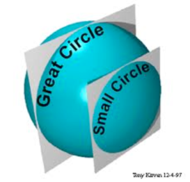
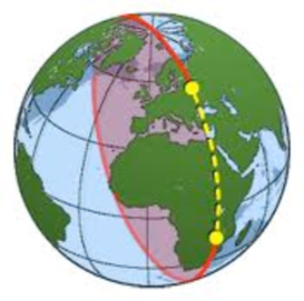
A great circle (geodesic)	A geodesic minimum and a geodesic saddle point

Figure 5: Geodesics on the sphere are arcs of great circles

A sphere is one simple and interesting example of a curved surface. Suppose that SPC travels along the equator of the earth. This path is completely unchanged by replacing the sphere with its mirror image around the equator, so the left and right wheel travel the same distance and the statue does not rotate. The equator is a geodesic! By the same reasoning, any circle which cuts the sphere into two identical halves is a geodesic, as in Figure 5. Such circles, whose centers coincide with the center of the sphere, are called “great circles.” Airplane pilots know this – when they travel between two points far apart on the earth, they plot a path that follows the great circle connecting them (again the analogy with straight lines, and Euclid’s remarkable prescience, are affirmed: Two points generally determine a great circle!), because they know that this will be the shortest distance. However, while traveling on a great circle from Moscow to Dar es Salaam over the Mediterranean is a geodesic and gives the shortest path between these two points, traveling the opposite way on the same great circle (similar to the path traveled in red in Figure 5) is still a geodesic but is definitely not the shortest route to Dar es Salaam from Moscow, similar to the right side of Figure 5. Geodesics are not always minima of distance. In fact, since such nonminimal geodesics can be perturbed in certain directions to make the distance smaller and in certain directions to make the distance larger, they are infinite-dimensional analogues of the saddle points of multivariable calculus.

Taking the analogy between lines on a plane and great circles on a sphere in complete earnest, compare Euclid’s geometry of triangles and parallel lines to their analogues on a sphere. (Some fine print: Two points on a sphere determine a great circle unless they are antipodal. Students of spherical geometry handle this embarrassment by treating pairs of antipodal points as a single point, an issue we can safely ignore [McC13, Pol]) For example, suppose that SPC travels due west from some point on the equator one quarter of the way around the earth, then due north straight to the north pole, and then turns $\pi/2$ radians and heads due south back to its starting point. This closed path made of three geodesics is called a triangle in spherical geometry. But this triangle has three internal right angles, something that could never happen in plane geometry, where the sum of the internal angles of a triangle is always $\pi.$ In this case the sum is $3\pi/2,$ which is $\pi/2$ too many. Euclid’s sum of angles theorem does not hold on the sphere – it turns out that this is the case because it relied on the parallel line postulate.

If the statue starts out pointing in the traditional south direction, it points straight to the left on the first leg of the journey, directly behind on the second, and straight to the right on the third leg, so it ends up pointing due west. This is more proof that SPC fails as a navigational aid – not only does it fail to point south under certain circumstances, it does not even return from a journey pointing in the same direction as it started! But the $\pi/2$ which it rotated in its journey and the $\pi/2$ by which the sum of the angles exceeds the expected sum are related, perhaps not surprisingly.

Draw a few triangles on a sphere, make a rough estimate of both the angle sum and the amount that SPC rotates as it traverses the triangle, and some guesses may present themselves. The angle sum always exceeds the expected $\pi,$ the amount it exceeds it by is always the amount that the SPC rotates (clockwise) over the journey, and this amount seems to be roughly proportional to the size of the triangle. If you do not have a south pointing chariot on hand, you are just estimating the quantity crudely, and I could not expect you to observe anything more precise than “the bigger the triangle the more the rotation.” But notice that a tall, very thin triangle has two almost right angles and one almost $0$ angle, so this rotation is still quite small. That suggests that the right measure of the size of the triangle is the area, not, say, its longest dimension.

Figure 6: SPC gets very confused traversing this triangle

This observation is not unique to triangles. The general statement on the plane is that the sum of the external angles of a polygon is always $2\pi.$ On a sphere, the sum of the external angles of a polygon (a closed curve made up of pieces of great circles) will always be less than $2\pi,$ and less by the exact amount that the SPC rotates as it traverses that polygon, a quantity that will in fact be exactly proportional to the area of the figure encompassed [McC13, Pol].

All of this empirical exploration suggests that when SPC travels in a loop, the total rotation it undergoes between the start and the finish is some measure of how the surface curves in the interior of the region subsumed by the loop. This is correct, and the rest of this article is devoted to convincing you that this is correct, and exploring the outsized consequences of this one fact.

5 Holonomy

To understand what is going on requires a little abstraction. For each loop $L$ (a path that begins and ends at the same point) on some surface, let $H(L),$ the “holonomy” of the loop, be the rotation that the pointer on SPC undergoes in traversing that loop (make sure you are convinced that the amount that the pointer rotates is not affected by where the pointer started). Holonomy views this rotation as a function on the set of all possible loops.

Here the narrative must pause again for a technicality. The angle $2\pi$ is the same angle as the angle $0.$ But if you have ever walked a rambunctious dog on a leash, you know that when the dog has run $2\pi$ radians around you, while she is in the same position as if she had stayed still, your leash can tell the difference. If you were riding on SPC, and you slept through the journey, you would only know the angle of the final position compared to the original angle. But if you were awake and watching the statue rotate (or tied a string to the statue’s finger) you would know the total rotation, and would be able to distinguish a $0$ rotation from a $2\pi$ rotation from a $4\pi$ rotation. Thus with care one can think about the holonomy not just as an angle, but as a real number, with differences of $2\pi$ being meaningful. This distinction will only matter near the very end, and can be ignored with little loss of comprehension.

To understand a function as a tool, a mathematician first asks how the function responds to natural operations on its domain. One natural operation on loops is really an operation on the larger set of all paths. If the path $B$ begins at the point where the path $A$ ends, then it is natural to define the composition of the two paths $B\circ A,$ which traces the path $A$ and then the path $B.$ If two loops $L_{1}$ and $L_{2}$ have the same base point (the common starting and ending point), then the composition $L_{1}\circ L_{2}$ is a loop (you understand this definition if you can convince yourself that composition is not commutative, i.e. that for some loops $L_{1}\circ L_{2}\neq L_{2}\circ L_{1}$).

So what is the holonomy of $L_{2}\circ L_{1}$ in terms of the holonomy of $L_{1}$ and the holonomy of $L_{2}?$ If you are the kind of person who flips to the last page of a mystery novel rather than trying to work it out yourself, resist the desire and take a moment to think it through before proceeding. Picture it rotating $30^{\circ}$ as it traverses $L_{1}$ and $20^{\circ}$ as it traverses $L_{2}$. Then if it traverses the first loop followed by the second it will rotate … $50^{\circ}.$ In general

$$H(L_{2}\circ L_{1})=H(L_{2})+H(L_{1}).$$

Think of this property as saying that holonomy turns the composition operation on loops into the addition operation on numbers. When a function turns the natural operation in the domain into the natural operation in the range, it is called a homomorphism, and this is one of the nicest properties a function can have, according to a mathematical aesthetic.

Figure 7: Composition of two loops

The second property is a bit subtler. Suppose that SPC traverses a loop $L,$ and somewhere in the middle of it turns off the loop, travels along some path to a different destination, then returns on the same path to where it left the loop, and continues the rest of the way along the loop, as in Figure 7. Call this enhanced loop $L^{\prime}$ and refer to it as a detour. How are $H(L)$ and $H(L^{\prime})$ related? When SPC turns off its original path, it turns, say, $\theta$ radians clockwise, and therefore the left wheel advances $w\theta/2$ and the right wheel $-w\theta/2.$ Then SPC travels along the detour,and the left and right wheel each advance by some unknowable amount. At the terminus of the detour, SPC turns around $\pi$ radians, lets say counterclockwise, so the right wheel advances $w\pi/2$ and the left wheel advances $-w\pi/2.$ Returning on the detour path in the opposite direction, notice that the left wheel now travels exactly the distance the right wheel had on the outbound journey, and vice versa. So the total distance traveled by each wheel from these two legs is exactly the same, and thus has no effect on the rotation of the statue. Finally, upon returning to the original loop, SPC must rotate $\pi-\theta$ clockwise to return to its original direction. Adding up all the left and right wheel distances, you see that they are equal, and SPC has not rotated a bit for all that effort. From this conclude

$$H(L)=H(L^{\prime}),$$ (5.1)

that is to say adding a detour in this sense to any loop has no effect on the holonomy.

Figure 8: A loop with a detour, and the tracks of SPC

Perhaps you noticed a subtlety in the above argument. At the end of the detour SPC turned around in the counterclockwise direction, but might just as well have chosen to turn in the clockwise direction. Had it done so, a careful accounting shows that the statue would have added one extra counterclockwse rotation of $2\pi$ during the detour. To compute only the angle of holonomy, this is of no account, but in terms of the numerical holonomy, Eq. (5.1) is true only if SPC does its about-faces correctly. Specifically, whatever direction SPC turns to get on and off the detour, it must turn the opposite way at the extreme point of its detour.

There is a second case involving a detour move. The stereotypical American way to exercise is to drive to the running track, run around the track, and then drive home. Here the loop $L$ is the run around the track, and the longer loop $L^{\prime}$ is the loop $L$ bracketed by a path and its reverse at the beginning and end of the loop. So now $L$ and $L^{\prime}$ have different starting points, but repeating the logic it is still true that $H(L^{\prime})=H(L).$ Once again for numerical holonomy attention must be paid to the direction of rotations.

So holonomy assigns a number or angle to each loop in such a way that composition of loops turns into addition and detours have no effect. These two properties are already enough to make a key observation. Imagine that the loop SPC travels on a loop surrounding a region. You may not have imagined that there was any other possibility, but if the surface were the surface of a doughnut, for instance, what mathematicians call a torus, the loop could wrap around the doughnut as if it were a ribbon wrapped around a gift. Instead assume that the loop surrounds a region $R.$ First notice that the holonomy is the same regardless of what point is the start and end of the loop, because the effect of starting and ending at a different point is exactly a detour move of the second kind. So define the holonomy of the region $R$ to be the holonomy of any loop $L$ that goes once clockwise around the region. This does not specify the loop uniquely, but does specify the holonomy.

Now divide $R$ into two regions $R_{1}$ and $R_{2}.$ Let $x$ be a point on their shared boundary, let $L_{1}$ be the loop that goes clockwise around $R_{1}$ based at $x,$ and let $L_{2}$ be the loop that goes clockwise around $R_{2}$ based at $x$ as in Figure 9. Notice that $L_{2}\circ L_{1}$ is a detour of $L.$ Thus $H(L)=H(L_{1})+H(L_{2})$ so the holonomy of $R$ is the sum of the holonomies of $R_{1}$ and $R_{2}.$ This argument generalizes to say that the holonomy of any region divided into subregions is the sum of the holonomies of the subregions. Holonomy behaves like area, in that the whole is equal to the sum of its parts.

Figure 9: Cutting a region into pieces

The last thing I need you to believe about holonomy puts the most demand on your visual intution. The rough idea is that holonomy should be continuous, that small changes to the loop should cause small changes in the holonomy. In particular if you move a small loop from a flat area to a steep hill, you would not be surprised if the holonomy changed a lot, but if you moved a small loop at one point on a hill to a similarly shaped small loop at a nearby point, near enough that the “roundness” or “curvature” of the hill has not changed much, you would expect the holonomy to change very little.

Now consider four nearby points on the surface, arranged so as to form an approximate rectangle, i.e. so that when they are connected by geodesics all four angles are close to right angles. Let $R$ be the interior of this rectangle and consider the quantity

$$\frac{H(R)}{\text{Area}(R)}.$$

By dividing two opposite edges into $n$ equal length intervals and the other pair of opposite edges into $m$ equal intervals, we divide the entire approximate rectangle into $nm$ approximate rectangles that are all of approximately the same shape and size. So, it should be plausible that their holonomies are all approximately equal and that their areas are all approximately equal. Since both holonomies and areas add, calling one of the smaller rectangles $R_{1}$ we have that

$$\frac{H(R)}{\text{Area}(R)}\sim\frac{nmH(R_{1})}{nm\text{Area}(R_{1})}=\frac{H(R_{1})}{\text{Area}(R_{1})}.$$

The approximation gets better the smaller the size of the rectangle, so imagine a sequences of rectangles $R_{n}$, whose sizes approach zero and which all surround one point $x.$ This heuristic argument suggests that the limit of the ratio of holonomy to area converges for this sequence, which in fact it does. Define the curvature $K(x)$ of the surface at the point $x$ to be this limit

$$\lim_{n\to\infty}\frac{H(R_{n})}{\text{Area}(R_{n})}=K(x).$$

In fact, by varying $n$ and $m$ it should also be plausible that this number does not depend on the shape of the sequence of rectangles.

Below I will argue that this real-valued function $K(x)$ defined on the surface does a good job of measuring your intuitive notion of how curved the surface is at each point. But first a remarkable fact: Another way to express this limit is to say that for such a rectangle the holonomy is approximately equal to the area times the curvature of some point in the interior. Imagine an arbitrary region, but still small, so that we can draw a sequence of geodesics on it that divide the region up into many small rectangles (this requires replacing the boundary with a more jagged approximation). For the $i$th approximate rectangle, call the side lengths $\Delta x_{i}$ and $\Delta y_{i},$ and let $K(x_{i},y_{i})$ be the curvature of some point in the rectangle, so that the holonomy of that rectangle should be approximately

$$K(x_{i},y_{i})\Delta x_{i}\Delta y_{i}$$

as in Figure 10 In particular the holonomy of the entire region should be approximated by

$$\sum_{i}K(x_{i},y_{i})\Delta x_{i}\Delta y_{i}.$$

Of course here when we say approximate we are including errors that come from approximating the region by these (approximate) rectangles, from approximating the area by $\Delta x_{i}\Delta y_{i},$ and from approximating the holonomy by area times the curvature at one point. Your trust is required to believe that as the region is divided more finely all these errors go to zero rapidly enough that

$$H(R)=\lim_{\Delta x_{i},\Delta y_{i}\to 0}\sum_{i}K(x_{i},y_{i})\Delta x_{i}\Delta y_{i}.$$

Figure 10: Chopping into small rectangles

But granting this much trust, then all that is required of you is recollection. You have seen (at least if you have taken multivariable calculus before) this limit. It is exactly how the integral of a function over a two dimensional region is defined. The conclusion is that the holonomy around a closed loop that surrounds a region $R$ is the integral of curvature over $R,$ or

$$H(R)=\iint_{R}K(x,y)dxdy.$$

On the one hand, this is a really remarkable claim. If SPC goes on a long trip around northern Arizona, this says that the position of the flag at the end depends on the value of curvature at each point that its path surrounds. If the path encloses the Grand Canyon, where one presumes the curvature function would vary wildly, the position of the flag will in some sense record information about this curvature at each point in the canyon, even though from the SPC one might never have seen the Grand Canyon. On the other hand, this result looks superficially very similar to, and indeed is deeply connected to, results like the Divergence Theorem and Green’s Theorem, which relate an integral along a closed path to a higher dimensional integral of something else over the interior (note in paragraph 4 of Section 2 that the rotation of the pointer is calculated by an integral).

Let’s explore what this notion of curvature looks like with some examples.

6 Exploring the Earth II

The curvature at a give point on the sphere is given by the limit of the ratio of the holonomy around the rectangle to the area of the rectangle as the size of the rectangle goes to zero. Consider such a decreasing sequence of smaller rectangles at some point $p$ on the sphere, and suppose that $q$ is a different point on the sphere. Then there is a rotation of the sphere that takes $p$ to $q,$ which therefore takes that sequence to a sequence of decreasing rectangles around $q.$ Because a rotation of the sphere will clearly preserve all distances, angles and areas, the resulting loops will still be approximately rectangular and will have the same area and holonomy. Thus the ratio will converge to the same thing, so that the curvature at every point of the sphere must be the same. This makes perfect sense: The sphere is maximally symmetric, so a reasonable measure of the curvature at each point should be preserved by all those symmetries.

In Section 4 the holonomy of the loop pictured in Figure 6 was computed to be $\pi/2.$ This holonomy is equal to the integral of the curvature function over the interior of the triangle $\int\int_{R}K(p)dp.$ However, since the curvature is a constant $K,$ the holonomy is $K\text{Area}(R).$ The area of this region is $1/8$ of the area $4\pi r^{2}$ of the sphere, from which it follows that the curvature at each point of a sphere of radius $r$ is $1/r^{2}.$ This very simple formula should make intuitive sense. A large radius sphere, like the earth, is almost flat, while a very small radius sphere is extremely curved.

Similarly, a small rectangle on the cylinder with two sides parallel to the axis of rotation and two sides perpendicular to it can be translated up and down the axis and rotated around it to a rectangle with the same angles anywhere on the cylinder. So by the same reasoning, the cylinder has constant curvature. But in this case the small rectangle made up of geodesics has four right angles, which means that its angle deficit is zero and therefore the curvature of the cylinder is $0.$ The cylinder, if you will, is flat. This quite likely does not fit so well with your intuitive notion of curvature.

In fact there is more than one intuitive notion of curvature that we tend to mix up. If you deform a surface so that all the distances on it remain unchanged, you have not changed its curvature in this sense. To make this somewhat technical notion a little more concrete, consider a piece of cloth. Draw a path on the piece of cloth and then bunch it up. You’ve deformed the piece of cloth, but the path length has not changed, because that would require stretching the fabric. If lengths of paths and therefore distances are unchanged by anything you can do to (idealized) cloth, then the amount SPC rotates along a path is also unchanged, since it only depends on the distances each wheel travels. Thus holonomy and curvature are unchanged by such a deformation. We speak of “intrinsic geometry” to refer to any property of a surface that is unchanged by a deformation you can do to cloth without stretching it. That is to say, a deformation that does not change the lengths of any paths.

A flat piece of cloth can be wrapped around a cylinder without stretching any part of it. So a cylinder has the same intrinsic geometry as a flat plane, and in particular has the same curvature. The kind of bending that turns the flat cloth into a cylinder does not change its intrinsic geometry and “does not count” as far as curvature is concerned.

Which brings us at last to the point.

7 Mapping the Earth

The standard Mercator projection (Figure 11) does not represent distances accurately. It makes Canada, Russia, and Antarctica look immense, while equally big regions near the equator look small. Obviously this is a poor property for a map to have. Various schemes attempt to solve this problem, but can they? Is it possible to draw a map of the world on which all distances are represented proportionally? Another form of the question asks if one can peel an orange so that the skin can be laid flat without stretching. Note that you are allowed to cut the skin in various places, as in Figure 11. Nevertheless the answer is no.

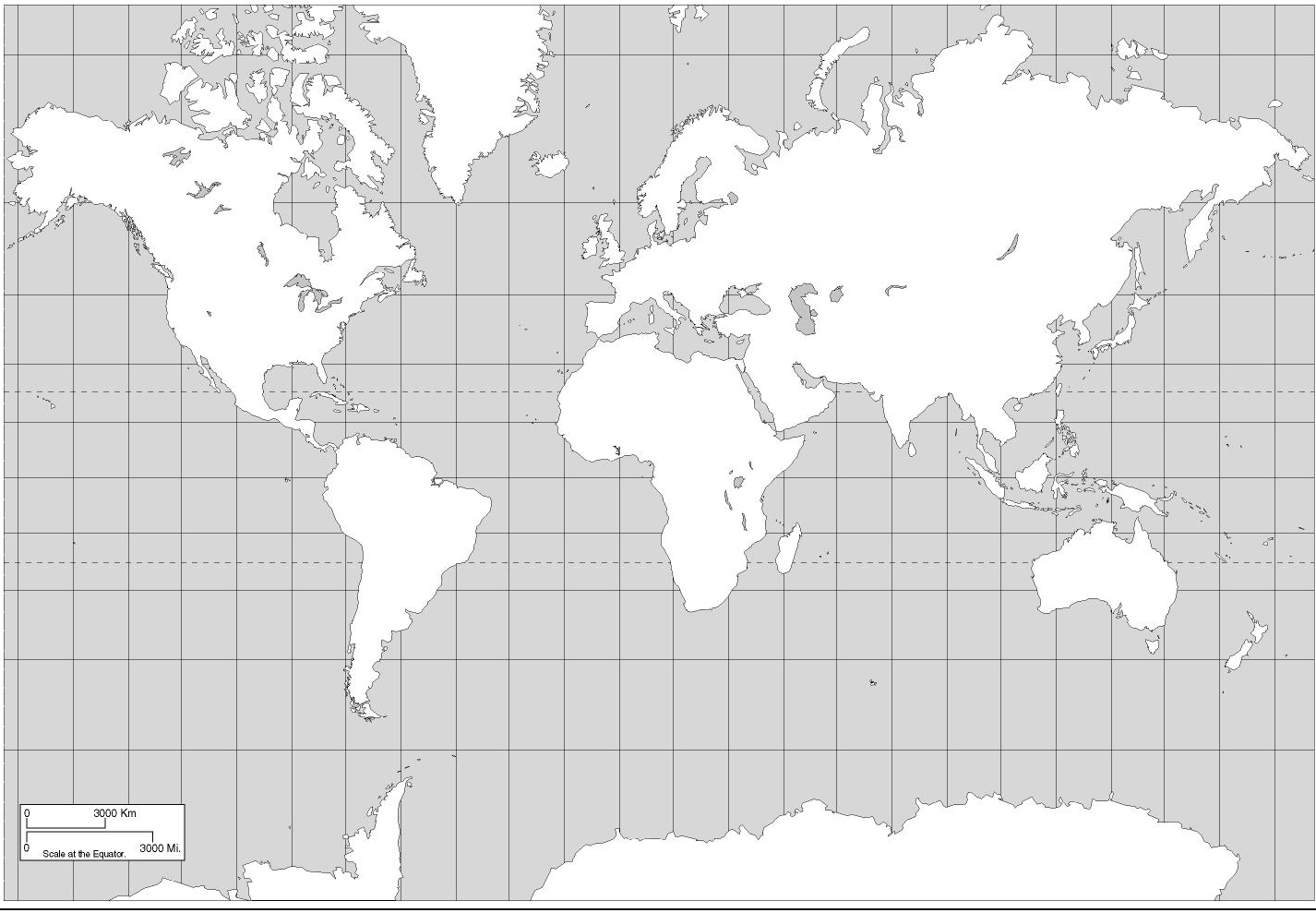
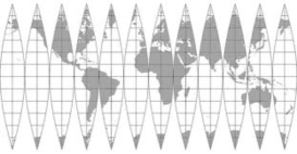
Figure 11: Mercator and a competing projection of the earth

The reason is clear from our previous discussion. If the identification between the earth and the map preserved distances, then since the workings of SPC only depend only upon distances, every loop on the earth must have the same holonomy as the corresponding loop on the map. But the holonomy of a loop on the earth will be proportional to the area enclosed, whereas the holonomy of a loop on a flat map is necessarily zero. So such a map is impossible!

8 Gauss’ Theorema Egregium and Beyond

This notion of curvature, and the many things it tells you, including the fact about maps of the earth, are due to Gauss. Gauss did not describe curvature in terms of south pointing chariot. Gauss gave a definition of the curvature that depends on how the surface is embedded in three space. Roughly Gauss imagines rotating and moving the surface in three dimensions until the desired point on the surface is at the origin and the tangent plane at that point is the $xy$ plane. At least near the origin the surface can then be written in the form $z=f(x,y),$ where the Taylor series expansion of $f$ has no constant or linear terms. A further rotation about the $z$ axis guarantees that

$$f(x,y)=ax^{2}+by^{2}+\,\text{third order and higher}.$$

Gauss’ curvature is simply $4ab.$ Gauss was then able to prove that although this definition clearly depends on the details of how the surface is embedded in three space, the resulting curvature does not, and only depends on the distances within the surface, that is on its intrinsic geometry [McC13]. Gauss found this result so surprising that he called it his “Theorema Egregium” or “Remarkable Theorem.” If you are familiar with even a few of the revolutionary results which are due to Gauss (several of them simply called Gauss’ Lemma), you will understand that this is quite a statement.

Our definition of curvature is based on the SPC which is manifestly intrinsic, and thus seems to have avoided the work of the Theorema Egregium. Of course this is because we skipped over hard analytic issues, and in particular relied on nothing but the reader’s trust for the existence of the limit (and rate of convergence) of the definition of curvature.

Gauss’ work has been extended in several directions. Most importantly, all this can be done with great care in more dimensions than two (replace SPC with a rocket ship with a gyroscope), where the notion of curvature and holonomy are quite a bit more complicated (one must keep track of the change in the path’s length as you perturb it in each direction). SPCs doomed attempt to keep track of a global direction (towards the south pole) with a local calculation (the gears and the distances its wheels travel) is using the mathematical notion of parallel transport [San92], which can be generalized beyond distances to mathematical objects called connections. Connections are used to model all of the fundamental forces of nature except gravity (it plays a role in modeling gravity as well) and, in some reckonings, even monetary inflation! These ideas are the building blocks of differential geometry.

References

- [FO] José Figueroa-O’Farrill. Brief notes on the calculus of variations. http://www.maths.ed.ac.uk/ jmf/Teaching/Lectures/CoV.pdf.
- [McC13] John McCleary. Geometry from a differentiable viewpoint. Cambridge University Press, Cambridge, 2 edition, 2013.
- [NL65] Joseph Needham and Wang Ling. Science and Civilisation in China, volume 4. Cambridge University Press, 1965.
- [Pol] John C. Polking. The geometry of the sphere. http://math.rice.edu/ pcmi/sphere/.
- [San92] M. Santander. The Chinese south‐seeking chariot: A simple mechanical device for visualizing curvature and parallel transport. American Journal of Physics, 60(782), 1992.
- [ST67] I. M. Singer and John A. Thorpe. Lecture Notes on Elementary Topology and Geometry. UTM. Springer-Verlag, New York, 1967.
- [Wei74] Robert Weinstock. Calculus of Variations. Dover Publications, New York, 1974.