Optomechanical creation of magnetic fields for photons on a lattice

Abstract

We propose using the optomechanical interaction to create artificial magnetic fields for photons on a lattice. The ingredients required are an optomechanical crystal, i.e. a piece of dielectric with the right pattern of holes, and two laser beams with the right pattern of phases. One of the two proposed schemes is based on optomechanical modulation of the links between optical modes, while the other is a lattice extension of optomechanical wavelength-conversion setups. We illustrate the resulting optical spectrum, photon transport in the presence of an artificial Lorentz force, edge states, and the photonic Aharonov-Bohm effect. Moreover, we briefly describe the gauge fields acting on the synthetic dimension related to the phonon/photon degree of freedom.

Light interacting with nano-mechanical motion via the radiation pressure force is studied in the field of optomechanics. The field has seen rapid progress in the last few years (see the recent review Aspelmeyer2013RMPArxiv ). So far, most experimental achievements have been realized in setups comprising one optical mode coupled to one vibrational mode. Obviously, one of the next frontiers will be the combination of many such optomechanical cells into an optomechanical array, enabling the optical in-situ investigation of (quantum) many-body dynamics of interacting photons and phonons. Many experimental platforms allow to be scaled up to arrays. However, optomechanical crystals seem to be the best suited candidate at the present stage. Optomechanical crystals are formed by the periodic spatial patterning of regular dielectric and elastic materials, resulting in an enhanced coupling between optical and acoustic waves via moving boundary or electrostriction radiation pressure effects. Two-dimensional (2D) optomechanical crystals with both photonic and phononic bandgaps Safavi-Naeini2010 can be fabricated by standard microfabrication techniques through the lithographic patterning, plasma etching, and release of a thin-film material Eichenfield2009 . These 2D crystals for light and sound can be used to create a circuit architecture for the routing and localization of photons and phonons Eichenfield2009 ; Safavi-Naeini2010APL ; Gavartin2011PRL_OMC ; Chan2011Cooling ; SafaviNaeini2014SnowCavity .

Optomechanical arrays promise to be a versatile platform for exploring optomechanical many-body physics. Several aspects have already been investigated theoretically, e.g. synchronization Heinrich2011CollDyn ; Holmes2012 ; Ludwig2013 , long-range interactions Bhattacharya2008 ; Xuereb2012 , reservoir engineering Tombadin2012 , entanglement Schmidt2012 ; Akram2012 , correlated quantum many-body states Ludwig2013 , slow light Chang2011 , transport in a 1D chain Chen2014 , and graphene-like Dirac physics Schmidt2014 . .

One of the central aims in photonics is to build waveguides that are robust against disorder and do not display backscattering. Recently there have been several proposals Koch2011 ; Hafezi2011 ; Umucallar2011 ; Fang2012 ; Hafezi2012OptExpr to engineer non-reciprocal transport for photons. On the lattice, this corresponds to an artificial magnetic field,which would (among other effects) enable chiral edge states that display the desired robustness against disorder. First experiments have shown such edge states Hafezi2013 ; Mittal2014 ; Rechtsman2013Nat . These developments in photonics are related to a growing effort across various fields to produce synthetic gauge fields for neutral particles Bermudez2011 ; Aidelsburger2013 ; Miyake2013 .

In this paper we will propose two schemes to generate an artificial magnetic field for photons on a lattice. In contrast to any previous proposals or experiments for photonic magnetic fields on a lattice, these would be controlled all-optically and, crucially, they would be tunable in-situ by changing the properties of a laser field (frequency, intensity, and phase pattern). They require no more than a patterned dielectric slab illuminated by two laser beams with suitably engineered optical phase fields. The crucial ingredient is the optomechanical interaction.

On the classical level, a charged particle subject to a magnetic field experiences a Lorentz force. In the quantum regime, the appearance of Landau levels leads to the integer and fractional quantum Hall effects, where topologically protected chiral edge states are responsible for a quantized Hall conductance. On a closed orbit, a particle with charge $q$ will pick up a phase that is given by the magnetic flux $\Phi$ through the circumscribed area, where $\Phi=(q/\hbar)\int{\bf B}\cdot d\mathbf{S}$ in units of the flux quantum, with ${\bf B}$ denoting the magnetic field. On a lattice, a charged particle hopping from site i to j acquires a Peierls phase $\phi_{ij}=(q/\hbar)\int_{{\bf r}_{i}}^{{\bf r}_{j}}{\bf A}d{\bf r}$ determined by the vector potential ${\bf A}$. Conversely, if we can engineer a Hamiltonian for neutral particles containing arbitrary Peierls phases,

$$\hat{H}_{\text{hop}}=\hbar J\sum_{\langle ij\rangle}e^{i\phi_{ij}}\hat{a}_{j}^{\dagger}\hat{a}_{i}+\text{h.c.},$$ (1)

we are able to produce a synthetic magnetic field. Here $\hat{a}_{i}$ is the (bosonic) annihilation operator on lattice site i. We note in passing that different phase configurations can lead to identical flux patterns, reflecting the gauge invariance of Maxwell’s equations under the transformation ${\bf A}\rightarrow{\bf A}+\nabla\xi({\bf r})$ for any scalar function $\xi$.

Every defect in an optomechanical crystal Eichenfield2009 ; Safavi-Naeini2010APL ; Gavartin2011PRL_OMC ; Chan2011Cooling ; SafaviNaeini2014SnowCavity supports a localized vibrational (annihilation operator $\hat{b}$, eigenfrequency $\Omega_{0}$) and optical mode ($\hat{a}$, frequency $\omega_{\text{cav}}$) that interact via radiation pressure, giving rise to the standard optomechanical interaction Aspelmeyer2013RMPArxiv :

$$\hat{H}_{\text{int}}=-\hbar g_{0}\hat{a}^{\dagger}\hat{a}(\hat{b}^{\dagger}+\hat{b}).$$ (2)

This can be utilized in two basic ways to introduce phases for the hopping of photons. First, one can drive the optical mode by a control laser (frequency $\omega_{L}$) close to the red sideband, $\omega_{L}\sim\omega_{\text{cav}}-\Omega_{0}$. Following the standard procedure of linearization and rotating wave approximation (RWA) Aspelmeyer2013RMPArxiv one recovers a swap Hamiltonian, $g\hat{a}^{\dagger}\hat{b}+\text{h.c.}$, in which the phase $\phi$ of the coupling $g\in\mathbb{C}$ is set by the control laser phase. We will show below how this can be used to create a photonic gauge field. There is, however, also a second route, namely, driving the vibrational mode into a large amplitude coherent state, $\langle\hat{b}(t)\rangle=|\beta|e^{-i(\Omega t+\phi)}$, using the radiation pressure force. These oscillations then weakly modulate the optical eigenfrequency, $\omega_{\text{cav}}(t)=\omega_{\text{cav},0}+2g_{0}|\beta|\cos(\Omega t+\phi)$, with the phase $\phi$ set by the oscillations. Again, in a suitable setting this will lead to an artificial magnetic field for the photons. We now describe both methods in turn.

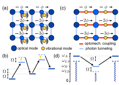
Figure 1: Proposed schemes to create a photonic gauge field in optomechanical arrays by engineering photon hopping phases. (a) Modulated link scheme. (b) Corresponding optical spectrum of a row with relevant sidebands (dashed). Driven vibrational modes (yellow) optomechanically modulate the frequency of optical link modes. Tunneling photons are thus up-converted to the first sideband and pick up the phase of the modulation. Arrows in (b) indicate the resonant photon transmission process in a row. (c) Wavelength conversion scheme and (d) corresponding optical spectrum: Neighboring modes in a row couple to a vibrational mode (yellow) optomechanically (red lines, denoting the linearized optomechanical interaction). Two lasers, driving the optical modes close to the red sidebands (wiggly arrows in d), give rise to resonant photon-phonon-photon conversion with the phase set by the lasers. Different rows are connected via simple photon hopping (blue lines), without a phase, in both schemes (a,c). The indicated phase configuration corresponds to a constant magnetic field.

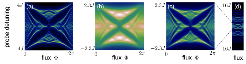
Figure 2: Comparison between the experimentally accessible optical spectrum (LDOS) of the ideal effective Hofstadter model (a) and the actual results from the proposed modulated link scheme (b-d), for different optical decay rates and magnetic fluxes. The simulation results indicate that the scheme works even beyond the perturbative regime. The resulting Hofstadter butterfly could be observed by a local tapered fiber probe. Modulation of links produces higher side bands (d). The phase configuration corresponds to a constant magnetic flux $\Phi$ per plaquette, see Fig. 1. [Parameters: grid: 10x10 (a), 12x12 (b-d); $J_{\text{eff}}=0.108\Omega_{0}$ (a-d); $\kappa=0.01\Omega_{0}$ (a,c,d), $\kappa=0.05\Omega_{0}$ (b); $J=0.3\Omega_{0}$ (b-d); $g_{0}|\beta|=0.3\Omega_{0}$ (b-d); optical eigenfrequencies (relative to first mode) in a row (left to right) including interface modes: $(0,0.5,1,1.5,\dots)\Omega_{0}$ (b-d).]

Modulated link scheme. – Recently Fang et. al. Fang2012 ; Tzuang2014 proposed to create a photonic gauge field by electro-optically modulating the photon hopping rate $J_{ij}=J\cos(\Omega t+\phi_{ij}$) between neighboring cavities. This would require locally wired electrodes for each link of the lattice. Here we propose a potentially more powerful all-optical implementation of that idea. We employ optomechanically driven photon transitions, as first discussed in Heinrich2010_Landau , but extended to a scheme with modulated interface modes, depicted in Figure 1 (a). We now discuss the leftmost three optical modes in the first row, $\hat{a}_{A}$, $\hat{a}_{I}$, $\hat{a}_{B}$ (from left to right), exemplary of the full grid. Their coherent dynamics is governed by the Hamiltonian

$$\hat{H}/\hbar=\sum_{i=A,B}\omega_{i}\hat{a}_{i}^{\dagger}\hat{a}_{i}+\omega_{I}(t)\hat{a}_{I}^{\dagger}\hat{a}_{I}-J(\hat{a}_{I}^{\dagger}\hat{a}_{A}+\hat{a}_{B}^{\dagger}\hat{a}_{I}+\text{h.c.}).$$ (3)

The terms describe, in this order, the first (A) and third (B) optical mode, the temporally modulated interface mode (I), and its tight binding coupling to the neighboring A and B modes with photon tunneling rate $J$. As discussed further below, the eigenfrequency $\bar{\omega}_{I}$ of the interface mode should be well separated from the eigenfrequencies of the adjacent A and B modes, for the transition $A\text{\textendash I\textendash B}$ to be virtual. The interface mode is optomechanically coupled to a mechanical mode, which itself is driven into a large amplitude coherent state. As mentioned above, this gives rise to a weak modulation of its optical eigenfrequency, $\omega_{I}(t)=\bar{\omega}_{I}+2g_{0}|\beta|\cos(\Omega t+\phi)$, with the phase $\phi$ set by the driving. The required mechanical driving is easily generated by two-tone laser excitation at a frequency difference $\Omega$. The beating between the laser beams gives rise to a sinusoidal radiation pressure force, which drives the mechanical mode. If $\omega_{B}=\omega_{A}+\Omega$, then a photon hopping from site A to B picks up the phase $\phi$ of the modulation: Starting from $\hat{a}_{A}$, it tunnels into $\hat{a}_{I}$ where it is inelastically up-scattered into the first sideband by the modulation and subsequently tunnels into $\hat{a}_{B}$ resonantly, as shown by the spectrum in Figure 1(b). We can derive an effective Hamiltonian, $\hbar J_{{\rm eff}}e^{i\phi}\hat{a}{}_{B}^{\dagger}\hat{a}{}_{A}+\text{h.c.}$ for this process by integrating out the interface mode $I$ using Floquet perturbative methods to third order (see Appendix A). For the effective hopping rate we find $J_{{\rm eff}}=g_{0}|\beta|J^{2}/[(\omega_{A}-\omega_{I})(\omega_{B}-\omega_{I})]$, to leading order in $J$ and $\left|\beta\right|$. Concatenating such three-mode blocks, we create a linear chain (the first row in Figure 1a), with its optical spectrum schematically depicted in Figure 1(b). Every time a photon hops to the right, it is up-converted and picks up the phase of the drive. To obtain a 2d grid, we stack identical chains and connect neighboring rows by direct photon hopping (whose rate must be chosen to equal $J_{\text{eff}}$, to obtain isotropic hopping), as depicted in Figure 1(b). The phase configuration in Figure 1(a) corresponds to a constant magnetic field. Note that in contrast to the general Hamiltonian (1), this scheme does not allow for phases when hopping between rows, yet it is still possible to achieve an arbitrary flux through every plaquette. Hence, arbitrary magnetic fields can be generated, provided one can control the driving laser phase at every interface mode. With the help of wave front engineering, this can be achieved with no more than two lasers: A homogeneous ’carrier’ beam $E_{1}=E_{10}e^{-i\omega_{L}t}$ and a ’modulation’ beam $E_{2}=E_{20}e^{-i(\omega_{L}+\Omega)t-i\phi(x,y)}$, with an imprinted phase pattern $\phi(x,y)$. Interference yields the desired temporally modulated intensity $\left|E_{10}\right|^{2}+\left|E_{20}\right|^{2}+2{\rm Re}[E_{10}^{*}E_{20}e^{-i(\omega_{{\rm L}}t+\phi(x,y))}]$, exerting a radiation force with a site-dependent phase. Care has to be taken to avoid exciting other vibrational modes (those not at the interface mode), by engineering them to have different mechanical frequencies. To this end, the driving frequency $\Omega$ would usually be chosen close to the mechanical eigenfrequency $\Omega_{0}$, so the mechanical amplitude is enhanced by the mechanical quality factor and is thus much larger than any spurious amplitude in other (off-resonant) modes. By engineering the intensity pattern $|E_{20}(x,y)|$ as well, one could suppress any such unwanted effects even further.

Wavelength conversion scheme. - There is another, alternative way of engineering an optical Peierls phase, and it is related to optomechanical wavelength conversion Hill2012WavelengthConversion ; Dong2012 . In wavelength conversion setups, low frequency photons in one mode are up-converted to a higher frequency in another mode by exploiting the modes’ mutual optomechanical coupling to a vibrational mode. We propose to scale up this idea into a grid as depicted in Figure 1(c). The leftmost three modes in the first row depict (in this order) an optical mode (annihilation operator $\hat{a}_{A}$, frequency $\omega_{A}$), a mechanical mode ($\hat{b}$, $\Omega_{0}$) and another optical mode ($\hat{a}_{B}$, $\omega_{B}\neq\omega_{A}$). The mechanical mode couples optomechanically to both optical modes. A and B are driven by a laser with frequency $\omega_{L1}$ and $\omega_{L2}$, respectively: For mode $A$, we require $\omega_{A}-\omega_{L1}=\Omega_{0}+\delta\equiv\Omega$ where $\omega_{L1}$ denotes the driving laser’s frequency and $\delta\ll\Omega_{0}$ is the detuning from the red sideband. For mode $B$, a similar relation $\omega_{B}-\omega_{L2}=\Omega$ holds, as depicted in the spectrum in Figure 1(d). After application of the standard linearization and RWA procedure Aspelmeyer2013RMPArxiv , the dynamics in a frame rotating with the drive is governed by the Hamiltonian

$$\hat{H}/\hbar=\Omega\sum_{i=A,B}\hat{a}_{i}^{\dagger}\hat{a}_{i}+\Omega_{0}\hat{b}^{\dagger}\hat{b}-(g_{A}^{*}\hat{a}_{A}\hat{b}^{\dagger}+g_{B}\hat{a}_{B}^{\dagger}\hat{b}+\text{h.c.}).$$ (4)

Elimination of the mechanical mode leads to an effective Hamiltonian $\hbar J_{\text{eff}}e^{i\phi}\hat{a}_{B}^{\dagger}\hat{a}_{A}+\text{h.c.}$ to leading order in $|g_{A,B}|/\delta$, with effective hopping rate $J_{\text{eff}}=|g_{A}||g_{B}|/\delta$ and hopping phase $\phi=\phi_{B}-\phi_{A}$ . Here, $\phi_{A}$ and $\phi_{B}$ are the phases of the linearized optomechanical interaction, of the form $g_{A}=|g_{A}|e^{i\phi_{A}}$, which are set by the phase of the laser drive at the corresponding site. Connecting alternating A and B sites by mechanical link modes yields a row whose spectrum is depicted in Figure 1 (d). As in the previous scheme, we can simply connect rows by photonic hopping without phases (at a rate $J_{\text{eff}}$) to yield a 2D grid. Phase front engineering of the two driving lasers is sufficient to realize arbitrary magnetic fields for photons in the grid. We note that the scheme also works for driving far away from the red sideband (yielding enhanced values of $\Omega$ and thereby $J_{{\rm eff}}$; see below), though that requires stronger driving.

Another optomechanical scheme for non-reciprocal photon transport that could potentially be extended to a lattice is based on optical microring resonators Hafezi2012OptExpr , but the connection of these rather large rings via waveguides would presumably result in a more complicated and less compact structure than what can be done with the photonic-crystal based approaches analyzed here.

We now discuss the limitations imposed on the achievable effective hopping $J_{{\rm eff}}$. The important end result will be that $J_{{\rm eff}}$ is limited to about the mechanical frequency $\Omega_{0}$, even though perturbation theory would seem to imply a far smaller limit (for possible technical limitations connected to the driving strength, see the Supplementary Information).

We denote as $\epsilon\ll 1$ the order of the three small parameters $J/|\omega_{A}-\omega_{I}|$, $J/|\omega_{B}-\omega_{I}|$, and $g_{0}|\beta|/\Omega$ in the modulated link scheme (Fig. 1 a,b). Then the effective coupling strength in the perturbative regime reads $J_{\text{eff}}=\mathcal{O}(\epsilon^{3})\Omega$. Even though the modulation frequency $\Omega$ need not equal the eigenfrequency $\Omega_{0}$, they should usually be close to yield a significant mechanical response and avoid other resonances. For the wavelength conversion scheme, where $|g_{A,B}|/\delta=\mathcal{O}(\epsilon)$, we recover $J_{\text{eff}}=\mathcal{O}(\epsilon^{2})\delta=\mathcal{O}(\epsilon^{3})\Omega_{0}$, since RWA requires $\delta/\Omega_{0}$ to be small as well. In any experimental realization, photons will decay at the rate $\kappa$. Thus they travel $\sim J_{\text{eff}}/\kappa\sim\left(\mbox{$\Omega$}_{0}/\kappa\right)\mathcal{O}(\epsilon^{3})$ sites. In order for the photons to feel the magnetic field (or to find nontrivial transport at all), this number should be larger than 1. That precludes being in the deep perturbative limit $\epsilon\ll 1$, even for a fairly well sideband-resolved system (where typically $\kappa\sim 0.1\Omega_{0}$). Similar considerations apply for other proposed (non-optomechanical) schemes based on modulation Fang2012 .

We now explore numerically the full dynamics, beyond the perturbative limit. The optical local density of states (LDOS) is experimentally accessible by measuring the reflection when probing an optical defect mode via a tapered fiber, and it reveals the spectrum of the Hamiltonian. It thus provides a reasonable way to asses the validity of the effective Hamiltonian beyond the perturbative limit. Figure 2 (a) shows the LDOS in the bulk calculated with the ideal effective Hofstadter model (1) for a spatially constant magnetic field, depicting the famous fractal Hofstadter butterfly structure Hofstadter1976 . For comparison, we plot the LDOS of the modulated link scheme in Figure 2(b,c). It is obtained by calculating numerically the Floquet Green’s function of the full equations of motion (with time-periodic coefficients), see Appendix B. The results indicate that the scheme works even for $J_{\text{eff}}\sim 0.1\Omega>\kappa$, although perturbation theory clearly breaks down in this regime. We stress that the butterfly in Fig. 2(b,c) could even be observed experimentally at room temperature, since the spectrum is insensitive to thermal fluctuations. One would also observe sidebands, see Figure 2(d). Similar results hold for the wavelength-conversion scheme (not shown here).

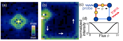
Figure 3: Microscopic simulation of the wavelength conversion scheme, Eq. (4), indicating its feasibility: Spatial distribution of light intensity upon local injection of a probe laser in the bulk (a) and at the edge (b), for a constant artificial magnetic field. Bulk transport (a) is governed by Landau levels and can be understood as a superposition of classical cyclotron orbits (yellow circles) for different momentum directions. (b) At the edges robust edge channels exist. (c) Optical Aharonov-Bohm effect in minimal symmetric setup: (d) The interference pattern (normalized probe laser transmission intensity) is shifted by the magnetic flux through the ring. [Parameters: 22x22 grid (a,b); $\delta=0.3\Omega_{0}$ (a,b), $\delta=0.1\Omega_{0}$ (d); $g=0.2\Omega_{0}$ (a,b), $g=0.01\Omega_{0}$ (d); $\kappa=0.01\Omega_{0}$; $\Gamma=\kappa/10$; $\Phi=2\pi/8$ (a,b); $J=0.13\Omega_{0}$ (a,b), $J=0.001\Omega_{0}$ (d), $\Delta_{p}=1.278\Omega_{0}$ (a), $\Delta_{p}=1.260\Omega_{0}$ (b), $\Delta_{p}=1.103\Omega_{0}$ (d)]

In addition to measuring the optical spectrum, it is also possible to look at photon transport in a spatially resolved manner, by injecting a probe laser locally and then imaging the photons leaving the sample. This provides another way to observe the effects of the artificial gauge field, which gives rise to distinct transport phenomena as depicted in Figure 3(a,b). For small magnetic fields, $|\phi|\ll 2\pi$, the dynamics can be understood in the continuum limit when probing the bulk: One recovers the standard Landau level picture for electrons in a constant magnetic field Hofstadter1976 ; LandauStatPhys2 , with effective mass $m^{*}=\hbar/2Ja^{2}$ and cyclotron frequency $\omega_{\text{cyc}}=2\phi J$, where $a$ is the lattice constant. In Figure 3 (a) the $n=1$ Landau level is selected via the probe’s detuning $\Delta_{p}$ with respect to the drive. The circles indicate the semi-classical cyclotron orbits with radius $R=a\sqrt{(2n+1)/\phi}$. In this semi-classical picture, the momentum of a photon injected locally at a site in the bulk is equally distributed over all directions, since the position is well-defined. Thus, the observed response resembles a superposition of semi-classical circular Lorentz trajectories with different initial velocity directions. A probe injected closer to the edge excites chiral integer Quantum Hall Effect edge states, see Fig. 3(b).

The Aharonov-Bohm effect Aharonov1959 is one of the most intriguing features of quantum mechanics. In an interferometer, electrons can acquire a phase difference determined by the magnetic flux enclosed by the interfering pathways, even though they never feel any force due to the magnetic field. Figure 3(c) depicts a setup that is based on the wavelength conversion scheme and realizes an optical analog of the Aharonov-Bohm effect: A local probe is transmitted via two pathways, leading to an interference pattern in the transmission. The pattern is shifted according to the flux through the ’ring’, see Fig. 3 (d), confirming the effect.

All the effects displayed in Fig. 3 have been simulated numerically for the wavelength conversion scheme, see Appendix C, but similar results hold for the modulated-link scheme.

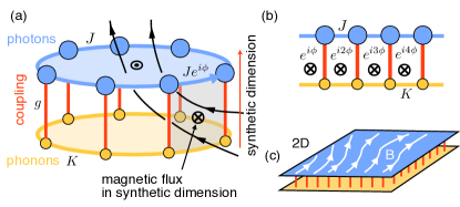
Figure 4: Optomechanical gauge fields within the concept of synthetic dimensions. (a) The optomechanical coupling, $g$, can be viewed as connecting sites along a synthetic dimension (photons vs. phonons). A phase for the photon hopping, engineered using the schemes from above, creates a flux in the optical plaquette (blue, top) and in the adjacent synthetic plaquette (gray). Hence, the magnetic field (black lines) in the full space is divergence-free. (b) Engineering exclusively the phases of $g$ allows to create magnetic fields/fluxes, but only perpendicular to the synthetic dimension. Shining a single tilted laser on a 1D chain yields a synthetic optomechanical ladder system with constant synthetic magnetic flux. (c) 2D array, with the field inside the (physical) plane generated by an arbitrary laser phase pattern.

So far we have analyzed schemes to engineer hopping phases for photons. We now ask about situations where the phonons are not only employed as auxiliary virtual excitations, but rather occur as real excitations, which can be interconverted with the photons. This means, in addition to the modes making up the lattices described above (in either of the two schemes), we now consider on-site vibrational modes $\hat{b}_{j}$ coupled optomechanically to the corresponding optical modes $\hat{a}_{j}$. Using the standard approach Aspelmeyer2013RMPArxiv , we arrive at a linearized optomechanical interaction of the form $-g\hat{a}_{j}^{\dagger}\hat{b}_{j}+\text{h.c.}$. Moreover, to be general (and generate nontrivial features connected to the gauge field structure), we will assume the neighboring phonon modes may also be coupled, as described by a tight-binding Hamiltonian of the form $-K\sum_{\langle ij\rangle}\hat{b}_{j}^{\dagger}\hat{b}_{i}+\text{h.c.}$.

When discussing the effects of gauge fields in such a setting, the system is best understood within the concept of ’synthetic’ dimensions Boada2012 ; Celi2014 . The optomechanical interaction can be viewed in terms of an extension of the 1D or 2D lattice into such an additional synthetic dimension. In our case, this dimension only has two discrete locations, corresponding to photons vs. phonons. In that picture, the optomechanical interaction, converting photons to phonons, corresponds to a simple hopping between sites along the additional direction. Figure 4 (a) sketches this for an optomechanical ring: photons and phonons represent two layers separated along the synthetic dimension. Applying any of our two previously discussed schemes, a photon hopping from site $i$ to $j$ will acquire a phase $\phi_{ij}=\int_{\vec{r}_{i}}^{\vec{r}_{j}}d\vec{r}\vec{A}$. The gauge field ${\bf A}$ must now be viewed as a vector field in this new 3d space, where one of the dimensions is synthetic. A finite hopping phase $\phi$ at one of the optical links creates a magnetic flux through the optical plaquette as desired, see Fig.  4 (a). However, and this is the important point, since the magnetic field ${\bf B}$ is divergence-free, the field must penetrate at least one additional plaquette, causing the opposite magnetic flux in the synthetic dimension (assuming $g\in\mathbb{R}$). In general, realizing that there is this kind of behaviour is crucial to avoid puzzles about seeming violations of gauge symmetry in situations with photon magnetic fields in optomechanical arrays. It is necessary to keep track of the full vector potential in the space that includes the synthetic dimension.

We now take a step back, getting rid of the previously discussed engineered schemes that required two lasers and some arrangement of ’link’ modes. Rather we will consider simple optomechanical arrays, i.e. lattices of optical and vibrational modes, with photon and phonon tunnel coupling between modes and with the optomechanical interaction. We ask: What is the effect of an arbitrary, spatially varying optical phase field in the driving laser that sets the strength of the optomechanical coupling? It turns out that the resulting spatially varying phase of the optomechanical coupling, $g_{j}=|g_{j}|e^{i\varphi_{j}}$, can be chosen to create arbitrary magnetic fields perpendicular to the synthetic dimension. A particularly simple example is a simple linear chain of optomechanical cells. Shining a tilted laser (i.e. with a phase gradient, $\varphi_{j}=j\cdot\delta\varphi$) onto such a 1D optomechanical array creates a constant magnetic flux through the plaquettes of the “optomechanical synthetic ladder” that can be drawn to understand the situation, cf. Figure 4 (b). The quantum mechanics of excitations tunneling between the two ’rails’ of the ladder (corresponding to photon-phonon conversion) is directly analogous to experiments on electron tunneling between parallel wires in a magnetic field Steinberg2008 . The magnetic field shifts the momenta of the tunneling particles, giving rise to resonance phenomena when the shifted dispersion curves $\omega(k)$ of the excitations match. Via phase front engineering one could create arbitrary synthetic magnetic fields also in 2D grids, see Figure 4(c). We note, though, that this method is constrained since it cannot create directly magnetic fluxes through optical or mechanical plaquettes, and in general only the schemes discussed above provide full flexibility. On the other hand, if either the photon or phonon modes are occupied only virtually, then effective fluxes can still be generated for the remaining real excitations, even with a single laser, and this works best for phonons (see Habraken2012 ; Peano2014 ).

We now discuss the most salient aspects of the experimental realization. Both the ’butterfly’ optical spectrum and spatially resolved transport can be probed using homodyne techniques, which are insensitive to noise. Real-space optical imaging is feasible, as the defects are a few micrometers apart. The optical phase pattern can be engineered using spatial light modulators. No time-dependent changes of the pattern are needed here, since the time-dependence is generated via the beat-note between the two laser beams.

For the modulated-link scheme, the mechanical oscillation amplitude $\beta$ used for the modulation should overwhelm any thermal fluctuations. In the example of Fig. 2, we assumed $g_{0}\beta=0.3\Omega_{0}$. At recently achieved parameters SafaviNaeini2014SnowCavity $g_{0}/2\pi=220\,\text{kHz}$ and $\Omega_{0}/2\pi=9\,\text{GHz}$ , this would imply $\beta\sim 10^{4}$, i.e. a phonon number of $10^{8}$ reached by driving, certainly larger than the thermal population. If we drive the mechanical vibration using a radiation pressure force oscillating at resonance (assuming the quoted $g_{0}$ also for the optical mode used in that driving), then we have $\beta=2g_{0}n_{c}/\Gamma$, where $n_{c}$ is the circulating photon number and $\Gamma$ the mechanical damping rate. Given a mechanical quality factor of $\Omega_{0}/\Gamma=2\cdot 10^{5}$, this requires $n_{c}\sim 10^{3}$ photons for Fig. 2, a realistic number. We note that thermal fluctuations of the mechanical amplitude give rise to a fractional deviation of $\sqrt{\bar{n}_{{\rm th}}}/\beta$ in $J_{{\rm eff}}$, with a slow drift on the time scale $\Gamma^{-1}$. At typical temperatures used in experiments, we have $\bar{n}_{{\rm th}}\sim 100-1000$, and so the fractional change is on the order of a percent, which will not noticeably impact transport.

In the alternative wavelength-conversion scheme, one should strive for a large photon-enhanced optomechanical coupling rate $g=g_{0}\alpha$. A general estimate implies we always need the photon number to be larger than $(\kappa/g_{0})^{2}$ in order to see the butterfly spectrum and the transport effects. This condition (compatible with Fig. 3) would require a circulating photon number of around $3\cdot 10^{5}$ for the parameters demonstrated in a recent successful wavelength conversion setup based on optomechanical crystals Hill2012WavelengthConversion . It is also important to estimate the unwanted influx of thermal excitations from the phonon subsystem into the photon subsystem, at least if the setup is to be applied in the quantum regime, for observing the transport of single photons in the presence of a magnetic field. In the wavelength-conversion scheme, there is a detuning $\delta\gg\kappa$ between the red sideband of the laser and the phonon mode, such that photon-phonon conversion is suppressed. Nevertheless, it still happens at a rate $\gamma\bar{n}$, where $\gamma=g^{2}/\delta$ is the “cooling rate” (for the detuned case applicable here) and $\bar{n}$ is the number of phonons in the mode. Fortunately, this phonon number is also reduced by the very same off-resonant cooling process. Balancing the inflow and outflow of excitations, we find that there will be a remaining unwanted photon occupation of $\bar{n}_{{\rm phot}}^{{\rm th}}=\bar{n}_{{\rm th}}\Gamma/\kappa$ due to the conversion of thermal phonons into photons, where $\bar{n}_{{\rm th}}$ is the bulk thermal phonon occupation. The factor $\Gamma/\kappa$ suppresses this number strongly, and it should be possible to reach the regime $\bar{n}_{{\rm phot}}^{{\rm th}}\ll 1$ in low-temperature setups.

Reducing fabrication-induced disorder will be crucial for any future applications of photonic crystals, including the one envisaged here (as well as other photonic magnetic field schemes). In first experimental attempts, the optical and mechanical disorder is on the percent level, which makes especially the fluctuations of the optical resonance frequencies significant. Nevertheless, strong reductions of the disorder will be possible by post-fabrication methods Zheng2011 ; Schmidt2009 ; Imamoglu2006 , such as local laser-induced oxidation. These are expected to reduce the fluctuations down to the level of $10^{-5}$ relative optical frequency fluctuations. This is enough to suppress the optical disorder to some fraction of the photon hopping rate $J_{{\rm eff}}\sim\Omega$, which will enable near-ideal photon transport (e.g. Anderson localization lengths would be at least hundreds of sites, larger than the typical arrays). Disorder in the mechanical frequencies can be reduced by similar techniques, but is much less problematic, due to the difference in absolute frequency scales between optics and mechanics.

Outlook - Optomechanical crystals represent an interesting system for the realization of artificial photonic magnetic fields due to their all-optical controllability. Moreover, their rich non-linear (quantum) dynamics Ludwig2013 could be explored in the presence of an artificial magnetic field. In general, the very flexible optical control could be used to create and explore novel features, e.g. varying the optomechanical coupling strength spatially and/or temporally, both adiabatically and with sudden quenches. Moreover, a second strong control laser could be used to create a spatially and temporarily varying optical on-site potential landscape.

Acknowledgements - This work was supported via an ERC Starting Grant OPTOMECH, the ITN cQOM, the DARPA program ORCHID, and via the Institute for Quantum Information and Matter, an NSF Physics Frontiers Center with support of the Gordon and Betty Moore Foundation.

Appendix A Derivation of the effective magnetic Hamiltonian for the modulated link scheme

Here, we derive the effective Hamiltonian $\hbar J_{{\rm eff}}e^{i\phi}\hat{a}{}_{B}^{\dagger}\hat{a}{}_{A}+\text{h.c.}$ that describes the tunneling of photons from site A to site B in the presence of an effective magnetic field created using the modulated link scheme. We start from the full time dependent Hamiltonian Eq. (3). Since this second-quantized Hamiltonian is particle conserving we can switch to a first-quantized picture in the standard way. The corresponding single-particle Hamiltonian $\hat{H}_{M}$ reads

$$\hat{H}_{M}=\hbar\begin{pmatrix}\omega_{A}&0&-J\\ 0&\omega_{B}&-J\\ -J&-J&\bar{\omega}_{I}+2g_{0}|\beta|\cos(\Omega t+\phi)\end{pmatrix}.$$

It acts on the photon wavefunction $|\psi\rangle\equiv(\psi_{A},\psi_{B},\psi_{I})$ where $\psi_{s}$ describes the probability amplitude that the photon is localized on site $s$, $s=A,B,I$. Since the Hamiltonian is time periodic, there is a complete set of quasi-periodic solutions of the Schrï¿œdinger equation, $|\psi_{j}(t+2\pi/\Omega)\rangle=\exp[-i2\pi\omega_{j}/\Omega]|\psi_{j}(t)\rangle$ where $2\pi/\Omega$ is the period and index $j$ spans the Hilbert space, $j=1,2,3$. In practice, one solves the eigenvalue problem $\varepsilon_{jm}\big{|}\phi_{jm}\rangle\rangle={\cal H}{}_{jm}\big{|}\phi_{jm}\rangle\rangle$ where ${\cal H}\equiv-i\hbar\partial_{t}+\hat{H}_{M}$ is the Floquet-Hamiltonian, $\varepsilon_{jm}=\hbar(\omega_{j}+m\Omega)$ are the quasienergies and $\big{|}\phi_{jm}\rangle\rangle=\exp[i(\omega_{j}+m\Omega)t]\big{|}\psi_{j}(t)\rangle$ are time-periodic states, the so-called Floquet eigenstates [$m\in\mathbb{Z}$] SAMBE1973 . Notice that the Floquet Hamiltonian can be regarded as an operator on the extended Hilbert space of the time periodic vectors equipped with the scalar product

$$\langle\langle\phi_{j}\big{|}\phi_{m}\rangle\rangle=\frac{1}{T}\int_{0}^{T}\langle\phi_{j}(t)|\phi_{m}(t)\rangle.$$ (5)

In this framework, we can use the standard quantum mechanical perturbation theory to derive an effective time independent single-particle Hamiltonian. We assume a resonant drive $\omega_{A}\approx\omega_{B}+\Omega$, and weak tunneling/driving, $J_{A,B}/|\omega_{A,B}-\bar{\omega}_{I}|$, $g_{0}\beta/\Omega\ll 1$. We identify resonant Floquet-levels with quasienergies $\hbar\omega_{A}$ and $\hbar(\omega_{B}+\Omega$) coupled via the third order virtual tunneling process through the interface site I shown in Figure 5. Up to leading order in perturbation theory, we can focus on the block of the Floquet Hamiltonian comprising the four unperturbed quasienergy levels that are involved in this process, cf. Figure 5,

$${\cal\hat{H}}=\hbar\begin{pmatrix}\omega_{A}&0&-J&0\\ 0&\omega_{B}+\Omega&0&-J\\ -J&0&\omega_{I}&g_{0}\beta\\ 0&-J&g_{0}\beta^{*}&\omega_{I}+\Omega\end{pmatrix}.$$

Application of a standard Schrieffer-Wolff transformation Schrieffer1966 ; Shavitt1980 ; Bravyi2011 , i.e. applying degenerate perturbation theory to third order, leads to the effective block diagonal Floquet Hamiltonian

$${\cal\hat{H}}_{{\rm eff}}=\hbar\begin{pmatrix}\tilde{\omega}_{A}&J_{{\rm eff}}e^{-i\phi}\\ J_{{\rm eff}}e^{i\phi}&\tilde{\omega}_{B}+\omega_{{\rm ex}}\end{pmatrix}.$$ (6)

where $\tilde{\omega}_{s}=\omega_{s}+J_{s}^{2}/(\omega_{s}-\bar{\omega}_{I})$ with $s=A,B$ and $J_{{\rm eff}}=g_{0}|\beta|J_{A}J_{B}/[(\omega_{A}-\bar{\omega}_{I})(\omega_{B}-\bar{\omega}_{I})]$. Finally, we turn back Hamiltonian 6 into its second-quantized form and switch to a frame rotating with frequency $\tilde{\omega}_{A}$ ($\tilde{\omega}_{B}$) on site A (B). For a resonant drive, $\tilde{\omega}_{A}=\tilde{\omega}_{B}+\Omega$, this yields the desired form of the second-quantized effective Hamiltonian, $J_{{\rm eff}}(e^{-i\phi}\hat{a}{}_{A}^{\dagger}\hat{a}{}_{B}+e^{i\phi}\hat{a}{}_{B}^{\dagger}\hat{a}{}_{A}).$

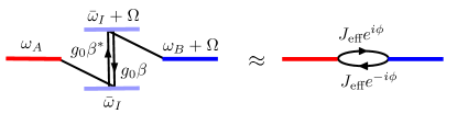
Figure 5: Floquet level scheme, i.e. quasienergy levels, describing the hopping transitions between sites $A$ and $B$ mediated by the virtual transition trough site $I$ accompanied by the exchange of a phonon.

Appendix B Transmission amplitudes and density of states for the modulated link scheme

Here, we calculate the LDOS for the modulated link scheme which is plotted in Figure 2. We use the full time dependent Hamiltonian Eq. (3) extended to the whole lattice (including also the sublattice formed by the link sites). Since we are dealing with a time periodic system where the energy is not a constant of motion, we have to appropriately generalize the definition of the LDOS. A natural generalization of the standard definition to time-periodic systems is the following,

$$\rho(\omega,\mathbf{j})=-2{\rm Im}G(\omega,0;\mathbf{j},\mathbf{j})$$

where $G(\omega,m;\mathbf{j},\mathbf{l})$ is the Floquet Green’s function

$$G=\frac{-i}{T}\int_{0}^{T}\!\!d\tau\int_{0}^{\infty}\!dte^{i(\omega+m\Omega)t+im\Omega\tau}\langle[\hat{a}_{\mathbf{j}}(t+\tau),\hat{a}_{\mathbf{l}}^{\dagger}(\tau)]\rangle.$$

The Floquet Green’s function describes the (linear) response of the array to a probe laser. More precisely, the light amplitude on site $\mathbf{j}$ in the presence of a probe drive on site $\mathbf{l}$ with frequency $\omega$ and amplitude $\alpha^{(in)}$ [described by the additional Hamiltonian term $H_{I}=i\hbar\sqrt{\kappa}\alpha^{(in)}(\hat{a}_{\mathbf{l}}^{\dagger}e^{-i\omega t}+h.c.)$] is

$$\langle\hat{a}_{\mathbf{j}}(t)\rangle=\sum_{m}e^{-i(\omega+m\Omega)t}i\sqrt{\kappa}\alpha^{(in)}G(\omega,m;\mathbf{j},\mathbf{l}).$$

This is essentially a generalization of the Kubo formula which applies to any time periodic Hamiltonian. Using the input-output relations, $\hat{a}_{\mathbf{j}}^{(out)}(t)=\hat{a}_{\mathbf{j}}^{(in)}(t)-\sqrt{\kappa}\hat{a}_{\mathbf{j}}$, we can also calculate the field outside the cavity,

$$\langle\hat{a}_{\mathbf{j}}^{(out)}(t)\rangle\equiv\sum_{m}e^{-i(\omega+m\Omega)t}t_{O}(\omega,m;\mathbf{j},\mathbf{l})\alpha^{(in)},$$

where

$$t_{O}(\omega,m;\mathbf{j},\mathbf{l})=\delta_{\mathbf{j\mathbf{l}}}\delta_{m0}-i\kappa G(\omega,m;\mathbf{j},\mathbf{l})$$

is the transmission amplitude of a photon from site $\mathbf{l}$ to site $\mathbf{j}$ if it has been up-converted $m$-times (or down-converted $|m|$-times for $m$ negative).

For a time-periodic system with a particle conserving Hamiltonian, the Floquet Green’s function can be easily expressed in terms of the first-quantized Floquet Hamiltonian ${\cal H}=-i\partial_{t}-H(t)$,

$$G(\omega,m;\mathbf{j},\mathbf{l})=\big{\langle}\big{\langle}\mathbf{j},m\big{|}\left(\omega-{\cal H}+i\kappa/2\right)^{-1}\big{|}\mathbf{l},0\big{\rangle}\big{\rangle}$$

Notice that the Floquet Hamiltonian and the Green’s function can be regarded as operators acting on the extended Hilbert space of the time-periodic photon states with the scalar product Eq. (5 ). As such they acts on the time periodic states $|\mathbf{j},m\rangle\rangle,$ where index $\mathbf{j}$ indicates the lattice site and $m$ the Fourier component. Thus, the density of states can be readily computed by diagonalizing the Floquet Green’s function. We find

$$\text{$\rho$}(\omega)=\sum_{k}\frac{\kappa}{(\omega-\omega_{k})^{2}+\kappa^{2}/4}\Big{|}\big{\langle}\big{\langle}\mathbf{j},0\big{|}\phi_{k}\big{\rangle}\big{\rangle}\Big{|}^{2}\,,$$

where $\hbar\omega_{k}$ are the quasienergies and $\big{|}\phi_{k}\rangle\rangle$ are the corresponding Floquet eigenstates obtained by numerically diagonalizing ${\cal H}$. Taking into account that the Floquet eigenfunctions $\big{|}\phi_{k}\rangle\rangle$ forms a complete orthonormal basis of the Hilbert space of the time-periodic states [with the scalar product Eq. (5 )], it immediately follows that the density of states is appropriately normalized,

$$\int_{-\infty}^{\infty}d\omega\rho(\omega)=2\pi.$$

Appendix C Transmission amplitudes for the frequency-conversion scheme

For the frequency-conversion scheme we start from the linearized Langevin equations for the full array including the mechanical links modes Aspelmeyer2013RMPArxiv ; Schmidt2014 ,

$$\dot{\hat{b}}_{\mathbf{k}} = i\hbar^{-1}[\hat{H},\hat{b}_{\mathbf{k}}]-\Gamma\hat{b}_{\mathbf{k}}/2+\sqrt{\Gamma}\hat{b}_{\mathbf{k}}^{({\rm in)}},$$

$$\dot{\hat{a}}_{\mathbf{j}} = i\hbar^{-1}[\hat{H},\hat{a}_{\mathbf{j}}]-\kappa\hat{a}_{\mathbf{j}}/2+\sqrt{\kappa}\hat{a}_{\mathbf{j}}^{({\rm in)}}.$$ (7)

The first line (second line) describes the sites hosting a mechanical (optical) mode. The Hamiltonian $\hat{H}$ is given by Eq. (4) extended to the full array and the noise forces have the usual commutation relations Aspelmeyer2013RMPArxiv . Notice that Eq. (7) is written in a frame where the optical modes on sublattice A and B are rotating with frequency $\omega_{L1}$ and $\omega_{L2}$, respectively. A probe laser on site $\mathbf{l}$ with frequency $\omega$ and amplitude $\alpha^{in}$ is described by the additional Hamiltonian term $H_{I}=i\hbar\sqrt{\kappa}\alpha^{(in)}(\hat{a}_{\mathbf{l}}^{\dagger}e^{-i\Delta_{p}t}-h.c.)$, where $\Delta_{p}=\omega-\omega_{Ls}$ ($s=1,2$ for $\mathbf{l}$ on sublattice A or B, respectively). The linear response of the light amplitude on site $\mathbf{j}$ to such probe laser is given by the Kubo formula

$$\langle\hat{a}_{\mathbf{j}}(t)\rangle = i\sqrt{\kappa}\alpha^{(in)}e^{-i\Delta_{p}t}G_{\hat{a}\hat{a}^{\dagger}}(\Delta_{p},\mathbf{j},\mathbf{l})$$ (8)

$$-i\sqrt{\kappa}\alpha^{(in)}e^{i\Delta_{p}t}G_{\hat{a}\hat{a}}(-\Delta_{p},\mathbf{j},\mathbf{l}),$$

with the Green’s functions

$$G_{\hat{a}\hat{a}^{\dagger}}(\omega,\mathbf{j},\mathbf{l}) =-i \int_{0}^{\infty}\!dte^{i\omega t}\langle[\hat{a}_{\mathbf{j}}(t),\hat{a}_{\mathbf{l}}^{\dagger}(0)]\rangle,$$

$$G_{\hat{a}\hat{a}}(\omega,\mathbf{j},\mathbf{l}) =-i \int_{0}^{\infty}\!dte^{i\omega t}\langle[\hat{a}_{\mathbf{j}}(t),\hat{a}_{\mathbf{l}}(0)]\rangle.$$

Notice that in Figure 3 and 4 of the main text we plot the resonant part of the response corresponding to the first line of Eq. (8). If $\mathbf{j}$ and $\mathbf{l}$ lie on different sublattices, the frequency of the probe signal is converted [to read off this frequency from Eq. (8), one has to keep in mind that the frame of reference is rotating at different frequencies on the two optical sublattices]. Finally, we note that the light transmitted outside of the sample $\left\langle\hat{a}_{\mathbf{j}}^{({\rm out})}\right\rangle=t(\omega,\mathbf{j},\mathbf{l})\left\langle\hat{a}_{\mathbf{l}}^{({\rm in})}\right\rangle$ can be readily computed using the input output relations WallsMilburn_QuantumOptics $\hat{a}_{\mathbf{j}}^{({\rm out})}=\hat{a}_{\mathbf{j}}^{({\rm in})}-\sqrt{\kappa}\hat{a}_{\mathbf{j}}$. From Eq. (8) we find the transmission amplitude

$$t_{O}(\omega,\mathbf{l},\mathbf{j})=\delta_{\mathbf{lj}}-i\kappa G_{\hat{a}\hat{a}^{\dagger}}(\omega,\mathbf{l},\mathbf{j}).$$ (9)

Since the transmission amplitudes of a probe laser beam are generally proportional to the corresponding light amplitudes inside the array (on all sites except for the one where the light is injected), the amplitude patterns shown in Figures 3 and 4 could be directly measured by a position resolved measurement of the light scattered by the array.

In order to calculate the transmission in Figures 3 and 4 we have calculated the Green’s function numerically. We note that for an array with $N\times N$ optical sites, there is a total of $N(2N-1)$ sites (including also the mechanical sites) and a total of $2N(2N-1)$ degrees of freedom. Thus, computing numerically the Green’s function amounts to inverting a $2N(2N-1)\times 2N(2N-1)$ matrix. In Figure 3 and 4 we have chosen $N=22$.

References

- (1) Markus Aspelmeyer, Tobias J. Kippenberg, and Florian Marquardt. Cavity optomechanics. Rev. Mod. Phys., 86:1391, 2014.
- (2) Amir H. Safavi-Naeini and Oskar Painter. Design of optomechanical cavities and waveguides on a simultaneous bandgap phononic-photonic crystal slab. Opt. Express, 18(14):14926–14943, 2010.
- (3) Matt Eichenfield, Jasper Chan, Ryan M. Camacho, Kerry J. Vahala, and Oskar Painter. Optomechanical crystals. Nature, 462(7269):78–82, 2009.
- (4) Amir H. Safavi-Naeini, Thiago P. Mayer Alegre, Martin Winger, and Oskar Painter. Optomechanics in an ultrahigh-q two-dimensional photonic crystal cavity. Appl. Phys. Lett., 97(18):181106, 2010.
- (5) E. Gavartin, R. Braive, I. Sagnes, O. Arcizet, A. Beveratos, T. J. Kippenberg, and I. Robert-Philip. Optomechanical coupling in a two-dimensional photonic crystal defect cavity. Phys. Rev. Lett., 106:203902, 2011.
- (6) Jasper Chan, T. P. Mayer Alegre, Amir H. Safavi-Naeini, Jeff T. Hill, Alex Krause, Simon Groblacher, Markus Aspelmeyer, and Oskar Painter. Laser cooling of a nanomechanical oscillator into its quantum ground state. Nature, 478(7367):89–92, 2011.
- (7) Amir H. Safavi-Naeini, Jeff T. Hill, Seán Meenehan, Jasper Chan, Simon Gröblacher, and Oskar Painter. Two-dimensional phononic-photonic band gap optomechanical crystal cavity. Phys. Rev. Lett., 112:153603, 2014.
- (8) Georg Heinrich, Max Ludwig, Jiang Qian, Björn Kubala, and Florian Marquardt. Collective dynamics in optomechanical arrays. Phys. Rev. Lett., 107:043603, 2011.
- (9) C. A. Holmes, C. P. Meaney, and G. J. Milburn. Synchronization of many nanomechanical resonators coupled via a common cavity field. Phys. Rev. E, 85:066203, 2012.
- (10) Max Ludwig and Florian Marquardt. Quantum many-body dynamics in optomechanical arrays. Phys. Rev. Lett., 111:073603, 2013.
- (11) M. Bhattacharya and P. Meystre. Multiple membrane cavity optomechanics. Phys. Rev. A, 78(4):041801, 2008.
- (12) André Xuereb, Claudiu Genes, and Aurélien Dantan. Strong coupling and long-range collective interactions in optomechanical arrays. Phys. Rev. Lett., 109:223601, 2012.
- (13) A. Tomadin, S. Diehl, M. D. Lukin, P. Rabl, and P. Zoller. Reservoir engineering and dynamical phase transitions in optomechanical arrays. Phys. Rev. A, 86:033821, 2012.
- (14) Michael Schmidt, Max Ludwig, and Florian Marquardt. Optomechanical circuits for nanomechanical continuous variable quantum state processing. New J. Phys., 14(12):125005, 2012.
- (15) Uzma Akram, William Munro, Kae Nemoto, and G. J. Milburn. Photon-phonon entanglement in coupled optomechanical arrays. Phys. Rev. A, 86:042306, 2012.
- (16) D E Chang, A H Safavi-Naeini, M Hafezi, and O Painter. Slowing and stopping light using an optomechanical crystal array. New J. Phys., 13(2):023003, 2011.
- (17) Wei Chen and Aashish A. Clerk. Photon propagation in a one-dimensional optomechanical lattice. Phys. Rev. A, 89:033854, 2014.
- (18) M. Schmidt, V. Peano, and F. Marquardt. Optomechanical dirac physics. New J. Phys., 17:023025, 2015.
- (19) Jens Koch, Andrew A. Houck, Karyn Le Hur, and S. M. Girvin. Time-reversal-symmetry breaking in circuit-qed-based photon lattices. Phys. Rev. A, 82:043811, Oct 2010.
- (20) Mohammad Hafezi, Eugene A. Demler, Mikhail D. Lukin, and Jacob M. Taylor. Robust optical delay lines with topological protection. Nature Physics, 7:907, August 2011.
- (21) R. O. Umucal ılar and I. Carusotto. Artificial gauge field for photons in coupled cavity arrays. Phys. Rev. A, 84:043804, Oct 2011.
- (22) Kejie Fang, Zongfu Yu, and Shanhui Fan. Realizing effective magnetic field for photons by controlling the phase of dynamic modulation. Nature Photonics, 6(11):782–787, 2012.
- (23) Mohammad Hafezi and Peter Rabl. Optomechanically induced non-reciprocity in microring resonators. Opt. Express, 20(7):7672–7684, Mar 2012.
- (24) M. Hafezi, S. Mittal, J. Fan, A. Migdall, and J. M. Taylor. Imaging topological edge states in silicon photonics. Nature Photonics, 7(12):1001–1005, 2013.
- (25) S. Mittal, J. Fan, S. Faez, A. Migdall, J. M. Taylor, and M. Hafezi. Topologically robust transport of photons in a synthetic gauge field. Phys. Rev. Lett., 113:087403, Aug 2014.
- (26) Mikael C. Rechtsman, Julia M. Zeuner, Yonatan Plotnik, Yaakov Lumer, Daniel Podolsky, Felix Dreisow, Stefan Nolte, Mordechai Segev, and Alexander Szameit. Photonic floquet topological insulators. Nature, 496(7444):196–200, 2013.
- (27) Alejandro Bermudez, Tobias Schaetz, and Diego Porras. Synthetic gauge fields for vibrational excitations of trapped ions. Phys. Rev. Lett., 107:150501, Oct 2011.
- (28) M. Aidelsburger, M. Atala, M. Lohse, J. T. Barreiro, B. Paredes, and I. Bloch. Realization of the hofstadter hamiltonian with ultracold atoms in optical lattices. Phys. Rev. Lett., 111:185301, Oct 2013.
- (29) Hirokazu Miyake, Georgios A. Siviloglou, Colin J. Kennedy, William Cody Burton, and Wolfgang Ketterle. Realizing the harper hamiltonian with laser-assisted tunneling in optical lattices. Phys. Rev. Lett., 111:185302, Oct 2013.
- (30) Lawrence D. Tzuang, Kejie Fang, Paulo Nussenzveig, Shanhui Fan, and Michal Lipson. Non-reciprocal phase shift induced by an effective magnetic flux for light. Nat Photon, 8(9):701–705, September 2014.
- (31) Georg Heinrich, J. G. E. Harris, and Florian Marquardt. Photon shuttle: Landau-zener-stückelberg dynamics in an optomechanical system. Phys. Rev. A, 81:011801, Jan 2010.
- (32) Jeff T. Hill, Amir H. Safavi-Naeini, Jasper Chan, and Oskar Painter. Coherent optical wavelength conversion via cavity-optomechanics. Nat. Commun., 3:1196, 2012.
- (33) Chunhua Dong, Victor Fiore, Mark C. Kuzyk, and Hailin Wang. Optomechanical dark mode. Science, 338(6114):1609–1613, 2012.
- (34) Douglas R. Hofstadter. Energy levels and wave functions of bloch electrons in rational and irrational magnetic fields. Phys. Rev. B, 14:2239–2249, Sep 1976.
- (35) L D Landau and E M Lifshitz. Statistical Physics, Part 2. Butterworth-Heinemann, 1980.
- (36) Y. Aharonov and D. Bohm. Significance of electromagnetic potentials in the quantum theory. Phys. Rev., 115:485–491, Aug 1959.
- (37) O. Boada, A. Celi, J. I. Latorre, and M. Lewenstein. Quantum simulation of an extra dimension. Phys. Rev. Lett., 108:133001, Mar 2012.
- (38) A. Celi, P. Massignan, J. Ruseckas, N. Goldman, I. B. Spielman, G. Juzeliunas, and M. Lewenstein. Synthetic gauge fields in synthetic dimensions. Phys. Rev. Lett., 112:043001, Jan 2014.
- (39) Hadar Steinberg, Gilad Barak, Amir Yacoby, Loren N. Pfeiffer, Ken W. West, Bertrand I. Halperin, and Karyn Le Hur. Charge fractionalization in quantum wires. Nat Phys, 4(2):116–119, February 2008.
- (40) S J M Habraken, K Stannigel, M D Lukin, P Zoller, and P Rabl. Continuous mode cooling and phonon routers for phononic quantum networks. New Journal of Physics, 14(11):115004, 2012.
- (41) V. Peano, C. Brendel, M. Schmidt, and F. Marquardt. Topological phases of sound and light. ArXiv, 1409.5375, 2014.
- (42) J. Zheng et al. Selective tuning of silicon photonic crystal cavities via laser-assisted local oxidation. Conference Paper CLEO AMA, 2011.
- (43) H. S. Lee et al. Local tuning of photonic crystal nanocavity modes by laser-assisted oxidation. Applied Physics Letters, 95:191109, 2009.
- (44) K. Hennessy, C. Högerle, E. Hu, A. Badolato, and A. Imamoglu. Tuning photonic nanocavities by atomic force microscope nano-oxidation. Applied Physics Letters, 89:041118, 2006.
- (45) Hideo Sambe. Steady states and quasienergies of a quantum-mechanical system in an oscillating field. Phys. Rev. A, 7:2203–2213, Jun 1973.
- (46) J. R. Schrieffer and P. A. Wolff. Relation between the anderson and kondo hamiltonians. Phys. Rev., 149:491–492, Sep 1966.
- (47) Isaiah Shavitt and Lynn T. Redmon. Quasidegenerate perturbation theories. a canonical van vleck formalism and its relationship to other approaches. The Journal of Chemical Physics, 73(11):5711–5717, 1980.
- (48) Sergey Bravyi, David P. DiVincenzo, and Daniel Loss. Schrieffer-wolff transformation for quantum many-body systems. Annals of Physics, 326(10):2793 – 2826, 2011.
- (49) D. F. Walls and G. J. Milburn. Quantum Optics. Springer, 2008.