Properties and examples of Faber–Walsh polynomials

Abstract

The Faber–Walsh polynomials are a direct generalization of the (classical) Faber polynomials from simply connected sets to sets with several simply connected components. In this paper we derive new properties of the Faber–Walsh polynomials, where we focus on results of interest in numerical linear algebra, and on the relation between the Faber–Walsh polynomials and the classical Faber and Chebyshev polynomials. Moreover, we present examples of Faber–Walsh polynomials for two real intervals as well as for some non-real sets consisting of several simply connected components.

Keywords Faber–Walsh polynomials, generalized Faber polynomials, multiply connected domains, lemniscatic domains, lemniscatic maps, conformal maps, asymptotic convergence factor

Mathematics Subject Classification (2010) 30C10; 30E10; 30C20

1 Introduction

The (classical) Faber polynomials associated with a simply connected compact set $\Omega\subset\mathbb{C}$ have found numerous applications in numerical approximation [11, 12] and in particular in numerical linear algebra [4, 7, 21, 30, 31, 43]. The main idea behind their construction, originally due to Faber [13], is to have a sequence of polynomials $F_{0},F_{1},F_{2},\dots$, so that each analytic function on $\Omega$ can be expanded in a convergent series of the form $\sum_{j=0}^{\infty}\gamma_{j}F_{j}(z)$, where the polynomials depend only on the set $\Omega$. The definition and practical computation of the Faber polynomials is based on the Riemann map from the exterior of $\Omega$ (in the extended complex plane) onto the exterior of the unit disk. The Faber polynomials therefore exist for simply connected sets only. For surveys of the theory of Faber polynomials we refer to [5, 44].

In 1956, Walsh found a direct generalization of the Riemann mapping theorem from simply connected domains to multiply connected domains, which now are mapped conformally onto a lemniscatic domain [45]; see Theorem 2.1 below for a complete statement. Further existence proofs of Walsh’s lemniscatic map were given by Grunsky [16, 17] and [18, Theorem 3.8.3], Jenkins [22] and Landau [25]. We recently studied lemniscatic maps in [41] and derived several explicit examples, which are among the first in the literature (see also the technical report [40]).

In a subsequent paper of 1958, Walsh used his lemniscatic map for obtaining a generalization of the Faber polynomials from simply connected sets to sets consisting of several simply connected components [46]; see Theorem 2.3 below for a complete statement. While the literature on Faber polynomials is quite extensive, the Faber–Walsh polynomials have rarely been studied in the literature. One notable exception is Suetin’s book [44], which contains a proper subsection on the Faber–Walsh polynomials as well as a few further references (see also the technical report [40]).

Clearly, the mathematical theory and practical applicability of the Faber–Walsh polynomials have not been fully explored yet. Our goal in this paper is to contribute to a better understanding. To this end we derive some new theoretical results on Faber–Walsh polynomials and give several analytic as well as numerically computed examples. In our theoretical study we focus on results that are of interest in constructive approximation and numerical linear algebra applications, and on the relation between Faber–Walsh polynomials and the classical Faber as well as Chebyshev polynomials. In our examples we consider sets consisting of two real intervals, as well as non-real sets consisting of several components. In particular, our numerical results demonstrate that the Faber–Walsh polynomials are computable for a wide range of sets via a numerical conformal mapping technique for multiply connected domains introduced in [32].

The paper is organized as follows. In Section 2 we give a summary of Walsh’s results, and recall the definition of Faber–Walsh polynomials. We then derive general properties of Faber–Walsh polynomials in Section 3. In Section 4 we consider Faber–Walsh polynomials for two real intervals and particularly study their relation to the classical Chebyshev polynomials. In Section 5 we show numerical examples of Faber–Walsh polynomials for two different nonreal sets.

2 The Faber–Walsh polynomials

We first discuss Walsh’s generalization of the Riemann mapping theorem. For a given integer $N\geq 1$, let $a_{1},\ldots,a_{N}\in\mathbb{C}$ be pairwise distinct and let the positive real numbers $m_{1},\ldots,m_{N}$ satisfy $\sum_{j=1}^{N}m_{j}=1$. Then for any $\mu>0$ the set

$$\mathcal{L}\mathrel{\mathop{:}}=\{w\in\widehat{\mathbb{C}}:|U(w)|>\mu\},\quad\text{where}\quad U(w)\mathrel{\mathop{:}}=\prod_{j=1}^{N}(w-a_{j})^{m_{j}},$$ (2.1)

is called a lemniscatic domain in the extended complex plane $\widehat{\mathbb{C}}=\mathbb{C}\cup\{\infty\}$. The following theorem of Walsh shows that lemniscatic domains are canonical domains for certain $N$-times connected domains (open and connected sets).

Theorem 2.1 ([45, Theorems 3 and 4]).

Let $E\mathrel{\mathop{:}}=\cup_{j=1}^{N}E_{j}$, where $E_{1},\ldots,E_{N}\subseteq\mathbb{C}$ are mutually exterior simply connected compact sets (none a single point), and let $\mathcal{K}\mathrel{\mathop{:}}=\widehat{\mathbb{C}}\backslash E$. Then there exists a unique lemniscatic domain $\mathcal{L}$ of the form (2.1) with $\mu>0$ equal to the logarithmic capacity of $E$, and a unique bijective conformal map

$$\Phi:\mathcal{K}\to\mathcal{L}\quad\text{with}\quad\Phi(z)=z+\mathcal{O}\left(\frac{1}{z}\right)\quad\text{for $z$ near infinity.}$$

We call the function $\Phi$ the lemniscatic map of $\mathcal{K}$ (or of $E$), and denote $\psi=\Phi^{-1}$.

For $N=1$ the set $E$ is simply connected and a lemniscatic domain is the exterior of a disk. Hence in this case Theorem 2.1 is equivalent with the Riemann mapping theorem. In [41] we studied the properties of lemniscatic maps and derived several analytic examples. In the subsequent paper [32], written jointly with Nasser, we presented a numerical method for computing lemniscatic maps. Both the analytic results from [41] and the numerical method from [32] will be used in Sections 4 and 5 below.

In [46] Walsh used Theorem 2.1 for proving the existence of a direct generalization of the (classical) Faber polynomials to sets $E$ with several components. The second major ingredient is the following. For the unit disk, the monomials $w^{k}$ are fundamental for Taylor and Laurent series of analytic functions, and the zeros of $w^{k}$ are at the center of the unit disk. For a lemniscatic domain $\mathcal{L}$, we need a generalization of $w^{k}$ to a polynomial with zeros at the foci $a_{1},\ldots,a_{N}$ of $\mathcal{L}$, and the multiplicity of each zero $a_{j}$ must correspond to its “importance” for $\mathcal{L}$, given by the exponent $m_{j}$.

Lemma 2.2 ([46, Lemma 2]).

Let $\mathcal{L}$ be a lemniscatic domain as in (2.1).

1. There exists a sequence $(\alpha_{j})_{j=1}^{\infty}$, chosen from the foci $a_{1},\ldots,a_{N}$, such that

   $$|N_{k,j}-km_{j}|\leq A\quad\text{for }j=1,2,\ldots,N,\quad k=1,2,\ldots,$$ (2.2)

   where $N_{k,j}$ denotes the number of times $a_{j}$ appears in the sequence $\alpha_{1},\ldots$, $\alpha_{k}$, and where $A>0$ is a constant.

2. Any such sequence has the following property: For any closed set $S\subseteq\widehat{\mathbb{C}}$ not containing any of the points $a_{1},\ldots,a_{N}$ there exist constants $A_{1},A_{2}>0$, such that

   $$A_{1}<\frac{|u_{k}(w)|}{|U(w)|^{k}}<A_{2}\quad\text{for }k=0,1,2,\ldots,\text{ and any }w\in S,$$ (2.3)

   where $u_{k}(w)\mathrel{\mathop{:}}=\prod_{j=1}^{k}(w-\alpha_{j})=\prod_{j=1}^{N}(w-a_{j})^{N_{k,j}}$.

For $N=1$ a lemniscatic domain is the exterior of a disk, and we have $\alpha_{j}=a_{1}$ for all $j\geq 1$ and $u_{k}(w)=(w-a_{1})^{k}$. For $N\geq 2$, the sequence $(\alpha_{j})_{j=1}^{\infty}$ is not unique, but it can be chosen constructively from $a_{1},\ldots,a_{N}$; see [46]. Note that a smaller constant $A$ in (2.2) implies better bounds in (2.3). For $N=2$ one possible choice is $\alpha_{j}=a_{1}$ if $\lfloor jm_{1}\rfloor>\lfloor(j-1)m_{1}\rfloor$, and $\alpha_{j}=a_{2}$ otherwise, where $\lfloor\cdot\rfloor$ denotes the integer part. We use this choice in our examples in Sections 4 and 5.1 below.

In the notation of Theorem 2.1, the Green’s functions with pole at infinity for $\mathcal{L}$ and $\mathcal{K}=\widehat{\mathbb{C}}\backslash E$ are

$$g_{\mathcal{L}}(w)=\log|U(w)|-\log(\mu)\quad\text{and}\quad g_{\mathcal{K}}(z)=g_{\mathcal{L}}(\Phi(z)),$$ (2.4)

respectively; see [41, 46]. For $\sigma>1$ we denote their level curves by

$$\begin{split}\Gamma_{\sigma}&=\{z\in\mathcal{K}:g_{\mathcal{K}}(z)=\log(\sigma)\},\\ \Lambda_{\sigma}&=\{w\in\mathcal{L}:g_{\mathcal{L}}(w)=\log(\sigma)\}=\{w\in\mathcal{L}:|U(w)|=\sigma\mu\}.\end{split}$$

Note that $\Phi(\Gamma_{\sigma})=\Lambda_{\sigma}$. Further, we denote by $\operatorname{int}$ and $\operatorname{ext}$ the interior and exterior of a closed curve (or union of closed curves), respectively. In particular, we have

$$\operatorname{int}(\Lambda_{\sigma})=\{w\in\widehat{\mathbb{C}}:|U(w)|<\sigma\mu\},\quad\operatorname{ext}(\Lambda_{\sigma})=\{w\in\widehat{\mathbb{C}}:|U(w)|>\sigma\mu\}.$$

We can now state Walsh’s main result from [46].

Theorem 2.3 ([46, Theorem 3]).

Let $E$, $\mathcal{L}$ and $\psi=\Phi^{-1}$ be as in Theorem 2.1. Let $(\alpha_{j})_{j=1}^{\infty}$ and the corresponding polynomials $u_{k}(w)$, $k=0,1,\ldots$, be as in Lemma 2.2. Then the following hold:

1. For $z\in\Gamma_{\sigma}$ and $w\in\operatorname{ext}(\Lambda_{\sigma})$ we have

   $$\frac{\psi^{\prime}(w)}{\psi(w)-z}=\sum_{k=0}^{\infty}\frac{b_{k}(z)}{u_{k+1}(w)},$$ (2.5)

   where

   $$b_{k}(z)=\frac{1}{2\pi i}\int_{\Lambda_{\lambda}}u_{k}(\tau)\frac{\psi^{\prime}(\tau)}{\psi(\tau)-z}\,d\tau=\frac{1}{2\pi i}\int_{\Gamma_{\lambda}}\frac{u_{k}(\Phi(\zeta))}{\zeta-z}\,d\zeta$$ (2.6)

   for any $\lambda>\sigma$. The function $b_{k}$ is a monic polynomial of degree $k$, which is called the $k$th Faber–Walsh polynomial for $E$ and $(\alpha_{j})_{j=1}^{\infty}$.

2. Let $f$ be analytic on $E$, and let $\rho>1$ be the largest number such that $f$ is analytic and single-valued in $\operatorname{int}(\Gamma_{\rho})$. Then $f$ has a unique representation as a Faber–Walsh series

   $$f(z)=\sum_{k=0}^{\infty}a_{k}b_{k}(z),\quad a_{k}=\frac{1}{2\pi i}\int_{\Lambda_{\lambda}}\frac{f(\psi(\tau))}{u_{k+1}(\tau)}\,d\tau,\quad 1<\lambda<\rho,$$

   which converges absolutely in $\operatorname{int}(\Gamma_{\rho})$ and maximally on $E$, i.e.,

   $$\limsup_{n\to\infty}\|f-\sum_{k=0}^{n}a_{k}b_{k}\|_{E}^{\frac{1}{n}}=\frac{1}{\rho},$$

   where $\|\cdot\|_{E}$ denotes the maximum norm on $E$.

Note that the assertions about the Faber–Walsh polynomials hold for any admissible sequence $(\alpha_{j})_{j=1}^{\infty}$ as in Lemma 2.2. In this article, if we do not explicitly mention the sequence, the corresponding results hold for any such sequence.

For $N=1$ the Faber–Walsh polynomials reduce to the monic Faber polynomials for the (simply connected) set $E$ as considered in [11, 29, 42].

For an entire function $f$ we have $\rho=\infty$ and hence $\operatorname{int}(\Gamma_{\rho})=\mathbb{C}$ in part 2. of the theorem.

In our proof of Proposition 3.6 below we will use that for each given $\sigma>1$ there exists positive constants $C_{1},C_{2}$ independent of $k$ such that

$$0<C_{1}|u_{k}(\Phi(z))|\leq|b_{k}(z)|\leq C_{2}|u_{k}(\Phi(z))|\quad\text{for }z\in\Gamma_{\sigma}.$$ (2.7)

Here the upper bound on $|b_{k}(z)|$ holds for all $k$ and the lower bound holds only for sufficiently large $k$; see [44, p. 253].

In (2.5)–(2.6) the Faber–Walsh polynomials are defined as the (polynomial) coefficients in the expansion of the function $\psi^{\prime}(w)/(\psi(w)-z)$. Similar to the (classical) Faber polynomials, the Faber–Walsh polynomials can also be defined using the coefficients of the Laurent series of the conformal map $\psi$ in a neighborhood of infinity. Using this approach one can derive a recursive formula for computing the Faber–Walsh polynomials. In the following result we state the recursion that we have used in our numerical computations that are described in Section 4.1. A variant of this recursion was first published in the technical report [40].

Proposition 2.4.

In the notation of Theorem 2.3, the Laurent series at infinity of the conformal map $\psi=\Phi^{-1}$ has the form

$$\psi(w)=w+\sum_{k=1}^{\infty}\frac{c_{k}}{w^{k}}.$$

Then the Faber–Walsh polynomials are recursively given by

$$\begin{split}b_{0}(z)&=1\\ b_{k}(z)&=(z-\alpha_{k})b_{k-1}(z)+\beta_{k-1,1}(z),\quad k\geq 1,\end{split}$$

where the $\beta_{k,\ell}(z)$ are polynomials given by $\beta_{0,1}(z)=0$ and

$$\begin{split}\beta_{1,\ell}(z)&=\alpha_{1}(\ell-1)c_{\ell-1}-(\ell+1)c_{\ell},\quad\ell\geq 1,\\ \beta_{k,\ell}(z)&=-c_{\ell}b_{k-1}(z)-\alpha_{k}\beta_{k-1,\ell}(z)+\beta_{k-1,\ell+1}(z),\quad k\geq 2,\quad\ell\geq 1,\end{split}$$

with $c_{0}=0$.

3 On the theory of Faber–Walsh polynomials

In this section we derive several new results about Faber–Walsh polynomials. We begin with an alternative representation, and then relate Faber polynomials for a simply connected set $\Omega$ to the Faber–Walsh polynomials for a polynomial pre-image of $\Omega$. Finally, we will show that the normalized Faber–Walsh polynomials are asymptotically optimal.

Our first result is an easy consequence of Theorem 2.3.

Corollary 3.1.

In the notation of Theorem 2.3, the $k$th Faber–Walsh polynomial $b_{k}(z)$ is the polynomial part of the Laurent series at infinity of $u_{k}(\Phi(z))$.

Proof.

By Theorem 2.1, the Laurent series at infinity of the lemniscatic map $\Phi$ has the form $\Phi(\zeta)=\zeta+\sum_{j=1}^{\infty}\frac{d_{j}}{\zeta^{j}}$, and thus

$$u_{k}(\Phi(\zeta))=\prod_{j=1}^{k}(\Phi(\zeta)-\alpha_{j})=p_{k}(\zeta)+\sum_{j=1}^{\infty}\frac{\widetilde{d}_{j}}{\zeta^{j}},$$

where $p_{k}$ is a monic polynomial of degree $k$. For $z\in\mathbb{C}$ and $\lambda>1$ sufficiently large, (2.6) yields

$$\begin{split}b_{k}(z)&=\frac{1}{2\pi i}\int_{\Gamma_{\lambda}}\frac{u_{k}(\Phi(\zeta))}{\zeta-z}\,d\zeta=\frac{1}{2\pi i}\int_{\Gamma_{\lambda}}\frac{p_{k}(\zeta)}{\zeta-z}\,d\zeta+\frac{1}{2\pi i}\int_{\Gamma_{\lambda}}\sum_{j=1}^{\infty}\frac{\widetilde{d}_{j}}{\zeta^{j}}\frac{1}{\zeta-z}\,d\zeta\\ &=p_{k}(z).\end{split}$$

The second integral vanishes by virtue of Cauchy’s integral formula for domains with infinity as interior point; see, e.g., [28, Problem 14.14]. ∎

Note that in the case $N=1$ this result reduces to the classical fact that the $k$th Faber polynomial $F_{k}(z)$ is the polynomial part of the Laurent series at infinity of $(\Phi(z))^{k}$.

We will now consider sets $E$ that are polynomial pre-images of simply connected sets $\Omega$. We first recall the following result from [41] about the corresponding lemniscatic maps, where $\Omega=\Omega^{*}=\{\overline{z}:z\in\Omega\}$ means that $\Omega$ is symmetric with respect to the real line.

Theorem 3.2 ([41, Theorem 3.1]).

Let $\Omega=\Omega^{*}\subseteq\mathbb{C}$ be a simply connected compact set (not a single point) with exterior Riemann mapping

$$\widetilde{\Phi}:\widehat{\mathbb{C}}\backslash\Omega\to\{w\in\widehat{\mathbb{C}}:|w|>1\},\quad\widetilde{\Phi}(\infty)=\infty,\quad\widetilde{\Phi}^{\prime}(\infty)>0.$$

Let $P(z)=\alpha z^{n}+\alpha_{0}$ with $\alpha>0$, $n\geq 2$, and $\alpha_{0}<\min(\Omega\cap\mathbb{R})$. Then $E\mathrel{\mathop{:}}=P^{-1}(\Omega)$ is the disjoint union of $n$ simply connected compact sets, and

$$\Phi:\widehat{\mathbb{C}}\backslash E\to\mathcal{L}=\{w\in\widehat{\mathbb{C}}:|U(w)|>\mu\},\quad\Phi(z)=z\Big{(}\frac{\mu^{n}}{z^{n}}[\widetilde{\Phi}(P(z))-\widetilde{\Phi}(P(0))]\Big{)}^{\frac{1}{n}},$$

is the lemniscatic map of $E$, where we take the principal branch of the $n$th root, and where

$$\mu\mathrel{\mathop{:}}=\Big{(}\frac{1}{\alpha\widetilde{\Phi}^{\prime}(\infty)}\Big{)}^{\frac{1}{n}}>0,\quad\text{and}\quad U(w)\mathrel{\mathop{:}}=(w^{n}+\mu^{n}\widetilde{\Phi}(P(0)))^{\frac{1}{n}}.$$

Note that we consider the Riemann map onto the exterior of the unit disk, so that $\widetilde{\Phi}^{\prime}(\infty)$ is positive, but is not necessarily $1$. Therefore, the Faber polynomials $F_{k}$ associated with this map have the leading coefficients $(\widetilde{\Phi}^{\prime}(\infty))^{k}$, and will in general not be monic.

We then obtain the following “transplantation result” for Faber–Walsh polynomials, which is an analogue of a similar result for Chebyshev polynomials shown in [15, 23]. For related results on polynomial pre-images see also [33, 35].

Theorem 3.3.

In the notation of Theorem 3.2, denote the $n\geq 2$ distinct roots of the polynomial $(U(w))^{n}$ by $a_{1},\ldots,a_{n}$. Then, the $(kn)$th Faber–Walsh polynomial for $E$ and $(\alpha_{j})_{j=1}^{\infty}=(a_{1},a_{2},\ldots,a_{n},a_{1},a_{2},\ldots,a_{n},\ldots)$ satisfies

$$b_{kn}(z)=\frac{1}{(\alpha\widetilde{\Phi}^{\prime}(\infty))^{k}}F_{k}(P(z)),$$ (3.1)

for all $k\geq 0$, where $F_{k}$ is the $k$th Faber polynomial for $\Omega$.

Proof.

Theorem 3.2 implies that

$$\prod_{j=1}^{n}(\Phi(z)-a_{j})=(U(\Phi(z)))^{n}=\mu^{n}\widetilde{\Phi}(P(z))=\frac{1}{\alpha\widetilde{\Phi}^{\prime}(\infty)}\widetilde{\Phi}(P(z)).$$

Then, for $k\geq 0$, we find

$$u_{kn}(\Phi(z))=\prod_{j=1}^{n}(\Phi(z)-a_{j})^{k}=\frac{1}{(\alpha\widetilde{\Phi}^{\prime}(\infty))^{k}}(\widetilde{\Phi}(P(z)))^{k}.$$

Considering on both sides the polynomial part of the Laurent series at infinity, we find (3.1); see Corollary 3.1 for the Faber–Walsh polynomials, and, for instance, [44, p. 33] for the Faber polynomials. ∎

In Theorem 3.3 other choices of the sequence $(\alpha_{j})_{j=1}^{\infty}$ are possible: If $(\alpha_{j})_{j=1}^{\infty}$ satisfies $u_{kn}(w)=\prod_{j=1}^{n}(w-a_{j})^{k}$ for some $k$, then (3.1) holds for this $k$.

For a polynomial of degree $1$ the situation is different from the one in Theorem 3.3, since the polynomial then is a linear transformation and thus preserves the number of components of a set. In this case we obtain the following stronger result.

Proposition 3.4.

Let the notation be as in Theorem 2.3, and let $P(z)=\alpha z+\beta$ with $\alpha,\beta\in\mathbb{C}$ and $\alpha\neq 0$. Then the Faber–Walsh polynomials $\widetilde{b}_{k}$ for $P(E)$ and $(P(\alpha_{j}))_{j=1}^{\infty}$ satisfy $b_{k}(z)=\frac{1}{\alpha^{k}}\widetilde{b}_{k}(P(z))$ for all $k\geq 0$.

Proof.

Let $\Phi:\widehat{\mathbb{C}}\backslash E\to\mathcal{L}$ be the lemniscatic map of $E$. Then $P(\mathcal{L})$ is a lemniscatic domain and $\widetilde{\Phi}\mathrel{\mathop{:}}=P\circ\Phi\circ P^{-1}$ is the lemniscatic map of $P(E)$; see [41, Lemma 2.3]. In particular, the polynomials $u_{k}(w)=\prod_{j=1}^{k}(w-\alpha_{j})$ for $\mathcal{L}$ and $\widetilde{u}_{k}(\widetilde{w})=\prod_{j=1}^{k}(\widetilde{w}-P(\alpha_{j}))$ for $P(\mathcal{L})$ satisfy

$$\widetilde{u}_{k}(\widetilde{\Phi}(P(z)))=\widetilde{u}_{k}(P(\Phi(z)))=\prod_{j=1}^{k}(P(\Phi(z))-P(\alpha_{j}))=\alpha^{k}u_{k}(\Phi(z)).$$

Corollary 3.1 implies that $\widetilde{b}_{k}(P(z))=\alpha^{k}b_{k}(z)$. ∎

We now show that Faber–Walsh polynomials are asymptotically optimal in the sense of the following definition introduced by Eiermann, Niethammer and Varga [9, 10] in the context of semi-iterative methods for solving linear algebraic systems.

Definition 3.5.

For a compact set $E\subseteq\mathbb{C}$ and $z_{0}\in\mathbb{C}$ the number

$$R_{z_{0}}(E)\mathrel{\mathop{:}}=\limsup_{k\to\infty}\Big{(}\min_{p\in\mathcal{P}_{k}(z_{0})}\|p\|_{E}\Big{)}^{1/k}$$

is called the asymptotic convergence factor for polynomials from $\mathcal{P}_{k}(z_{0})\mathrel{\mathop{:}}=\{1+\sum_{j=1}^{k}a_{j}(z-z_{0})^{j}:a_{1},\ldots,a_{k}\in\mathbb{C}\}$ on $E$. A sequence of polynomials $p_{k}\in\mathcal{P}_{k}(z_{0})$, $k=0,1,\ldots$, is called asymptotically optimal on $E$ and with respect to $z_{0}$, if

$$\lim_{k\to\infty}\|p_{k}\|_{E}^{1/k}=R_{z_{0}}(E).$$

For any compact set $E$ and $z_{0}\in\mathbb{C}$ we have $R_{z_{0}}(E)\leq 1$, and $R_{z_{0}}(E)=1$ if $z_{0}\in E$. More precisely, one can show that $R_{z_{0}}(E)<1$ if and only if $z_{0}$ is in the unbounded component of $\widehat{\mathbb{C}}\backslash E$.

Let $E$ be a compact set as in Theorem 2.1 and let $g_{\mathcal{K}}$ be the Green’s function with pole at infinity for $\mathcal{K}=\widehat{\mathbb{C}}\backslash E$, which is connected. Then the Bernstein–Walsh Lemma (see, e.g., [36, Theorem 5.5.7 (a)] or [47, Section 4.6]) says that any polynomial $p$ of degree $k\geq 1$ satisfies

$$\left(\frac{|p(z_{0})|}{\|p\|_{E}}\right)^{1/k}\leq\exp(g_{\mathcal{K}}(z_{0}))\quad\mbox{for all $z_{0}\in\mathbb{C}\setminus E$.}$$

Together with [36, Theorem 5.5.7 (b)] this yields

$$R_{z_{0}}(E)=\exp(-g_{\mathcal{K}}(z_{0}))=\frac{\mu}{|U(\Phi(z_{0}))|}$$ (3.2)

(the second equality follows from (2.4)) and the lower bound

$$\|p\|_{E}\geq R_{z_{0}}(E)^{k}\quad\mbox{for any }p\in\mathcal{P}_{k}(z_{0}).$$ (3.3)

Both (3.2) and (3.3) have been shown for $z_{0}=1\notin E$ in [8], and the proof given there can be easily extended to all $z_{0}\in\mathbb{C}\backslash E$.

Note that (3.2) is a formula for the asymptotic convergence factor for any complex set $E$ as in Theorem 2.1 and any $z_{0}\in\mathbb{C}\backslash E$. (For all other $z_{0}$ we have $R_{z_{0}}(E)=1$ as mentioned above.) Using (3.2) together with the numerical method from [32] for computing lemniscatic maps gives a numerical method for computing the asymptotic convergence factor for a large class of compact sets and arbitrary constraint points. This method is used in our numerical examples in Sections 4 and 5 below.

The inequality (3.3) belongs to the family of Bernstein–Walsh type inequalities. They are widely used in the literature in particular in the context of iterative methods for solving linear algebraic systems; see, e.g., [6, 8, 39] and the references cited therein. For $E$ consisting of a finite number of real intervals an improved lower bound for $\|p\|_{E}$, $p\in\mathcal{P}_{k}(0)$, has been derived in [39].

Proposition 3.6.

In the notation of Theorem 2.3, let $z_{0}\in\mathbb{C}\backslash E$ and let $\sigma_{0}>1$ be such that $z_{0}\in\Gamma_{\sigma_{0}}$. Then

$$R_{z_{0}}(E)=\frac{1}{\sigma_{0}}\quad\text{ and }\quad R_{z_{0}}(\overline{\operatorname{int}(\Gamma_{\sigma})})=\frac{\sigma}{\sigma_{0}}\quad\text{for }1<\sigma\leq\sigma_{0},$$

and the Faber–Walsh polynomials for $E$ satisfy

$$\lim_{k\to\infty}\Big{(}\frac{\|b_{k}\|_{E}}{|b_{k}(z_{0})|}\Big{)}^{1/k} =\frac{1}{\sigma_{0}}=R_{z_{0}}(E),$$ (3.4)

$$\lim_{k\to\infty}\Big{(}\frac{\|b_{k}\|_{\Gamma_{\sigma}}}{|b_{k}(z_{0})|}\Big{)}^{1/k} =\frac{\sigma}{\sigma_{0}}\quad\text{for any }\sigma>1.$$ (3.5)

Hence the normalized Faber–Walsh polynomials $b_{k}(z)/b_{k}(z_{0})\in\mathcal{P}_{k}(z_{0})$ are asymptotically optimal on $E$, and on $\overline{\operatorname{int}(\Gamma_{\sigma})}$ whenever $1<\sigma\leq\sigma_{0}$.

Proof.

The Green’s function with pole at infinity for $\mathcal{K}=\widehat{\mathbb{C}}\backslash E$ is $g_{\mathcal{K}}$ as in (2.4). By the definition of $\sigma_{0}$, we have $g_{\mathcal{K}}(z_{0})=\log(\sigma_{0})$, so that $R_{z_{0}}(E)=\frac{1}{\sigma_{0}}$ by (3.2). The Green’s function with pole at infinity for $\operatorname{ext}(\Gamma_{\sigma})$ is $g_{\mathcal{K}}(z)-\log(\sigma)$. Hence, for $1<\sigma\leq\sigma_{0}$, $R_{z_{0}}(\overline{\operatorname{int}(\Gamma_{\sigma})})=\tfrac{\sigma}{\sigma_{0}}$ by (3.2).

Let $\sigma>1$. By (2.7) there exists constants $C_{1},C_{2}>0$ such that for sufficiently large $k$ we have

$$C_{1}|u_{k}(\Phi(z))|<|b_{k}(z)|<C_{2}|u_{k}(\Phi(z))|,\quad z\in\Gamma_{\sigma}.$$

Apply Lemma 2.2 to bound $|u_{k}(\Phi(z))|$: There exist $A_{1},A_{2}>0$ such that (2.3) holds for $w\in\Phi(\Gamma_{\sigma})=\Lambda_{\sigma}=\{w:|U(w)|=\sigma\mu\}$. We thus have

$$C_{1}A_{1}(\sigma\mu)^{k}<|b_{k}(z)|<C_{2}A_{2}(\sigma\mu)^{k},\quad z\in\Gamma_{\sigma}.$$ (3.6)

We then have $b_{k}(z)\neq 0$ for $z\in\Gamma_{\sigma}$ and, in particular, $b_{k}(z_{0})\neq 0$ for sufficiently large $k$. Now (3.6) implies $\lim_{k\to\infty}|b_{k}(z)|^{1/k}=\sigma\mu$ for any $z\in\Gamma_{\sigma}$, and, in particular,

$$\lim_{k\to\infty}|b_{k}(z_{0})|^{1/k}=\sigma_{0}\mu.$$ (3.7)

Moreover $\lim_{k\to\infty}\|b_{k}\|_{\Gamma_{\sigma}}^{1/k}=\sigma\mu$, since (3.6) holds uniformly for $z\in\Gamma_{\sigma}$. This establishes (3.5).

It remains to show (3.4). We have $\|b_{k}\|_{E}\geq\mu^{k}$, since the Faber–Walsh polynomials $b_{k}$ are monic of degree $k$ and $\mu$ is the capacity of $E$; see [36, Theorem 5.5.4]. Hence

$$\mu^{k}\leq\|b_{k}\|_{E}\leq\|b_{k}\|_{\Gamma_{\sigma}}\leq C_{2}A_{2}(\sigma\mu)^{k},$$

where $\sigma>1$ is arbitrary; see (3.6). This shows that

$$\mu\leq\liminf_{k\to\infty}\|b_{k}\|_{E}^{1/k}\leq\limsup_{k\to\infty}\|b_{k}\|_{E}^{1/k}\leq\sigma\mu,$$

and $\lim_{k\to\infty}\|b_{k}\|_{E}^{1/k}=\mu$, since $\sigma>1$ was arbitrary. Together with (3.7) we obtain (3.4). ∎

4 Faber–Walsh polynomials on two real intervals

In this section we consider Faber–Walsh polynomials on sets consisting of two real intervals.

Polynomial approximation problems on such sets have been studied in numerous publications, dating back (at least) to the classical works of Achieser [2, 3], who derived analytic formulae for the Chebyshev polynomials and the Green’s function in terms of Jacobi’s elliptic and theta functions. For a modern treatment of this area with many references up to 1996 we refer to Fischer’s book [14]. It also contains an analytic formula for the asymptotic convergence factor for two intervals and real $z_{0}$ in terms of Jacobi’s elliptic and theta functions (through its characterization with the Green’s function), as well as a MATLAB code for its numerical computation [14, p. 130]. More recently, Peherstorfer and Schiefermayr studied Chebyshev polynomials on several real intervals in [34], and Schiefermayr derived bounds for the asymptotic convergence factor for two intervals in terms of elementary functions [38]. Related approximation problems have been studied in [20, 37, 39].

In this section we show how the Faber–Walsh polynomials fit into this widely studied area. We first consider the case of two intervals of the same length. Here the lemniscatic map is known explicitly, so that the Faber–Walsh polynomials can be explicitly computed and related to the classical Faber and Chebyshev polynomials. We then consider the general case of two arbitrary intervals, where we compute the lemniscatic map and the Faber–Walsh polynomials numerically.

4.1 Two intervals of the same length

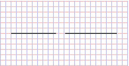
We consider the sets consisting of two real intervals of the same length which are symmetric with respect to the origin, i.e.,

$$E=[-D,-C]\cup[C,D]\quad\text{with }0<C<D.$$ (4.1)

The lemniscatic map of such a set is known analytically from [41].

Proposition 4.1.

Let $E$ be as in (4.1). Then

$$w=\Phi(z)=z\left(\frac{1}{2}+\frac{DC}{2}\frac{1}{z^{2}}\pm\frac{1}{2z^{2}}\sqrt{(z^{2}-C^{2})(z^{2}-D^{2})}\right)^{1/2}$$

is the lemniscatic map of $E$, and the corresponding lemniscatic domain is

$$\mathcal{L}=\left\{w\in\widehat{\mathbb{C}}:\left|w-\tfrac{D+C}{2}\right|^{1/2}\left|w+\tfrac{D+C}{2}\right|^{1/2}>\tfrac{\sqrt{D^{2}-C^{2}}}{2}\right\}.$$ (4.2)

Moreover, the inverse of $\Phi$ is given by

$$z=\psi(w)=w\sqrt{1+\left(\frac{D-C}{2}\right)^{2}\frac{1}{w^{2}-(\frac{D+C}{2})^{2}}},$$

where we take the principal branch of the square root. Its Laurent series at infinity is

$$\psi(w)=w+\sum_{k=0}^{\infty}\frac{c_{2k+1}}{w^{2k+1}},$$ (4.3)

where the coefficients are given by $c_{2k}=0$, $k\geq 0$, and

$$c_{2k+1}=\frac{1}{2}\left(\frac{D-C}{2}\right)^{2}\left(\frac{D+C}{2}\right)^{2k}-\frac{1}{2}\sum_{j=1}^{k}c_{2j-1}c_{2(k-j)+1},\quad k\geq 0.$$ (4.4)

In particular, $c_{1}=\frac{1}{2}\left(\frac{D-C}{2}\right)^{2}$.

Proof.

The construction of $\Phi$ and $\psi$ is given in [41, Corollary 3.3]. It thus remains to show the series expansion (4.3)–(4.4).

The function $w\mapsto\sqrt{1+\left(\frac{D-C}{2}\right)^{2}\tfrac{1}{w^{2}-(\frac{D+C}{2})^{2}}}$ is analytic and even in $\mathcal{L}$, and thus has a uniformly convergent Laurent series at infinity of the form

$$\sqrt{1+\left(\frac{D-C}{2}\right)^{2}\frac{1}{w^{2}-(\frac{D+C}{2})^{2}}}=\sum_{k=0}^{\infty}\frac{d_{k}}{w^{2k}}.$$ (4.5)

Setting $w=\infty$ shows $d_{0}=1$. Squaring (4.5) and expanding the left-hand side into a Laurent series yields

$$1+\sum_{k=1}^{\infty}\left(\frac{D-C}{2}\right)^{2}\left(\frac{D+C}{2}\right)^{2(k-1)}\frac{1}{w^{2k}}=\left(\sum_{k=0}^{\infty}\frac{d_{k}}{w^{2k}}\right)^{2}=\sum_{k=0}^{\infty}\sum_{j=0}^{k}d_{j}d_{k-j}\frac{1}{w^{2k}}.$$

For $k\geq 1$ we see that

$$\left(\frac{D-C}{2}\right)^{2}\left(\frac{D+C}{2}\right)^{2(k-1)}=\sum_{j=0}^{k}d_{j}d_{k-j}=2d_{0}d_{k}+\sum_{j=1}^{k-1}d_{j}d_{k-j},$$

and thus

$$d_{k}=\frac{1}{2}\left(\frac{D-C}{2}\right)^{2}\left(\frac{D+C}{2}\right)^{2(k-1)}-\frac{1}{2}\sum_{j=1}^{k-1}d_{j}d_{k-j},\quad k\geq 1.$$

Since $\psi(w)=w+\sum_{k=0}^{\infty}\frac{d_{k+1}}{w^{2k+1}}$, we find that $c_{2k}=0$ and

$$\begin{split}c_{2k+1}&=d_{k+1}=\frac{1}{2}\left(\frac{D-C}{2}\right)^{2}\left(\frac{D+C}{2}\right)^{2k}-\frac{1}{2}\sum_{j=1}^{k}d_{j}d_{k+1-j}\\ &=\frac{1}{2}\left(\frac{D-C}{2}\right)^{2}\left(\frac{D+C}{2}\right)^{2k}-\frac{1}{2}\sum_{j=1}^{k}c_{2j-1}c_{2(k-j)+1}\end{split}$$

for $k\geq 0$. ∎

The definition of the lemniscatic domain in (4.2) shows the well-known fact that the logarithmic capacity of $E$ is given by $\frac{1}{2}\sqrt{D^{2}-C^{2}}$; cf. e.g. [1, p. 288] or [19].

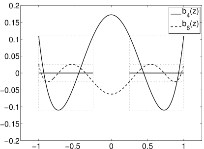
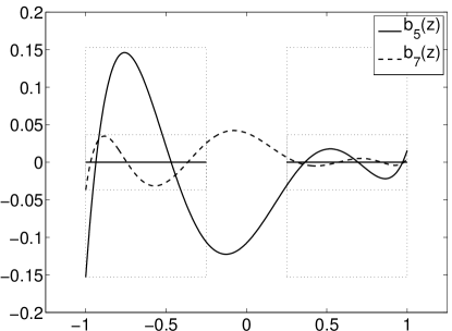
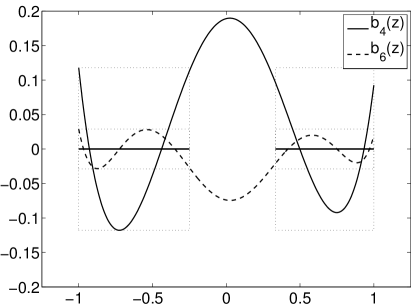
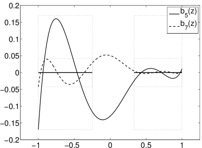
Using the series expansion (4.3)–(4.4) and the recurrence stated in Proposition 2.4, we can compute the Faber–Walsh polynomials for $E$ and the sequence $(\frac{D+C}{2},-\frac{D+C}{2},\frac{D+C}{2}$, $-\frac{D+C}{2},\ldots)$, were $\frac{D+C}{2}$ and $-\frac{D+C}{2}$ are the two foci of the lemniscatic domain $\mathcal{L}$ in (4.2). In Figure 1 we plot the polynomials $b_{k}$ for the set $E=[-1,-\frac{1}{4}]\cup[\frac{1}{4},1]$ and $k=4,6$ (left), $k=5,7$ (right). We observe that the polynomials of even degrees $k=4,6$ have $k+2$ extremal points on $E$. This suggests that they are the Chebyshev polynomials for $E$, i.e., that $b_{2k}(z)=T_{2k}(z;E)$, where, for all $j\geq 0$,

$$T_{j}(z;E)\mathrel{\mathop{:}}=\operatorname*{argmin}\{\|p\|_{E}:p\text{ monic and }\deg(p)=j\}$$

is the (uniquely determined) $j$th Chebyshev polynomial for the compact set $E$. We prove the following more general result, which for $n=2$ gives the result for two intervals.

Figure 1: Faber–Walsh polynomials $b_{k}$ for $E=[-1,-\frac{1}{4}]\cup[\frac{1}{4},1]$.

Theorem 4.2.

Let $E=\cup_{j=1}^{n}e^{i2\pi j/n}[C,D]$ with $0<C<D$. Then the Faber–Walsh polynomials $b_{nk}$ for $E$ and $(\alpha_{j})_{j=1}^{\infty}=\left(e^{i2\pi(j-1)/n}\left(\frac{D^{n/2}+C^{n/2}}{2}\right)^{n/2}\right)_{j=1}^{\infty}$ are the Chebyshev polynomials for $E$, i.e.,

$$b_{nk}(z)=T_{nk}(z;E),\quad k\geq 0.$$

Proof.

The result is trivial for $k=0$, so we may consider $k\geq 1$. The idea of the proof is to consider $E$ as a polynomial pre-image of $[-1,1]$ and to relate both the Faber–Walsh polynomial and the Chebyshev polynomial for $E$ to the Chebyshev polynomials of the first kind.

The polynomial

$$P(z)=\frac{2}{D^{n}-C^{n}}z^{n}-\frac{D^{n}+C^{n}}{D^{n}-C^{n}}=\frac{2z^{n}-C^{n}-D^{n}}{D^{n}-C^{n}},$$

satisfies $E=P^{-1}([-1,1])$, and the exterior Riemann map $\widetilde{\Phi}$ for $[-1,1]$ satisfies $\widetilde{\Phi}^{\prime}(\infty)=2$. Therefore, Theorem 3.3 shows that

$$b_{nk}(z)=\left(\frac{D^{n}-C^{n}}{4}\right)^{k}F_{k}(P(z)),\quad k\geq 0,$$

where $F_{k}$ is the $k$th Faber polynomial for $[-1,1]$. On the other hand, we have

$$T_{nk}(z;E)=\left(\frac{D^{n}-C^{n}}{2}\right)^{k}T_{k}(P(z);[-1,1])$$

from [15, Corollary 2.2]. For $k\geq 1$, the $k$th Chebyshev polynomial for $[-1,1]$ is

$$T_{k}(z;[-1,1])=\frac{1}{2^{k-1}}T_{k}(z),$$

where $T_{k}(z)$ is the $k$th Chebyshev polynomial of the first kind; see e.g. [14, Theorem 3.2.2]. Moreover, the $k$th Faber polynomial for $[-1,1]$ is given by $F_{k}(z)=2T_{k}(z)$ for $k\geq 1$; see [44, p. 37]. Thus

$$T_{nk}(z;E)=\left(\frac{D^{2}-C^{2}}{4}\right)^{k}2T_{k}(P(z))=\left(\frac{D^{2}-C^{2}}{4}\right)^{k}F_{k}(P(z))=b_{nk}(z),$$

which completes the proof. ∎

This theorem generalizes the classical relation of Faber and Chebyshev polynomials on the interval $[-1,1]$; see [44, p. 37]. For $n=2$ the statement of the theorem also holds for any two real intervals of equal length, which can be seen as follows. Let $E=[A,B]\cup[C,D]$ with $B-A=D-C>0$, and let $P(z)=z-\frac{B+C}{2}$. Then $\widetilde{E}=P(E)$ consists of two intervals of equal length which are symmetric with respect to the origin. If we denote the Faber–Walsh polynomials for $\widetilde{E}$ by $\widetilde{b}_{n}$, we find

$$b_{2k}(z)=\widetilde{b}_{2k}(P(z))=T_{2k}(P(z);\widetilde{E})=T_{2k}(z;E),$$

where we used Proposition 3.4, Theorem 4.2 and [15, Corollary 2.2].

In Proposition 3.6 we have shown that the normalized Faber–Walsh polynomials are asymptotically optimal. For sets $E$ of the form (4.1) this result can be strengthened as follows.

Corollary 4.3.

Let $E=[-D,-C]\cup[C,D]$ with $0<C<D$ and $z_{0}\in\mathbb{R}\backslash E$. Then the normalized Faber–Walsh polynomials for $E$ and $(\alpha_{j})_{j=1}^{\infty}=(\frac{D+C}{2},-\frac{D+C}{2},\frac{D+C}{2},-\frac{D+C}{2},\ldots)$ of even degree are optimal in the sense that

$$\frac{\|b_{2k}\|_{E}}{|b_{2k}(z_{0})|}=\min_{p\in\mathcal{P}_{2k}(z_{0})}\|p\|_{E},\quad k\geq 0.$$

Proof.

By Theorem 4.2, the Faber–Walsh polynomials of even degree are the Chebyshev polynomials for $E$. For $z_{0}\in\mathbb{R}\backslash[-D,D]$, Corollary 3.3.8 in [14] shows that the optimal polynomial is the normalized Chebyshev polynomial. For $z_{0}\in]-C,C[$, a little more work is required. First, it is not difficult to show that $T_{2}(z;E)=z^{2}-\frac{D^{2}+C^{2}}{2}$ with $\|T_{2}(z;E)\|_{E}=\frac{D^{2}-C^{2}}{2}$, and that $T_{2}(z;E)$ has the four extremal points $\pm C,\pm D$. Therefore, the optimal polynomial is the normalized Chebyshev polynomial; see [14, Corollary 3.3.6]. ∎

We point out that the argument in the previous proof is restricted to real $z_{0}$, since the proofs in [14] are based on the alternation property of the Chebyshev polynomials for subsets of the real line.

Note that the normalized Faber–Walsh polynomials $b_{k}(z)/b_{k}(z_{0})$ of odd degrees are not optimal: If $z_{0}\in\>]-C,C[$, it is known that the optimal polynomial is “defective”, i.e., the optimal polynomial for degree $2k+1$ is the same as for degree $2k$; see [14, Corollary 3.3.6]. If $z_{0}\in\mathbb{R}\backslash[-D,D]$, the optimal polynomial is the normalized Chebyshev polynomial ([14, Corollary 3.3.8]), while in general the Faber–Walsh polynomials of odd degree are not the Chebyshev polynomials, since they do not have $k+1$ extremal points on $E$ [14, Corollary 3.1.4]; see the example in Figure 1.

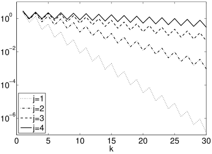
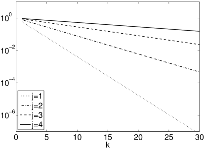
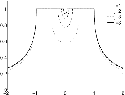
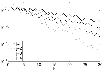
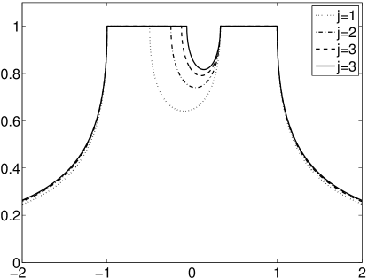
Let us continue with a numerical study of the maximum norm of the normalized Faber–Walsh polynomials, where we focus on the constraint point $z_{0}=0$. We compute the Faber–Walsh polynomials $b_{k,j}$, $k=1,2,\ldots$, for the sets

$$E_{j}\mathrel{\mathop{:}}=[-1,-2^{-j}]\cup[2^{-j},1],\quad j=1,2,3,4,$$ (4.6)

and the sequence $(\frac{D+C}{2},-\frac{D+C}{2},\frac{D+C}{2},-\frac{D+C}{2},\dots)$ using the coefficients of the Laurent series (4.3)–(4.4) and Proposition 2.4. Figure 2 (left) shows the values $\frac{\|b_{k,j}\|_{E_{j}}}{|b_{k,j}(0)|}$ of the normalized Faber–Walsh polynomials for the sets $E_{j}$. A comparison with the values $R_{0}(E_{j})^{k}$ shows that the actual convergence speed of $\frac{\|b_{k,j}\|_{E_{j}}}{|b_{k,j}(0)|}$ to zero almost exactly matches the rate predicted by the asymptotic analysis even for small values of $k$. Recall from (3.3) that $R_{z_{0}}(E)^{k}$ is a lower bound on $\|p\|_{E}$ for any $p\in\mathcal{P}_{k}(z_{0})$. The “zigzags” in the curves are due to the fact that for even degrees $b_{k,j}(z)/b_{k,j}(0)$ is the optimal polynomial (as shown in Corollary 4.3), while for odd degrees it is not.

Figure 2: The values $\frac{\|b_{k,j}\|_{E_{j}}}{|b_{k,j}(0)|}$ (left) and $R_{0}(E_{j})^{k}$ (right) for the sets $E_{j}$ from (4.6).

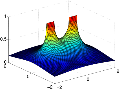
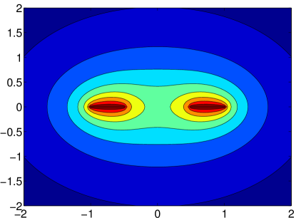
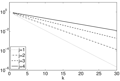
Let us discuss the asymptotic convergence factor of the set $E$ from (4.1). For two arbitrary real intervals and a real constraint point $z_{0}$, the asymptotic convergence factor can be expressed in terms of Jacobi’s elliptic and theta functions [2]; see also [14]. Estimates of the asymptotic convergence factor in terms of elementary functions have been derived in [38]. For the case of two intervals as in (4.1) and for an arbitrary real or complex constraint point $z_{0}\in\mathbb{C}\backslash E$, we have from (3.2) and Proposition 4.1

$$R_{z_{0}}(E)=\frac{\mu}{|U(\Phi(z_{0}))|}=\frac{1}{\sqrt{\frac{2}{D^{2}-C^{2}}\left|z_{0}^{2}-\frac{D^{2}+C^{2}}{2}\pm\sqrt{(z_{0}^{2}-C^{2})(z_{0}^{2}-D^{2})}\right|}},$$

where the sign of the square root is chosen to maximize the absolute value of the denominator. We thus obtain $R_{z_{0}}(E)$ in terms of elementary functions and for all complex $z_{0}\notin E$. For the special case $z_{0}=0$ we have $\Phi(0)=0$ and hence

$$R_{0}(E)=\sqrt{\frac{D-C}{D+C}}.$$

In Figure 3 we plot the asymptotic convergence factor $R_{z_{0}}([-1,-\frac{1}{2}]\cup[\frac{1}{2},1])$ as a function of $z_{0}\in\mathbb{C}$.

Figure 3: Asymptotic convergence factor $R_{z_{0}}([-1,-\frac{1}{2}]\cup[\frac{1}{2},1])$ as a function of $z_{0}\in\mathbb{C}$.

In Figure 4 we plot the asymptotic convergence factors $R_{z_{0}}(E_{j})$ for the sets $E_{j}$ of the form (4.6) and real $z_{0}$ ranging from $-2$ to $2$. Note that when $z_{0}$ is to the left or the right of the two intervals, i.e. $|z_{0}|>1$, the asymptotic convergence factors $R_{z_{0}}(E_{j})$ are almost identical for all $j$, and they decrease quickly with increasing $|z_{0}|$. On the other hand, when $z_{0}$ is between the two intervals the asymptotic convergence factors $R_{z_{0}}(E_{j})$ strongly depend on $j$, and for a fixed $z_{0}$ they increase quickly with increasing $j$. Moreover, $R_{z_{0}}(E_{j})$ for $|z_{0}|<2^{-j}$ is minimal when $z_{0}=0$, i.e., when $z_{0}$ is the midpoint between the two intervals.

Figure 4: Asymptotic convergence factors $R_{z_{0}}(E_{j})$ for $E_{j}$ from (4.6) and $z_{0}\in[-2,2]$.

4.2 Two arbitrary real intervals

In this section we consider the general case of two real intervals, i.e.,

$$E=[A,B]\cup[C,D]\quad\text{with }A<B<C<D.$$ (4.7)

For such sets, the lemniscatic map and lemniscatic domain are not known analytically. We therefore compute the map and the domain numerically using the method introduced in [32]. This methods needs as its input a discretization of the boundary of the set $E$, which is assumed to consist of Jordan curves. The numerical examples in [32] show that the method is efficient and works accurately even for domains with close-to-touching boundaries, non-convex boundaries, piecewise smooth boundaries, and of high connectivity.

We will apply two preliminary conformal maps in order to map $\widehat{\mathbb{C}}\backslash E$ for the set $E$ in (4.7) onto a domain bounded by Jordan curves. The preliminary maps are basically (inverse) Joukowski maps, as stated in the following lemma, which can be proven by elementary means.

Lemma 4.4.

Let $\alpha,\beta\in\mathbb{R}$ with $\alpha<\beta$. Then

$$\begin{split}\Phi&:\widehat{\mathbb{C}}\backslash[\alpha,\beta]\to\left\{w\in\widehat{\mathbb{C}}:\left|w-\frac{\beta+\alpha}{2}\right|>\frac{\beta-\alpha}{4}\right\},\\ &w=\Phi(z)=\frac{1}{2}\left(z+\frac{\beta+\alpha}{2}\pm\sqrt{(z-\alpha)(z-\beta)}\right),\end{split}$$

where we take the branch of the square root such that $|\Phi(z)-\frac{\beta+\alpha}{2}|>\frac{\beta-\alpha}{4}$, is a bijective conformal map which is normalized at infinity by $\Phi(z)=z+\mathcal{O}(1/z)$.

We now construct the lemniscatic map of $E=[A,B]\cup[C,D]$. The construction is illustrated in Figure 5 for the set $E=[-1,-h]\cup[h^{2},1]$ with $h=0.15$.

(a) Original domain $\mathcal{K}=\widehat{\mathbb{C}}\backslash E$

(b) $\mathcal{K}_{1}=\Phi_{1}(\mathcal{K})$

(c) $\mathcal{K}_{2}=\Phi_{2}(\mathcal{K}_{1})$

(d) Lemniscatic domain $\mathcal{L}=\Phi_{3}(\mathcal{K}_{2})$

Figure 5: Construction of the lemniscatic map of $[-1,-h]\cup[h^{2},1]$ with $h=0.15$.

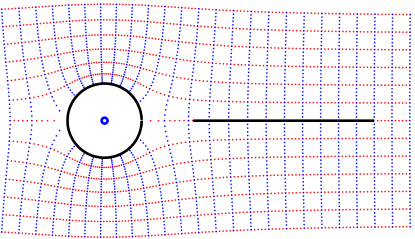
First we apply Lemma 4.4 to the interval $[A,B]$ to obtain the conformal map $\Phi_{1}$, mapping $\mathcal{K}$ onto $\mathcal{K}_{1}=\Phi_{1}(\mathcal{K})$, which is the exterior of

$$\{z_{1}:|z_{1}-w_{1}|=r_{1}\}\cup[\widetilde{C},\widetilde{D}],$$

with $w_{1}=\frac{B+A}{2}$, $r_{1}=\frac{B-A}{4}$, $\widetilde{C}=\Phi_{1}(C)$, and $\widetilde{D}=\Phi_{1}(D)$; see Figure 5(b). In a second step, let $\Phi_{2}$ be given by Lemma 4.4 for the interval $[\widetilde{C},\widetilde{D}]$. Then $\Phi_{2}$ maps $\mathcal{K}_{1}$ onto the exterior of

$$\Phi_{2}(\{z_{1}:|z_{1}-w_{1}|=r_{1}\})\cup\{z_{2}:|z_{2}-w_{2}|=r_{2}\},$$

where $w_{2}=\frac{\widetilde{D}+\widetilde{C}}{2}$ and $r_{2}=\frac{\widetilde{D}-\widetilde{C}}{4}$; see Figure 5(c). This domain is bounded by two analytic Jordan curves, which we parametrize by

$$\eta_{1}(t)=\Phi_{2}(w_{1}+r_{1}e^{-it})\quad\text{and}\quad\eta_{2}(t)=w_{2}+r_{2}e^{-it},\quad t\in[0,2\pi].$$ (4.8)

We then apply the numerical method from [32] to compute the lemniscatic domain $\mathcal{L}$ and lemniscatic map $\Phi_{3}$ of $\mathcal{K}_{2}=\Phi_{2}(\mathcal{K}_{1})$. As mentioned above, the input of this method is a discretization of the boundary, which is easily computable using the parameterization (4.8). The result is the lemniscatic map

$$\Phi\mathrel{\mathop{:}}=\Phi_{3}\circ\Phi_{2}\circ\Phi_{1}:\widehat{\mathbb{C}}\backslash E\to\mathcal{L},$$

where $\Phi_{1}$ and $\Phi_{2}$ are given analytically as above, and $\Phi_{3}$ is computed numerically. The output of the numerical method from [32] are the parameters of $\mathcal{L}$ and the boundary values of $\Phi_{3}$ at the discretization points on the boundary. The values of $\Phi_{3}$ at other points can be computed by Cauchy’s integral formula for domains with infinity as interior point, applied to the function $\Phi_{3}(z)-z$, which is analytic in $\mathcal{K}_{2}$ and vanishes at infinity. We thus have

$$\Phi_{3}(z)=z+\frac{1}{2\pi i}\int_{\partial\mathcal{K}_{2}}\frac{\Phi_{3}(\zeta)-\zeta}{\zeta-z}\,d\zeta,$$

where the boundary is parametrized such that $\mathcal{K}_{2}$ is to the left of the contour; see [32] for details on the practical computation of this integral. Note that this numerical method extends to any finite number of intervals.

With the lemniscatic map $\Phi$ and lemniscatic domain $\mathcal{L}$ available, we can compute the Faber–Walsh polynomials by

$$b_{k}(z)=\frac{1}{2\pi i}\int_{\gamma}\frac{u_{k}(\Phi(\zeta))}{\zeta-z}\,d\zeta=\frac{1}{2\pi i}\int_{\gamma}\frac{\prod_{j=1}^{k}(\Phi(\zeta)-\alpha_{j})}{\zeta-z}\,d\zeta,$$

see (2.6), where $\gamma$ is any positively oriented contour containing $E$ and $z$ in its interior, and where the sequence $(\alpha_{j})_{j=1}^{\infty}$ is chosen from the foci of the lemniscatic domain as indicated in the discussion below Lemma 2.2.

Figure 6 shows some computed Faber–Walsh polynomials of even (left) and odd (right) degrees for the set $E=[-1,-\frac{1}{4}]\cup[\frac{1}{3},1]$. Unlike in the case of two equal intervals, the Faber–Walsh polynomials for two unequal intervals are in general not Chebyshev polynomials, nor are the normalized Faber–Walsh polynomials the optimal polynomials. We numerically compute the Faber–Walsh polynomials $b_{k,j}$ for the sets

$$E_{j}\mathrel{\mathop{:}}=[-1,-2^{-j}]\cup[3^{-1},1],\quad j=1,2,3,4.$$ (4.9)

Figure 7 (left) shows the corresponding values $\|b_{k,j}\|_{E}/|b_{k,j}(0)|$ for $k=1,\ldots,30$. As for the equal intervals, a comparison with the values $R_{0}(E_{j})^{k}$ shows that the convergence speed to zero of the norms matches closely the predicted asymptotic rate, already for small values of $k$. Unlike in the case of two equal intervals, the sequence of norms has a few irregular jumps, which are due to the lack of symmetry in the problem. More precisely, all jumps happen when one of the foci $a_{1},a_{2}$ of the lemniscatic domain appears twice in a row in the sequence $(\alpha_{j})_{j=1}^{\infty}$. This happens in the construction of the sequence as described below Lemma 2.2, since for two unequal intervals the exponents $m_{1}$ and $m_{2}$ of the lemniscatic domain are different.

Figure 6: Faber–Walsh polynomials $b_{k}$ for $E=[-1,-\frac{1}{4}]\cup[\frac{1}{3},1]$.

Figure 7: The values $\frac{\|b_{k,j}\|_{E_{j}}}{|b_{k,j}(0)|}$ (left) and $R_{0}(E_{j})^{k}$ (right) for the sets $E_{j}$ from (4.9).

Finally, the numerical method from [32] yields the lemniscatic map $\Phi$, as well as the parameters of the lemniscatic domain $\mathcal{L}$. Therefore, the asymptotic convergence factor can be numerically computed by its characterization (3.2). In Figure 8 we plot the asymptotic convergence factor $R_{z_{0}}([-1,-\frac{1}{2}]\cup[\frac{1}{3},1])$ as a function of $z_{0}\in\mathbb{C}$.

Figure 8: Asymptotic convergence factor $R_{z_{0}}([-1,-\frac{1}{2}]\cup[\frac{1}{3},1])$ as a function of $z_{0}\in\mathbb{C}$.

In Figure 9 we plot the asymptotic convergence factors $R_{z_{0}}(E_{j})$ for the sets $E_{j}$ from (4.9) and real $z_{0}$ ranging from $-2$ to $2$. Similar remarks as in the case of two equal intervals apply, with one exception: Here the computation shows that $R_{z_{0}}(E_{j})$ for $z_{0}\in[-2^{-j},3^{-1}]$ attains its minimum not at the midpoint between the two intervals, but slightly to its left for $j=1$, and to its right for $j=2,3,4$. A similar observation has already been made by Fischer [14, Example 3.4.5].

Figure 9: Asymptotic convergence factors $R_{z_{0}}(E_{j})$ for $E_{j}$ from (4.9) and $z_{0}\in[-2,2]$.

5 Two non-real examples

In this section we give examples of Faber–Walsh polynomials for sets $E$ that are not subsets of the real line.

5.1 Two disks

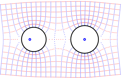
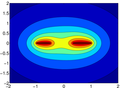
We consider sets $E$ consisting of two disks of the same radius, i.e.,

$$E=E(z_{0},r)\mathrel{\mathop{:}}=\{z\in\mathbb{C}:|z-z_{0}|\leq r\}\cup\{z\in\mathbb{C}:|z+z_{0}|\leq r\},$$

where we take $z_{0},r\in\mathbb{R}$ with $0<r<z_{0}$. The lemniscatic map of $E(z_{0},r)$ is known analytically from [41, Theorem 4.2], and the lemniscatic domain is of the form

$$\mathcal{L}=\mathcal{L}(z_{0},r)=\{w\in\widehat{\mathbb{C}}:|w-a_{1}|^{1/2}|w+a_{1}|^{1/2}>\mu\}$$

for some $a_{1}>0$ and $\mu>0$. With these $\mathcal{L}$ and $\Phi$ we obtain the Faber–Walsh polynomials for $E(z_{0},r)$ and $(a_{1},-a_{1},a_{1},-a_{1},\ldots)$ by their integral representation; see also the discussion in Section 4.2.

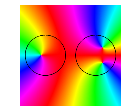
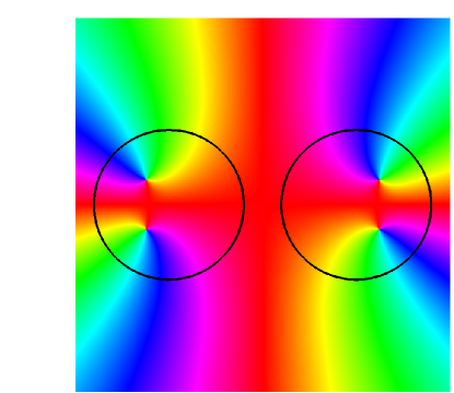
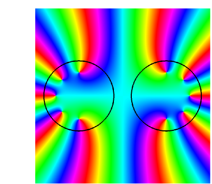
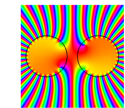
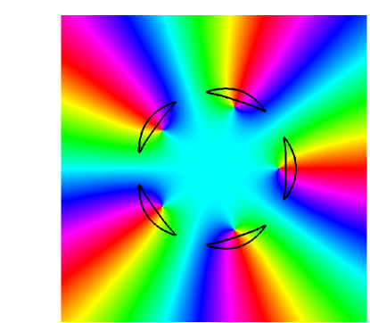
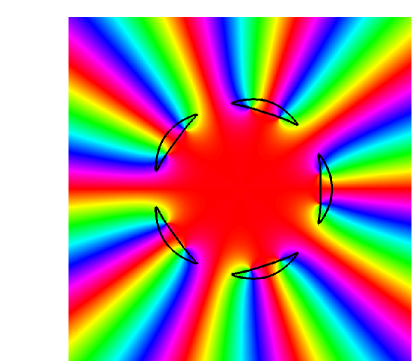
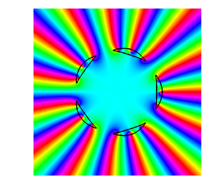
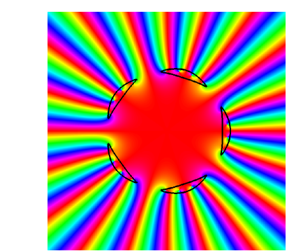
In Figure 10 we plot the phase portraits of several Faber–Walsh polynomials for $E(1,0.8)$; see [48, 49] for details on phase portraits. The figure shows that the $k$ roots of $b_{k}$ are all contained in $E$.

Figure 10: Phase portraits of Faber–Walsh polynomials $b_{k}$ for $E(1,0.8)$ for $k=3,4,10,40$.

We further compute the Faber–Walsh polynomials $b_{k,r}$ for the sets

$$E_{r}=E(1,r)\quad\text{for }r=0.5,0.7,0.9,$$ (5.1)

and the sequence $(a_{1},-a_{1},a_{1},-a_{1},\ldots)$. In Figure 11 (left) we plot the values $\frac{\|b_{k,r}\|_{E_{r}}}{|b_{k,r}(0)|}$ for $k=1,\ldots,30$.

Figure 11: The values $\frac{\|b_{k,r}\|_{E_{r}}}{|b_{k,r}(0)|}$ (left) and $R_{0}(E_{r})^{k}$ (right) for the sets $E_{r}$ from (5.1).

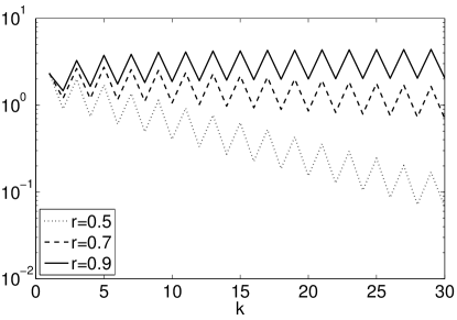
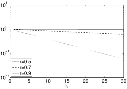
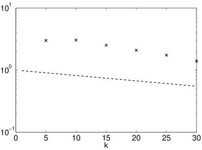
As in the case of two intervals, we observe that the convergence speed to zero of the norms almost exactly matches the rate predicted by the asymptotic analysis, already for small $k$. The numerically computed asymptotic convergence factors (rounded to five digits) for the three sets $E_{r}$ are $R_{0}(E_{0.5})=0.9099$, $R_{0}(E_{0.7})=0.9839$ and $R_{0}(E_{0.9})=0.9999$, which in particular explains the slow convergence to zero for $r=0.7$ and the (almost) stagnation for $r=0.9$.

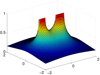
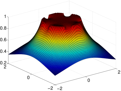
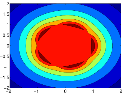
Figure 12 shows the numerically computed asymptotic convergence factor $R_{z_{0}}(E(1,0.7))$ as a function of $z_{0}\in\mathbb{C}$.

Figure 12: Asymptotic convergence factor $R_{z_{0}}(E(1,0.7))$ as a function of $z_{0}\in\mathbb{C}$.

5.2 A set with more components

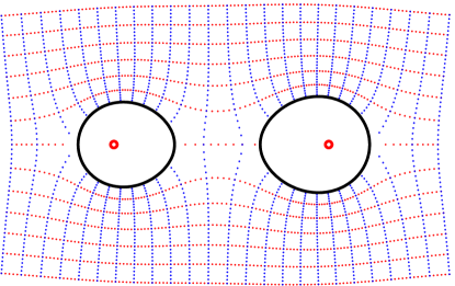
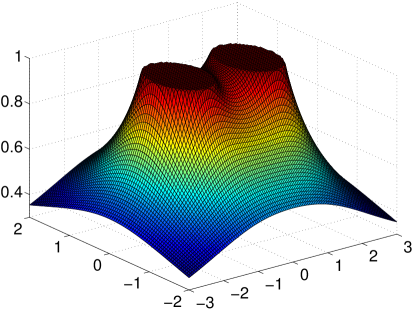
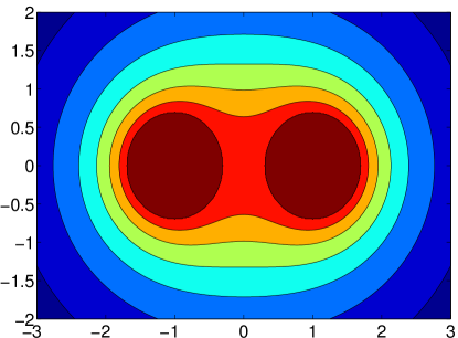
In this section we will give another illustration of Theorem 3.3, starting from a simply connected set of the form introduced in [24, Theorem 3.1]; see Figure 13(a) for an illustration.

Theorem 5.1 ([24, Theorem 3.1]).

Let $\lambda\in\mathbb{C}$ with $|\lambda|=1$, $\phi\in\>]0,2\pi[$ and $R\in[1,P[$, where

$$P\mathrel{\mathop{:}}=\tan(\phi/4)+\frac{1}{\cos(\phi/4)}.$$

Then $\Omega=\Omega(\lambda,\phi,R)$ is the compact set bounded by $\widetilde{\psi}(\{w\in\mathbb{C}:|w|=1\})$, where

$$\widetilde{\psi}(w)=\frac{(w-\lambda N)(w-\lambda M)}{(N-M)w+\lambda(NM-1)},\text{with }N=\frac{1}{2}\left(\frac{P}{R}+\frac{R}{P}\right),M=\frac{R^{2}-1}{2R\tan(\phi/4)},$$

is a bijective conformal map from the exterior of the unit circle onto $\widehat{\mathbb{C}}\backslash\Omega$ and satisfies $\widetilde{\psi}(\infty)=\infty$ and $\widetilde{\psi}^{\prime}(\infty)=t=1/(N-M)>0$. We further have $\lambda\notin\Omega$ and $\{\lambda e^{i\beta}:\phi/2\leq\beta\leq 2\pi-\phi/2\}\subseteq\Omega$.

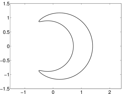
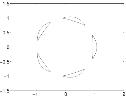
Let us consider polynomial pre-images of such sets. As an example we consider the set $\Omega=\Omega(-1,2\pi/3,1.1)$, which satisfies $\Omega=\Omega^{*}$. Let $E=P^{-1}(\Omega)$ with $P(z)=z^{n}$; see Figure 13(a) and 13(b) for an illustration with $n=5$. By Theorem 3.2, the lemniscatic domain corresponding to $E$ is

$$\mathcal{L}=\{w\in\widehat{\mathbb{C}}:|U(w)|=|w^{n}-tN|^{1/n}>t^{1/n}\},$$

where the logarithmic capacity $t$ of $\Omega$ is given as in Theorem 5.1. Since $tN>0$, the foci of the lemniscate are $a_{j}=e^{2\pi i\frac{j-1}{n}}(tN)^{1/n}$ for $j=1,2,\ldots,n$. By Theorem 3.3, the $(nk)$th Faber–Walsh polynomials for $E$ and

$$(a_{1},a_{2},\ldots,a_{n},a_{1},a_{2},\ldots,a_{n},\ldots)$$

are given by

$$b_{nk}(z)=t^{k}F_{k}(z^{n}),$$ (5.2)

where the $F_{k}$ are the Faber polynomials for $\Omega$, which are explicitly known from [24, Lemma 4.1]. There, the Faber polynomials are computed by a recursion involving all previous Faber polynomials. The Faber polynomials for $\Omega$ can also be computed by a short (three term) recursion; see [27].

(a) Set $\Omega=\Omega(-1,2\pi/3,1.1)$

(b) $E=P^{-1}(\Omega)$ with $P(z)=z^{5}$.

Figure 13: Set $\Omega=\Omega(-1,2\pi/3,1.1)$, its pre-image $E$, and phase portraits of Faber–Walsh polynomials for $E$ of degrees $k=5,10,15,20$.

The “missing” Faber–Walsh polynomials can be computed numerically using their definition (2.6), where we obtain the lemniscatic map $\Phi$ of $E$ from $\widetilde{\psi}^{-1}$ by Theorem 3.2. Note that $\widetilde{\psi}$ is a composition of two Möbius transformations and the Joukowski map, so that its inverse is easily computable; see [24, Theorem 3.1].

We plot the phase portraits of the Faber–Walsh polynomials $b_{5k}$ for $k=1,2,3,4$ in Figure 13. For degrees $5$ and $10$ we observe that not all zeros of the Faber–Walsh polynomial are in $E$, in contrast to the case of the two disks. This follows from the relation (5.2) and the fact that the zeros of the Faber polynomials $F_{1}$ and $F_{2}$ for $\Omega$ do not lie in $\Omega$; see [26] for details on these Faber polynomials. This also shows that the lower bound in (2.7) cannot, in general, hold for all $k$. In Figure 14 we plot the values $\|b_{5k}\|_{E}/|b_{5k}(0)|$ and, for comparison, the values $R_{0}(E)^{k}$, where $R_{0}(E)=0.9803$ (rounded to five digits).

Figure 14: The values $\frac{\|b_{k}\|_{E}}{|b_{k}(0)|}$ and $R_{0}(E)^{k}$.

From (3.2) and Theorem 3.2 the asymptotic convergence factor for $E$ and $z_{0}\in\mathbb{C}\backslash E$ is given by

$$R_{z_{0}}(E)=\frac{\mu}{|U(\Phi(z_{0}))|}=\frac{1}{|\widetilde{\Phi}(z_{0}^{n})|^{1/n}}.$$

Figure 15 shows the asymptotic convergence factor for $E$ as a function of $z_{0}\in\mathbb{C}$.

Figure 15: Asymptotic convergence factor $R_{z_{0}}(P^{-1}(\Omega))$ as a function of $z_{0}\in\mathbb{C}$, where $P(z)=z^{5}$ and $\Omega=\Omega(-1,2\pi/3,1.1)$.

Acknowledgements

We thank the anonymous referees for helpful comments.

References

- [1] N. I. Achieser, Theory of approximation, Translated by Charles J. Hyman, Frederick Ungar Publishing Co., New York, 1956.
- [2] N. Akhiezer, Über einige Funktionen, welche in zwei gegebenen Intervallen am wenigsten von Null abweichen. I., Bull. Acad. Sci. URSS, 1932 (1932), pp. 1163–1202.
- [3] , Über einige Funktionen, welche in zwei gegebenen Intervallen am wenigsten von Null abweichen. II., Bull. Acad. Sci. URSS, 1933 (1933), pp. 309–344.
- [4] B. Beckermann and L. Reichel, Error estimates and evaluation of matrix functions via the Faber transform, SIAM J. Numer. Anal., 47 (2009), pp. 3849–3883.
- [5] J. H. Curtiss, Faber polynomials and the Faber series, Amer. Math. Monthly, 78 (1971), pp. 577–596.
- [6] T. A. Driscoll, K.-C. Toh, and L. N. Trefethen, From potential theory to matrix iterations in six steps, SIAM Rev., 40 (1998), pp. 547–578.
- [7] M. Eiermann, On semiiterative methods generated by Faber polynomials, Numer. Math., 56 (1989), pp. 139–156.
- [8] M. Eiermann, X. Li, and R. S. Varga, On hybrid semi-iterative methods, SIAM J. Numer. Anal., 26 (1989), pp. 152–168.
- [9] M. Eiermann and W. Niethammer, On the construction of semi-iterative methods, SIAM J. Numer. Anal., 20 (1983), pp. 1153–1160.
- [10] M. Eiermann, W. Niethammer, and R. S. Varga, A study of semi-iterative methods for nonsymmetric systems of linear equations, Numer. Math., 47 (1985), pp. 505–533.
- [11] S. W. Ellacott, Computation of Faber series with application to numerical polynomial approximation in the complex plane, Math. Comp., 40 (1983), pp. 575–587.
- [12] , A survey of Faber methods in numerical approximation, Comput. Math. Appl. Part B, 12 (1986), pp. 1103–1107.
- [13] G. Faber, Über polynomische Entwickelungen, Math. Ann., 57 (1903), pp. 389–408.
- [14] B. Fischer, Polynomial based iteration methods for symmetric linear systems, Wiley-Teubner Series Advances in Numerical Mathematics, John Wiley & Sons, Ltd., Chichester; B. G. Teubner, Stuttgart, 1996.
- [15] B. Fischer and F. Peherstorfer, Chebyshev approximation via polynomial mappings and the convergence behaviour of Krylov subspace methods, Electron. Trans. Numer. Anal., 12 (2001), pp. 205–215.
- [16] H. Grunsky, Über konforme Abbildungen, die gewisse Gebietsfunktionen in elementare Funktionen transformieren. I, Math. Z., 67 (1957), pp. 129–132.
- [17] , Über konforme Abbildungen, die gewisse Gebietsfunktionen in elementare Funktionen transformieren. II, Math. Z., 67 (1957), pp. 223–228.
- [18] , Lectures on theory of functions in multiply connected domains, Vandenhoeck & Ruprecht, Göttingen, 1978.
- [19] M. Hasson, The capacity of some sets in the complex plane, Bull. Belg. Math. Soc. Simon Stevin, 10 (2003), pp. 421–436.
- [20] , The degree of approximation by polynomials on some disjoint intervals in the complex plane, J. Approx. Theory, 144 (2007), pp. 119–132.
- [21] V. Heuveline and M. Sadkane, Arnoldi-Faber method for large non-Hermitian eigenvalue problems, Electron. Trans. Numer. Anal., 5 (1997), pp. 62–76.
- [22] J. A. Jenkins, On a canonical conformal mapping of J. L. Walsh, Trans. Amer. Math. Soc., 88 (1958), pp. 207–213.
- [23] S. Kamo and P. Borodin, Chebyshev polynomials for Julia sets., Mosc. Univ. Math. Bull., 49 (1994), pp. 44–45.
- [24] T. Koch and J. Liesen, The conformal “bratwurst” maps and associated Faber polynomials, Numer. Math., 86 (2000), pp. 173–191.
- [25] H. J. Landau, On canonical conformal maps of multiply connected domains, Trans. Amer. Math. Soc., 99 (1961), pp. 1–20.
- [26] J. Liesen, On the location of the zeros of Faber polynomials, Analysis (Munich), 20 (2000), pp. 157–162.
- [27] , Faber polynomials corresponding to rational exterior mapping functions, Constr. Approx., 17 (2001), pp. 267–274.
- [28] A. I. Markushevich, Theory of functions of a complex variable. Vol. I, Prentice-Hall Inc., Englewood Cliffs, N.J., 1965.
- [29] , Theory of functions of a complex variable. Vol. III, Prentice-Hall, Inc., Englewood Cliffs, N.J., 1967.
- [30] I. Moret and P. Novati, The computation of functions of matrices by truncated Faber series, Numer. Funct. Anal. Optim., 22 (2001), pp. 697–719.
- [31] , An interpolatory approximation of the matrix exponential based on Faber polynomials, J. Comput. Appl. Math., 131 (2001), pp. 361–380.
- [32] M. M. S. Nasser, J. Liesen, and O. Sète, Numerical computation of the conformal map onto lemniscatic domains, Comput. Methods Funct. Theory, (2016), pp. 1–27.
- [33] F. Peherstorfer, Inverse images of polynomial mappings and polynomials orthogonal on them, in Proceedings of the Sixth International Symposium on Orthogonal Polynomials, Special Functions and their Applications (Rome, 2001), vol. 153, 2003, pp. 371–385.
- [34] F. Peherstorfer and K. Schiefermayr, Description of extremal polynomials on several intervals and their computation. I, II, Acta Math. Hungar., 83 (1999), pp. 27–58, 59–83.
- [35] F. Peherstorfer and R. Steinbauer, Orthogonal and -extremal polynomials on inverse images of polynomial mappings, J. Comput. Appl. Math., 127 (2001), pp. 297–315.
- [36] T. Ransford, Potential theory in the complex plane, vol. 28 of London Mathematical Society Student Texts, Cambridge University Press, Cambridge, 1995.
- [37] K. Schiefermayr, A lower bound for the minimum deviation of the Chebyshev polynomial on a compact real set, East J. Approx., 14 (2008), pp. 223–233.
- [38] , Estimates for the asymptotic convergence factor of two intervals, J. Comput. Appl. Math., 236 (2011), pp. 28–38.
- [39] , A lower bound for the norm of the minimal residual polynomial, Constr. Approx., 33 (2011), pp. 425–432.
- [40] O. Sète, Some properties of Faber–Walsh polynomials, ArXiv e-prints: 1306.1347v1, (2013).
- [41] O. Sète and J. Liesen, On conformal maps from multiply connected domains onto lemniscatic domains, Electron. Trans. Numer. Anal., 45 (2016), pp. 1–15.
- [42] V. I. Smirnov and N. A. Lebedev, Functions of a complex variable: Constructive theory, Translated from the Russian by Scripta Technica Ltd, The M.I.T. Press, Cambridge, Mass., 1968.
- [43] G. Starke and R. S. Varga, A hybrid Arnoldi-Faber iterative method for nonsymmetric systems of linear equations, Numer. Math., 64 (1993), pp. 213–240.
- [44] P. K. Suetin, Series of Faber polynomials, vol. 1 of Analytical Methods and Special Functions, Gordon and Breach Science Publishers, Amsterdam, 1998.
- [45] J. L. Walsh, On the conformal mapping of multiply connected regions, Trans. Amer. Math. Soc., 82 (1956), pp. 128–146.
- [46] , A generalization of Faber’s polynomials, Math. Ann., 136 (1958), pp. 23–33.
- [47] , Interpolation and approximation by rational functions in the complex domain, Fifth edition, American Mathematical Society, Providence, R.I., 1969.
- [48] E. Wegert, Visual Complex Functions, Birkhäuser/Springer Basel AG, Basel, 2012.
- [49] E. Wegert and G. Semmler, Phase plots of complex functions: a journey in illustration, Notices Amer. Math. Soc., 58 (2011), pp. 768–780.