Selection bias when using instrumental variable methods to compare two treatments but more than two treatments are available
Abstract
Instrumental variable (IV) methods are widely used to adjust for the bias in estimating treatment effects caused by unmeasured confounders in observational studies. In this manuscript, we provide empirical and theoretical evidence that the IV methods may result in biased treatment effects if applied on a data set in which subjects are preselected based on their received treatments. We frame this as a selection bias problem and propose a procedure that identifies the treatment effect of interest as a function of a vector of sensitivity parameters. We also list assumptions under which analyzing the preselected data does not lead to a biased treatment effect estimate. The performance of the proposed method is examined using simulation studies. We applied our method on The Health Improvement Network (THIN) database to estimate the comparative effect of metformin and sulfonylureas on weight gain among diabetic patients.
keywords:
Causal inference, Instrumental Variables, Selection Bias, Sensitivity Analysis.1 Introduction
Confounder adjustment is critical in the estimation of treatment effect in observational studies. In practice, however, there is no guarantee that all the confounders (i.e., baseline variables that affect both the treatment and outcome) have been measured. These unmeasured confounders can bias the treatment effect estimation.
Instrumental variable (IV) methods are designed to adjust for the bias caused by unmeasured confounders in estimating a difference measure of effect such as the risk difference. IVs are predictors of treatment allocation that are independent of unmeasured confounders and do not have a direct effect on the outcome (i.e., only affect the outcome through affecting the treatment). Intuitively, the IV method seeks to extract variation in treatment that is free of unmeasured confounders and uses this variation to estimate the treatment effect. For more information on IV methods, see Angrist et al. (1996), Newhouse and McClellan (1998), Greenland (2000), Hernán and Robins (2006), Cheng et al. (2009a), Baiocchi et al. (2014) and Imbens (2014). This paper is motivated by provider preference IV (PP IV) which is commonly used as an IV in health studies. PP IV utilizes the natural variation in medical practices to construct an IV. For example, in studying the effect of cyclooxygenase-2 (COX-2) inhibitors vs. nonselective nonsteroidal anti-inflammatory drugs (nonselective NSAIDs) on gastrointestinal complications Brookhart et al. (2006) used whether a patient’s physician last prescription for a patient prescribed a nonsteroidal anti-inflammatory drug (NSAID) was for a Cox-2 inhibitor or a nonselective NSAID as an IV for whether the patient was prescribed a Cox-2 inhibitor or a nonselective NSAID. Other examples of PP IV can be found in Brooks et al. (2003) and Brookhart and Schneeweiss (2007).
For a binary IV and binary treatment, Angrist et al. (1996) proposed a nonparametric estimator which identifies the treatment effect among subjects who would take the treatment if encouraged to do so by the IV and not take the treatment if not encouraged to do so by the IV (compliers). This estimator is equivalent to a 2 stage least square (2SLS) estimator where at the first stage the treatment is regressed on IV and at the second stage the outcome is regressed on fitted values of the first stage regression (i.e., predicted value of the treatment variable given the IV). The coefficient of the independent variable of the second stage regression is equivalent to the estimator proposed by Angrist et al. (1996). The 2SLS estimator is also called the Wald estimator after Wald (1940). More efficient versions of the 2SLS estimator has been developed by Imbens and Rubin (1997b), Imbens and Rubin (1997a) and Cheng et al. (2009b).
Although treatment effect estimation using IV approaches for binary treatments is straightforward, it is challenging when there are more than two treatment arms. In fact, Cheng and Small (2006) shows that the treatment effects are not point identifiable and proposes bounds on treatment effects using method of moments. Long et al. (2010) studies the same problem and proposes a Bayesian approach for finding credibility intervals for the identification region.
Sometimes investigators are interested in comparing the effect of two treatments while the data consist of more than two treatment options for patients. In this situation a common approach is to select patients who are assigned to the treatments of interest and perform the standard IV approach for binary treatment and IV to estimate the treatment effect (Hadley et al., 2003; Basu et al., 2007; Hadley et al., 2010; Suh et al., 2012; Chen et al., 2014).
The objective of this manuscript is to provide empirical and theoretical evidence that, in general, excluding patients based on their assigned treatment can result in selection bias. This problem has also been discussed in an independent work by Swanson (2014a), Swanson (2014b), and Swanson et al. (2015). In the current manuscript, we formalize the mechanism of this selection bias within a principal stratification framework and provide a procedure that identifies the treatment effect of interest as a function of a vector of sensitivity parameters. Specifically, the sensitivity parameters are used to estimate the probability of being assigned to one of the treatments of interest as a function of the observed outcome and the IV value (Gilbert et al., 2003). We also list assumptions under which selecting patients based on their received treatment does not lead to a biased treatment effect estimate.
The manuscript is organized as follows. Section 2 provides the setup and defines the causal estimand. It also lists the required assumptions for our procedure. In Section 3, we discuss the selection bias issue and present the proposed sensitivity analysis method. We report on the results of a simulation study in Section 4, where we examine the performance of our proposed method. In Section 5, we study the comparative effect of metformin and sulfonylureas on weight gain using The Health Improvement Network (THIN) database.
2 Settings and Notations
For simplicity we focus on observational studies with three treatment options A, B, and C. We assume that we are only interested in comparing the effect of treatment A with B. We use small letters to refer to the possible values of the corresponding capital letter random variable. Let be a binary instrumental variable where such as provider preference. means that the IV predisposes the patient to receive treatment level among the options and , and means that the IV predisposes the patient to receive treatment level among the options and ; e.g., in Brookhart et al. (2006) study, if A denotes Cox-2 inhibitor and denotes nonselective NSAID, if the patient’s physician last prescription to a patient prescribed an NSAID was a Cox-2 inhibotor and if it was a nonselective NSAID. Let be the potential treatment assigned given , where , i.e., is the treatment that would be received if the IV was . The potential outcomes are for and , i.e., is the outcome that would be observed if the IV was and the treatment level was . The observed treatment and outcome are and , respectively.
Frangakis and Rubin (2002) developed a basic principal strata (PS) framework which stratifies subjects based on their potential assigned treatments. In our setting, we can classify subjects into the following 9 principal strata: ) always B taker, ) always A taker, ) always C taker, ) subjects who would comply with their value of instrumental variable, i.e., , , ) subjects who would take B if and would take C if , ) subjects who would take C if and would take A if , ) subjects who would take A if and would take B if , ) subjects who would take B if and would take C if , and ) subjects who would take A if and would take C if . We denote the proportions in the basic principal strata as .
We assume that the IV satisfies the following standard assumptions (Angrist et al., 1996): 1) stable unit treatment value assumption, 2) The IV is independent of unmeasured confounders, potential outcomes and potential treatment received, 3) the IV affects the treatment but has no direct effect on the outcome. This assumption is known to as the exclusion restriction (ER) assumption. Under the exclusion restriction, we let be the potential outcome if treatment is received which equal , and 4) the IV is independent of the pretreatment covariates, potential outcome and potential treatments. Furthermore, we assume two types of monotonicity assumptions: 5) monotonicity I: there is no defiers (i.e., ) and 6) monotonicity II: there is no one who would take if but take if and no one who would take if but take if . Note that monotonicity assumptions 5 & 6 reduce the number of principal strata to 6. The parameter of interest is defined as
3 IV Selection Bias
We show in this manuscript that IV analysis methods may not result in an unbiased treatment effect if applied on a data set in which units are preselected based on their received treatments. A standard IV analysis of patients on the subset of patients for whom or is essentially a comparison of the vs. patients on this subset. If has a different effect on whether than , then there will be selection bias. For example, patients who are in a more severe stages of the disease may be treated with treatment and therefore have less chance to be observed in the sample; if doctors who prefer drug are more likely to use treatment with severe patients than doctors who prefer drug , then there will be selection bias. Another scenario where such selection bias might arise is that treatment is more likely to be offered if some complications are present and doctors who prefer drug are more likely to treat a patient with complications with drug than doctors who prefer drug .
The challenge is that is not identifiable using the observed data when there is selection bias. This is due to the fact that the observed outcomes of is a mixture of potential outcomes from principal strata. Let be the density of outcome for a patient who received when assigned to (i.e., ). Then
where and is the density function of the outcome for subjects in principal stratum with . The density and can be written as
Thus,
| (1) |
Similarly, let be the density of outcome for a patient who received when assigned to . Then
where and is the density function of the outcome for subjects in principal stratum with . Also,
Thus,
| (2) |
The mixture proportions and are unknown and need to be estimated using the observed data. However, the strata proportions are not identifiable using the proportions in the observable strata, because
| (3) |
does not have a unique solution. Also, the density functions and are not identifiable using the observed data because , , and are unknown. So we assume logit models for these probabilities and perform the sensitivity analysis based on these models;
| (4) | ||||
| (5) |
Note that for any fixed (), () can be determined since and . Therefore, the parameter of interest can be estimated using the four dimensional sensitivity parameter (.
Remark. If it is plausible to assume that at least one of the principal strata , or is empty, we can reduce the dimension of the sensitivity parameters to two by estimating and using the observed data.
3.1 No Selection Bias
Let be a binary variable which is 1 if a patient is assigned to one of the treatments of interest and 0 otherwise. Under either of the following two conditions, the treatment effect is identifiable when we have access to the entire data (i.e., data includes patients who have received treatment C as well as A and B):
-
A.1
where and are measured and unmeasured confounders, respectively.
-
A.2
.
Assumption A.1 implies that the IV is unrelated to the patient’s selection. In other words, a patient would have the same chance of being selected for both values of the IV. A.2 means that the selection probability is independent of the unmeasured confounders given the instrumental variable and measured confounders. Figure 1 depicts the association between different variables. The left plot presents a scenario in which analyzing the preselected data will cause bias because conditioning on will open the path which violates one of the IV assumptions. This path is closed under either of assumptions A.1 or A.2 as shown in the center and right plots, respectively.
Under either of assumptions A.1 or A.2, the treatment effect can be identified. Specifically, under assumption A.1, the principal strata and does not exist. Thus
These equations can be used to identify . Also, under assumption A.2, can be estimated using the following three-step procedure:
-
Step1.
Using the entire data, estimate by postulating a logit model on .
-
Step2.
Include patients who have been assigned to either treatments A or B.
-
Step3.
Estimate the treatment effect using 2SLS IV approach. At each stage fit a weighted least square where weights are .
Fitting weighted least squares accounts for the selection procedure and hence avoids the bias by creating a pseudo-population in which there is no association between and .
3.2 Inference Procedure
Let and denote the outcome of patients whose received treatment matches their IV value for and , respectively. We assume that samples are independent within and between each IV group and identically distributed within each group.
For any fixed , is defined as a solution to
where and are empirical distributions calculated from the observed samples and . These equations can be solved using a one dimensional grid search on real line.
4 Simulation Studies
Through simulations we examine the performance of our proposed sensitivity analysis assuming known and unknown . We assume two scenarios with the following principal strata proportions: Scenario 1:
-
•
Scenario 1: , and which gives us .
-
•
Scenario 2: , , and which gives us .
The true amount of selection bias is determined by the parameters and in (4) and (5), respectively. The outcome of individuals with and are generated from a normal distribution with mean 2.5 and standard error 2 (i.e., ). Also, the outcome of individuals with and are generated from a normal distribution with mean and standard error 2 (i.e., ). For each set of , the parameter is determined such that the true treatment effect among compliers is , 0.50 and 0.80. We generate samples using rejection sampling from densities and according to (1) and (2), respectively.
Table 1 presents the statistical power of detecting the true treatment effect , 0.50, and 0.80 based on 500 datasets of sizes n=500 with , (1,1) and (0,0). The nominal type-I error rate is 5%. For both scenarios when the true amount of selection bias is presumed, the empirical and nominal sizes are close. In general, the empirical sizes are inflated when the selection bias parameters are not set correctly. For some of the combinations of the true and presumed sensitivity parameter values the power and type-I error rate are much higher than the nominal one which is caused by the overestimation of the treatment effect. Also, in scenario 2, when there is no selection bias (i.e., true ) and we presumed the power is very low because of the underestimation of the treatment effect. Table 2 shows the bias (), standard error and mean squared error of the treatment effect estimation for different combinations of the true and presumed sensitivity parameters when the true treatment effect . This table highlights the over- and underestimation phenomenon discussed earlier. Specifically, when the true sensitivity parameters are , presuming will result in underestimating the counterfactual mean outcome . This is because when we set the presumed less than the true value, the larger outcomes are less likely to be a complier among patients with . In other words it will shift the distribution of this compliers to left. Similarly when the presumed more than the true value, will be overestimated (See rows 3 and 4 in Table 2).
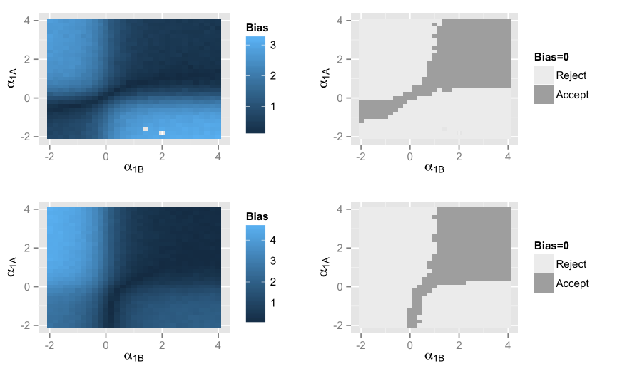
Figure 2 shows how the treatment effect estimate changes by the sensitivity parameters when the true and . The darker area in left panel of Figure 2 indicates the smaller bias and the darker area in the right panel shows the region in which the bias is not significant at (i.e., the confidence interval for contains zero). See also Table 2.

| Scenario 1 | Scenario 2 | ||||||
|---|---|---|---|---|---|---|---|
| True | Presumed | 0.00 | 0.50 | 0.80 | 0.00 | 0.50 | 0.80 |
| (1,2) | (1,2) | 0.04 | 0.60 | 0.91 | 0.04 | 0.52 | 0.86 |
| (1,2) | (1,1) | 0.12 | 0.81 | 0.98 | 0.22 | 0.88 | 0.97 |
| (1,2) | (0,0) | 0.16 | 0.36 | 0.78 | 0.99 | 1.00 | 1.00 |
| (1,1) | (1,1) | 0.05 | 0.58 | 0.91 | 0.05 | 0.48 | 0.85 |
| (1,1) | (2,2) | 0.08 | 0.71 | 0.95 | 0.10 | 0.24 | 0.61 |
| (1,1) | (0,0) | 0.35 | 0.05 | 0.40 | 0.90 | 1.00 | 1.00 |
| (0,0) | (0,0) | 0.04 | 0.61 | 0.92 | 0.05 | 0.60 | 0.94 |
| (0,0) | (1,0) | 1.00 | 1.00 | 1.00 | 0.80 | 1.00 | 1.00 |
| (0,0) | (1,1) | 0.34 | 0.96 | 1.00 | 0.81 | 0.00 | 0.03 |
| Scenario 1 | Scenario 2 | ||||||
|---|---|---|---|---|---|---|---|
| True | Presumed | Bias | S.D. | MSE | Bias | S.D. | MSE |
| (1,2) | (1,2) | -0.01 | 0.28 | 0.08 | 0.01 | 0.30 | 0.09 |
| (1,2) | (1,1) | -0.22 | 0.29 | 0.14 | -0.38 | 0.32 | 0.25 |
| (1,2) | (0,2) | 1.38 | 0.25 | 1.97 | 0.81 | 0.29 | 0.74 |
| (1,2) | (1,0) | -1.18 | 0.25 | 1.43 | -2.17 | 0.28 | 4.82 |
| (1,2) | (0,0) | 0.21 | 0.23 | 0.10 | -1.34 | 0.25 | 1.86 |
| (1,1) | (1,1) | 0.00 | 0.28 | 0.08 | -0.01 | 0.30 | 0.10 |
| (1,1) | (1,2) | 0.19 | 0.28 | 0.11 | 0.39 | 0.31 | 0.26 |
| (1,1) | (0,2) | 1.58 | 0.27 | 2.58 | 1.17 | 0.30 | 1.49 |
| (1,1) | (1,0) | -0.98 | 0.26 | 1.02 | -1.77 | 0.28 | 3.20 |
| (1,1) | (0,0) | 0.41 | 0.23 | 0.23 | -0.95 | 0.27 | 0.98 |
| Presumed | Scenario 1 | Scenario 2 | ||||
|---|---|---|---|---|---|---|
| 0.00 | 0.50 | 0.80 | 0.00 | 0.50 | 0.80 | |
| (0.3,0.6,1,2) | 0.38 | 0.90 | 0.98 | 1.00 | 1.00 | 1.00 |
| (0.3,0.6,0,2) | 1.00 | 0.00 | 0.00 | 0.07 | 0.73 | 0.96 |
| (0.3,0.6,1,0) | 1.00 | 1.00 | 1.00 | 1.00 | 1.00 | 1.00 |
| (0.3,0.6,0,0) | 0.12 | 0.35 | 0.80 | 1.00 | 1.00 | 1.00 |
| (0.5,0.5,1,2) | 0.40 | 0.08 | 0.38 | 0.93 | 1.00 | 1.00 |
| (0.5,0.5,0,2) | 1.00 | 0.00 | 0.00 | 0.04 | 0.40 | 0.75 |
| (0.5,0.5,1,0) | 0.96 | 1.00 | 1.00 | 1.00 | 1.00 | 1.00 |
| (0.5,0.5,0,0) | 0.10 | 0.29 | 0.76 | 1.00 | 1.00 | 1.00 |
| (0.2,0.8,1,2) | 0.98 | 1.00 | 1.00 | 1.00 | 1.00 | 1.00 |
| (0.2,0.8,0,2) | 0.94 | 0.00 | 0.05 | 0.61 | 1.00 | 1.00 |
| (0.2,0.8,1,0) | 1.00 | 1.00 | 1.00 | 1.00 | 1.00 | 1.00 |
| (0.2,0.8,0,0) | 0.06 | 0.24 | 0.65 | 1.00 | 1.00 | 1.00 |
| (0.7,0.2,1,2) | 1.00 | 0.00 | 0.00 | 0.30 | 0.08 | 0.32 |
| (0.7,0.2,0,2) | 1.00 | 0.00 | 0.00 | 0.98 | 0.00 | 0.00 |
| (0.7,0.2,1,0) | 0.65 | 0.99 | 1.00 | 1.00 | 1.00 | 1.00 |
| (0.7,0.2,0,0) | 0.12 | 0.39 | 0.87 | 1.00 | 1.00 | 1.00 |
4.1 Unknown
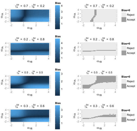
In this case our sensitivity parameter space is . Figures 3 and 4 present the bias in the treatment effect estimation for different values of the presumed sensitivity parameters based on scenarios 1 and 2, respectively. In these figures the true and in scenarios 1 and 2, respectively. Also the true treatment effect is . The darker area in the left panel shows the region in the sensitivity parameter space in which the bias is smaller and right panel shows the area in which the bias is not significant based on 500 samples (i.e., the confidence interval for contains zero). The shape of the area which leads to an unbiased estimate changes by the value of the presumed and, in general, when the presumed values of are far from the true values, the unbiased area is small which means it would be less likely to find an unbiased treatment effect estimate using sensitivity analysis (see also Table 4 in Appendix A). We have tabulated the power and type-I error rate for different values of the presumed sensitivity parameters in Table 3. This Table summarizes the result for three different values of the true treatment effect , and 0.80. The nominal type-I error rate is 5%.
5 Application to Real Data
The Health Improvement Network (THIN) is a large database, which contains the electronic medical record of more than 11 million patients. The data contains longitudinal measurements of diagnostic and prescription data and baseline characteristics collected from over 500 general practices in the UK. We are interested in assessing the effect of metformin and sulfonylureas on body mass index (BMI, calculated as mass in kilograms divided by the square of height in meters) among diabetic patients. Our focus is on patients who are taking these treatments as an initial treatment and the BMI is measured two years after treatment initiation. In our analysis we coded metformin and sulfonylureas as and , respectively.
In the modern era, metformin is universally acknowledged as the appropriate first-line medication for diabetes type 2 except where contraindicated (Nathan et al., 2009). While this dominance was being established in the late 1990s and early 2000s, sulfonylureas were the competing first line agent. During that time the prevalence of metformin use in clinical practice rose very quickly, at the expense of sulfonylureas.
The dynamic aspect of the preference justifies the use of provider preference as an IV. We define the preference as a time-varying quantity such that for each practice ID, the IV is defined as an average of metformin use during each two year timeframe from 1998 to 2012. We assign if the average is more than 50% and otherwise. Thus, a particular practice ID may have for one period of time and for the other.
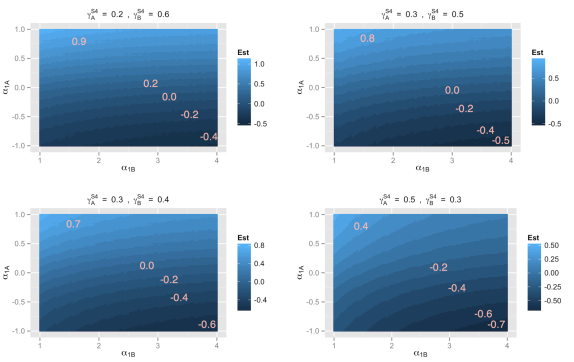
Our data includes patients who have been assigned to medications other than metformin or sulfonylureas as an initial therapy. Figure 5 presents the sensitivity analysis for the estimation of the treatment effect of interest based on a four dimensional sensitivity parameter . The parameter identifies the probability that a patient with a particular value of BMI would have taken if (i.e., seeing a physician with sulfonylureas preference) given that she has taken with (i.e., seeing a physician with metformin preference). The parameter has a similar interpretation and the parameter () is defined as a chance of being a complier for patients who have been assigned to and have taken . Since the association of sulfonylureas with weight gain is known it makes sense to assume that the true value of the parameter should be negative and should be positive. Also on average patients who have taken sulfonylureas () given are more likely to be compliers compare with those who have taken metformin () given . This means that it is very likely that .
The range of the treatment effect estimate varies by different choices of and . Specifically, for and , the treatment effect lies in ; while for and , it lies in . Based on our sensitivity analysis, it is unlikely that metformin be associated with increase in BMI and a large negative effect (i.e., ) is also unlikely because it requires very small and large values of and , respectively. Hence, if anything, the treatment effect of interest should lie in .
6 Discussion
This manuscript shows that IV analysis methods may fail to provide an unbiased estimate of treatment effects when analyzing data in which subjects are selected based on their received treatment. Specifically, this selection bias happens if the chance of including patients in the preselected data varies based on their IV value and/or some unmeasured confounders. For example, suppose we are interested in studying the comparative effect of treatment and while there is a third choice of treatment . Suppose patients with more severe stages of the disease are more likely to be treated with if seeing a doctor with preference. Then if we analyzed a data that only includes patients who have received treatment or , severe cases will be under represented among patients who have seen doctors with preference. This means that in the preselected data, the IV is associated with an unmeasured confounder which makes the IV invalid and results in a biased treatment effect estimate.
Within the principal strata framework, we develop a sensitivity analysis that can be used to estimate the treatment effect among compliers as a function of a vector of sensitivity parameters. Specifically, the sensitivity parameters are used to identify the probability of being a complier given the IV value, received treatment and the observed outcome. The dimension of the sensitivity parameter can be reduced if it is plausible to assume that there is no always takers. This is because the proportions in the principal strata are identifiable which means and can be estimated using the observed data.
Acknowledgment
This work is partially supported by NSF grant SES-1260782.
Appendix
In this Appendix, we present the supplementary materials.
Appendix: A
Table 4 shows the bias (), standard error and mean squared error of the treatment effect estimation for different combinations of the true and presumed sensitivity parameters when the true treatment effect .
| Scenario 1 | Scenario 2 | |||||
|---|---|---|---|---|---|---|
| Presumed | Bias | S.D. | MSE | Bias | S.D. | MSE |
| (0.3,0.6,1,2) | -0.37 | 0.29 | 0.22 | -1.92 | 0.34 | 3.79 |
| (0.3,0.6,0,2) | 1.37 | 0.24 | 1.95 | -0.18 | 0.30 | 0.12 |
| (0.3,0.6,1,0) | -1.54 | 0.27 | 2.45 | -3.07 | 0.34 | 9.55 |
| (0.3,0.6,0,0) | 0.23 | 0.24 | 0.11 | -1.32 | 0.27 | 1.83 |
| (0.5,0.5,1,2) | 0.46 | 0.26 | 0.28 | -1.09 | 0.29 | 1.28 |
| (0.5,0.5,0,2) | 1.65 | 0.26 | 2.80 | 0.11 | 0.27 | 0.08 |
| (0.5,0.5,1,0) | -0.95 | 0.27 | 1.04 | -2.57 | 0.28 | 6.72 |
| (0.5,0.5,0,0) | 0.20 | 0.23 | 0.09 | -1.35 | 0.26 | 1.89 |
| (0.2,0.8,1,2) | -1.22 | 0.31 | 1.59 | -2.76 | 0.39 | 7.80 |
| (0.2,0.8,0,2) | 0.87 | 0.25 | 0.81 | -0.69 | 0.27 | 0.55 |
| (0.2,0.8,1,0) | -1.86 | 0.29 | 3.54 | -3.42 | 0.36 | 11.88 |
| (0.2,0.8,0,0) | 0.23 | 0.23 | 0.11 | -1.32 | 0.25 | 1.79 |
| (0.7,0.2,1,2) | 1.98 | 0.34 | 4.03 | 0.44 | 0.32 | 0.30 |
| (0.7,0.2,0,2) | 2.72 | 0.33 | 7.54 | 1.20 | 0.32 | 1.53 |
| (0.7,0.2,1,0) | -0.55 | 0.24 | 0.36 | -2.09 | 0.27 | 4.45 |
| (0.7,0.2,0,0) | 0.18 | 0.25 | 0.10 | -1.34 | 0.26 | 1.88 |
References
- Angrist et al. (1996) Angrist, J. D., G. W. Imbens, and D. B. Rubin (1996): “Identification of causal effects using instrumental variables,” Journal of the American statistical Association, 91, 444–455.
- Baiocchi et al. (2014) Baiocchi, M., J. Cheng, and D. S. Small (2014): “Tutorial in biostatistics: Instrumental variable methods for causal inference,” .
- Basu et al. (2007) Basu, A., J. J. Heckman, S. Navarro-Lozano, and S. Urzua (2007): “Use of instrumental variables in the presence of heterogeneity and self-selection: an application to treatments of breast cancer patients,” Health economics, 16, 1133–1157.
- Brookhart and Schneeweiss (2007) Brookhart, M. A. and S. Schneeweiss (2007): “Preference-based instrumental variable methods for the estimation of treatment effects: assessing validity and interpreting results,” The international journal of biostatistics, 3.
- Brookhart et al. (2006) Brookhart, M. A., P. Wang, D. H. Solomon, and S. Schneeweiss (2006): “Evaluating short-term drug effects using a physician-specific prescribing preference as an instrumental variable,” Epidemiology (Cambridge, Mass.), 17, 268.
- Brooks et al. (2003) Brooks, J. M., E. A. Chrischilles, S. D. Scott, and S. S. Chen-Hardee (2003): “Was breast conserving surgery underutilized for early stage breast cancer? instrumental variables evidence for stage ii patients from iowa,” Health services research, 38, 1385–1402.
- Chen et al. (2014) Chen, H., S. Mehta, R. Aparasu, A. Patel, and M. Ochoa-Perez (2014): “Comparative effectiveness of monotherapy with mood stabilizers versus second generation (atypical) antipsychotics for the treatment of bipolar disorder in children and adolescents,” Pharmacoepidemiology and drug safety, 23, 299–308.
- Cheng et al. (2009a) Cheng, J., J. Qin, and B. Zhang (2009a): “Semiparametric estimation and inference for distributional and general treatment effects,” Journal of the Royal Statistical Society: Series B (Statistical Methodology), 71, 881–904.
- Cheng and Small (2006) Cheng, J. and D. S. Small (2006): “Bounds on causal effects in three-arm trials with non-compliance,” Journal of the Royal Statistical Society: Series B (Statistical Methodology), 68, 815–836.
- Cheng et al. (2009b) Cheng, J., D. S. Small, Z. Tan, and T. R. Ten Have (2009b): “Efficient nonparametric estimation of causal effects in randomized trials with noncompliance,” Biometrika, 96, 19–36.
- Frangakis and Rubin (2002) Frangakis, C. E. and D. B. Rubin (2002): “Principal stratification in causal inference,” Biometrics, 58, 21–29.
- Gilbert et al. (2003) Gilbert, P. B., R. J. Bosch, and M. G. Hudgens (2003): “Sensitivity analysis for the assessment of causal vaccine effects on viral load in hiv vaccine trials,” Biometrics, 59, 531–541.
- Greenland (2000) Greenland, S. (2000): “An introduction to instrumental variables for epidemiologists,” International journal of epidemiology, 29, 722–729.
- Hadley et al. (2003) Hadley, J., D. Polsky, J. S. Mandelblatt, J. M. Mitchell, J. C. Weeks, Q. Wang, and Y.-T. Hwang (2003): “An exploratory instrumental variable analysis of the outcomes of localized breast cancer treatments in a medicare population,” Health economics, 12, 171–186.
- Hadley et al. (2010) Hadley, J., K. R. Yabroff, M. J. Barrett, D. F. Penson, C. S. Saigal, and A. L. Potosky (2010): “Comparative effectiveness of prostate cancer treatments: evaluating statistical adjustments for confounding in observational data,” Journal of the National Cancer Institute.
- Hernán and Robins (2006) Hernán, M. A. and J. M. Robins (2006): “Instruments for causal inference: an epidemiologist’s dream?” Epidemiology, 17, 360–372.
- Imbens (2014) Imbens, G. W. (2014): “Instrumental variables: An econometrician’s perspective,” Technical report, National Bureau of Economic Research.
- Imbens and Rubin (1997a) Imbens, G. W. and D. B. Rubin (1997a): “Bayesian inference for causal effects in randomized experiments with noncompliance,” The Annals of Statistics, 305–327.
- Imbens and Rubin (1997b) Imbens, G. W. and D. B. Rubin (1997b): “Estimating outcome distributions for compliers in instrumental variables models,” The Review of Economic Studies, 64, 555–574.
- Long et al. (2010) Long, Q., R. J. Little, and X. Lin (2010): “Estimating causal effects in trials involving multitreatment arms subject to non-compliance: a bayesian framework,” Journal of the Royal Statistical Society: Series C (Applied Statistics), 59, 513–531.
- Nathan et al. (2009) Nathan, D., J. Buse, M. Davidson, E. Ferrannini, R. Holman, R. Sherwin, and B. Zinman (2009): “American diabetes association; european association for study of diabetes. medical management of hyperglycemia in type 2 diabetes: a consensus algorithm for the initiation and adjustment of therapy: a consensus statement of the american diabetes association and the european association for the study of diabetes,” Diabetes care, 32, 193–203.
- Newhouse and McClellan (1998) Newhouse, J. P. and M. McClellan (1998): “Econometrics in outcomes research: the use of instrumental variables,” Annual review of public health, 19, 17–34.
- Suh et al. (2012) Suh, H. S., J. W. Hay, K. A. Johnson, and J. N. Doctor (2012): “Comparative effectiveness of statin plus fibrate combination therapy and statin monotherapy in patients with type 2 diabetes: use of propensity-score and instrumental variable methods to adjust for treatment-selection bias,” Pharmacoepidemiology and drug safety, 21, 470–484.
- Swanson (2014a) Swanson, R. J. M. M. . H. M., SA (2014a): “Selection bias in instrumental variable analyses comparing active treatments,” in Paper presented at the 47th Annual Meeting of the Society for Epidemiologic Research.
- Swanson (2014b) Swanson, S. (2014b): Contributions to instrumental variable methods in epidemiology, Ph.D. thesis, Harvard School of Public Health, Boston, MA.
- Swanson et al. (2015) Swanson, S. A., J. M. Robins, M. Miller, and M. A. Hernán (2015): “Selecting on treatment: A pervasive form of bias in instrumental variable analyses,” American Journal of Epidemiology, kwu284.
- Wald (1940) Wald, A. (1940): “The fitting of straight lines if both variables are subject to error,” The Annals of Mathematical Statistics, 11, 284–300.