Scaling law for crystal nucleation time in glasses

Abstract

Due to high viscosity, glassy systems evolve slowly to the ordered state. Results of molecular dynamics simulation reveal that the structural ordering in glasses becomes observable over “experimental” (finite) time-scale for the range of phase diagram with high values of pressure. We show that the structural ordering in glasses at such conditions is initiated through the nucleation mechanism, and the mechanism spreads to the states at extremely deep levels of supercooling. We find that the scaled values of the nucleation time, $\tau_{1}$ (average waiting time of the first nucleus with the critical size), in glassy systems as a function of the reduced temperature, $\widetilde{T}$, are collapsed onto a single line reproducible by the power-law dependence. This scaling is supported by the simulation results for the model glassy systems for a wide range of temperatures as well as by the experimental data for the stoichiometric glasses at the temperatures near the glass transition.

I Introduction

For a fluid supercooled isobarically below the melting temperature $T_{m}$, the ordered (say, crystalline) state is thermodynamically favorable. At the moderate supercooling $(T_{m}-T)/T_{m}$, the transition into an ordered state is started through nucleation mechanism, that involves emergence of the crystalline nuclei, which are able to grow; $T$ is temperature. Hence, the behavior of the overall transition should be essentially determined by the rate characteristics: the waiting time of the first crystalline critically-sized nucleus $\tau_{1}$, the nucleation rate $J$ that is amount of the supercritical nuclei formed per unit time per unit volume, and the growth rate $v_{g}$ that specifies growth law of the supercritical nuclei.

Some general features of the nucleation kinetics can be comprehended within the classical nucleation theory Frenkel_1946 ; Turnbull_1949 ; Skripov_1974 ; Kelton_1991 and its extensions (see in Refs. Kashchiev_Nucleation_2000 ; Debenedetti_1996 ; Kalikmanov_review ). According to the classical view, the driving force for the nucleation grows upon the increase of supercooling. This means that with the increase of supercooling an ordered state becomes thermodynamically more favorable, while the waiting time for nucleation $\tau_{1}$ and the nucleation time scale $1/J$ must be shortened. On the other hand, with temperature lowering (below the melting temperature $T_{m}$), the mobility of molecules (atoms) decreases. As a result, any structural rearrangements, including these responsible for nucleation, must be suppressed by the growing viscosity. When a fluid is cooling down without crystallization to temperatures corresponding to the viscosity $\eta(T_{g})\geq 10^{12}$ – $10^{13}$ Pa$\cdot$s, it is “freezing” as disordered solid; where the temperature $T_{g}$ is identified with the glass transition temperature. Although crystallization of glasses proceeds over time-scales Saika_Voivod_PRL_2011 ; Mokshin/Barrat_PRE_2010 , which are commonly larger than experimentally acceptable, the structural ordering in a glass can be accelerated by out-of-equilibrium processes resulted from reheating or applied shear deformation Mokshin/Galimzyanov/Barrat_PRE_2013 ; Heyes_JCP_2012 ; Mokshin/Barrat_PRE_2008 ; Kerrache_PRB_2011_1 ; Kerrache_PRB_2011_2 . On the other hand, there are indications (see Refs. Durschang ; Gutzow ; Xing_JAP_2002 ; Yang_JPCM_2008 ; Niss_JCP_2008 ; Tanguy_2012 ) that the time-scales of structural relaxation and of ordering in glassy systems becomes shorter, when we move over equilibrium phase diagram to the range of more higher pressures.

Moreover, debated issues in the field are related to the temperature dependence of the transition rate characteristics at deep levels of supercooling Zanotto_2002 ; Kalinina_1986 ; Muller_2000 ; Fokin/Zanotto_2003 ; Fokin/Yuritsyn/Zanotto_review ; James_1989 ; Zanotto_1987 ; Deubener_2000 . So, for example, empirical $T$-dependencies of the nucleation lag-time and of the steady-state nucleation rate are discussed in review Fokin/Yuritsyn/Zanotto_review , where results for some stoichiometric glasses ($3$MgO$\cdot$Al₂O${}_{3}\cdot 3$SiO₂, Li₂O$\cdot 2$SiO₂, Na₂O$\cdot 2$CaO$\cdot 3$SiO₂, et al.) are given. As it is demonstrated in Ref. Fokin/Yuritsyn/Zanotto_review within the available experimental data, the lag-time of nucleation and the steady-state nucleation time-scale $1/J_{s}$ reach the lowest values at a certain moderate levels of supercooling. Moreover, both rate terms start to grow with the further increase of supercooling and with the approaching the glass transition temperature. Remarkably, the possible correlation discussed in Ref. Fokin/Yuritsyn/Zanotto_review between some features in the temperature dependencies of these rates (for example, the maximum steady-state nucleation rate) and the reduced temperature $T_{g}/T_{m}$ provides, in fact, indirect implications about “unified laws”, which can be inherent in the nucleation kinetics. In this work, we extend this view by focusing on the crystal nucleation time $\tau_{1}$, identified here as the average waiting time for the first critically-sized nucleus Kashchiev_Nucleation_2000 ; Shevkunov .

The possibility of unified description using scaling relations has been proposed and studied for the case of nucleation of liquid droplets in the condensation process. Here, an intriguing feature emergent in the analysis of data for the vapor-to-liquid nucleation is a supersaturation-temperature scaling of the nucleation rate data Binder_scaling_1976 ; Hale_1 ; Hale_1_2 ; Hale_2 . Namely, as shown by Hale Hale_1 ; Hale_1_2 ; Hale_2 , data for the nucleation rates plotted vs. $C_{0}\ln S/[T_{c}/T-1]^{3/2}$ can collapse onto a single line. Here, $S=p/p_{coex}$ is the supersaturation, $p$ is the pressure of supersaturated vapor, $p_{coex}$ is the pressure at the coexistence curve, $T_{c}$ is the critical temperature, and $C_{0}$ is a normalization factor. This result is very interesting for the following reasons. First, scaling relation allows one to compare the nucleation data of various independent studies for a system, even though those studies have not the identical pressure-temperature (supersaturation-temperature) conditions. Moreover, if the scaling is valid, then this is indication that there is a single reduced variable instead of the pair, $T$ and $S$; and this variable is sufficient for a unified description of the steady-state vapor-to-liquid nucleation rate. Recently, Diemand et al. Diemand_1 ; Diemand_2 suggested a new scaling relation for the nucleation rate of homogeneous droplets from supersaturated vapor phase, where other set of the parameters is utilized. From the mentioned considerations, it is reasonable to try to extend the ideas of scaling relations to the case of other transition – to the case of crystallization Hale_3 . The present study is mainly aimed at the consideration of this issue. For this, the analysis of the crystal nucleation times from the experiments and molecular dynamics simulations is carried out for several systems at temperatures $T\leq T_{g}$.

The paper is organized as follows. In Sec. II, the reduced temperature scale is introduced. Section III presents the simulation details and computational methods. It includes the description of two model systems taken for molecular dynamics simulations, the cluster analysis and the statistical method utilized for the evaluation of the nucleation characteristics within the simulation data. Discussion of the results is given in Sec. IV. The main conclusions are finally summarized in Sec. V.

II Reduced temperature scale

In evaluation of the unified temperature dependencies for characteristics of the supercooled liquids, one encounters the problem that the interested temperature range, $0\leq T\leq T_{m}$, contains three control points – the zeroth temperature $T=0$ K; the glass transition temperature $T_{g}$ and the melting temperature $T_{m}$, – where $T_{g}$ and $T_{m}$ in the Kelvin scale have not the same values for different systems. Therefore, there is necessity to use a reduced temperature defined usually either through $T_{m}$, or through $T_{g}$, depending on the problem Fokin/Zanotto_2003 .

For example, according to Angell Angell_1995 ; Angell_Leningrad_1989 , the inverse reduced temperature $T_{g}/T$ is used to fulfill the “strong-fragile” classification of viscous (supercooled) liquids by means of the plot, in which the viscosity in logarithmic scale, $\log\eta$, is considered as a function of $T_{g}/T$. Since one has $\log[\eta(T_{g})]=12$ – $13$ for all the supercooled liquids by definition, then the values of $\log\eta$ will be comparable on the reduced temperature scale $0<T_{g}/T\leq 1$ in neighborhood of $T_{g}$. Further, the supercooling $(T_{m}-T)/T_{m}$ or its conjugate quantity $T/T_{m}$ represent also the reduced temperature scales (Ref. Fokin/Yuritsyn/Zanotto_review ) and are used to compare the characteristics of supercooled liquids for temperature range $T\leq T_{m}$. Here, a reasonable consistency is ensured as we approach the melting temperature $T_{m}$. Ambiguity of the choice of reduce temperature scale is because the ratio $T_{g}/T_{m}$ depends on the system (material) and can be different even for the systems of same type. For example, the ratio of $T_{g}/T_{m}$ for glasses Li₂O$\cdot 2$SiO₂, BaO$\cdot 2$SiO₂ and 2Na₂O$\cdot$CaO$\cdot 3$SiO₂, which belong to the group of silicate glasses, does not have the same value, and is equal to $0.56$, $0.568$, $0.512$, respectively Fokin/Zanotto_2003 . Moreover, the quantity $T_{g}/T_{m}$ is dependent on cooling rate $dT/dt$ applied to prepare glass at a desirable temperature and can have different values for the different isobaric lines of a phase diagram. Therefore, the absolute temperature $T$ as well as the reduced temperatures $T/T_{g}$ and $T/T_{m}$ can not be considered as convenient parameters, with respect to which evaluation of the unified regularities could be examined.

To overcome this one needs to specify a temperature scale $\tilde{T}$, in which the control points mentioned above – the zeroth temperature, the glass transition temperature and the melting temperature – are fixed and have same values for all systems. We suggest a possible simple way to realize this. Let us define the following correspondence between the values of $\widetilde{T}$ for the three temperatures (the zeroth temperature $T=0$ K, the glass transition temperature $T_{g}$ and the melting temperature $T_{m}$):

$$\widetilde{T}=0\hskip 14.22636pt\mathrm{at}\hskip 14.22636ptT=0\;K,$$ (1a)

$$\widetilde{T}_{g}=0.5\hskip 14.22636pt\mathrm{at}\hskip 14.22636ptT=T_{g},$$ (1b)

$$\widetilde{T}_{m}=1\hskip 14.22636pt\mathrm{at}\hskip 14.22636ptT=T_{m}.$$ (1c)

The conditions (1) are fulfilled with the simple parabolic relation:

$$\widetilde{T}=K_{1}\left(\frac{T}{T_{g}}\right)+K_{2}\left(\frac{T}{T_{g}}\right)^{2}$$ (2)

with

$$K_{1}+K_{2}=0.5,$$ (3a)

$$K_{1}=\left(\frac{0.5-\displaystyle\frac{T_{g}^{2}}{T_{m}^{2}}}{1-\displaystyle\frac{T_{g}}{T_{m}}}\right),\ \ \ K_{2}=\left(\frac{\displaystyle\frac{T_{g}}{T_{m}}-0.5}{\displaystyle\frac{T_{m}}{T_{g}}-1}\right).$$ (3b)

With the known $T_{m}$ and $T_{g}$ for a system, relation (2) provides transform of the absolute temperature scale $T$ into the reduced scale $\widetilde{T}$, where all the temperature points coincide for all considered systems (see Fig. 1). Moreover, when the ratio $T_{g}/T_{m}$ approaches value $0.5$, the quadratic contribution in Eq. (2) vanishes and Eq. (2) is simplified to

$$\widetilde{T}\simeq\frac{1}{2}\frac{T}{T_{g}}.$$

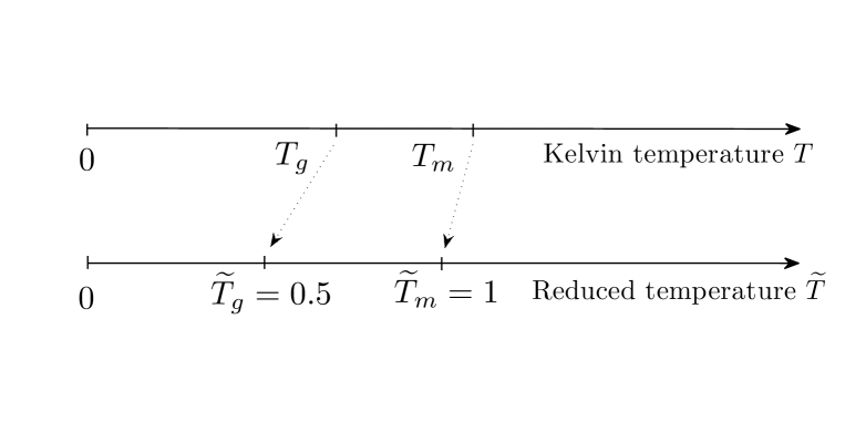
Figure 1: Demonstration of the transformation of the absolute temperature scale $T$ into the reduced temperature scale $\widetilde{T}$, which is system-independent and characterized by fixed values of the melting temperature $\widetilde{T}_{m}=1$ and the glass-transition temperature $\widetilde{T}_{g}=0.5$. Simple realization of the transition can be done by means of relation (2).

It should be pointed out that the temperatures $T=0$ K, $T_{g}$ and $T_{m}$ in relation (2) correspond to the same isobar. Relation (2) transforms the ($p,T$) phase diagram within the range $0\leq T\leq T_{m}$ to the ($p,\widetilde{T}$) phase diagram unified for all systems, where the glass transition line and the melting line are parallel to the ordinate, $p$-axis, and intersect the abscissa at $\widetilde{T}_{g}$=0.5 and $\widetilde{T}_{m}=1$, respectively.

III Simulation details and computational methods

In this work, we consider two model systems – the Dzugutov (Dz) system Dzugutov_1992 ; Dzugutov_2002 and the binary Lennard-Jones (bLJ) mixture Rowlinson_1969 ; Toxvaerd_Pedersen_2009 . Both systems are known as the model glass-formers suitable to study the properties of glasses by means of molecular dynamics simulations Roth_PRB_2005 ; Kob_Andersen_1993 ; Hansen_McDonald_2006 ; Ryzhov . In this work, the glassy samples were generated by fast quench of equilibrated fluids at the fixed pressure $p$. The corresponding pathways are shown on the phase diagrams in Fig. 2. Consideration of the ($p,T$)-points of the phase diagrams with high values of the pressure $p$ allows us to deal with such conditions at which the structural ordering in the glassy systems proceeds over time-scales available for simulations even at temperatures below $T_{g}$ (Refs. Mokshin/Barrat_PRE_2008 ; Mokshin/Barrat_PRE_2010 ). Thereby, the value of the pressure $p$ was chosen so that a clearly-detected nucleation event was observable over the simulation time scale. Hence, the simulations with the generated glassy samples were performed in the $NpT$-ensemble; $N$ is the number of particles. The constant temperature and pressure conditions are ensured by using the Nosé-Hoover thermostat and barostat. For each ($p,T$)-point, more than fifty independent samples were generated, the data of which were used in a statistical treatment. For a single simulation run, $N=6\,912$ particles were enclosed in a cubic cell with periodic boundary conditions. Note that the terms $\varepsilon$ and $\sigma$ define the units of energy and length, respectively. Time, pressure, and temperature units are measured in $\tau_{0}=\sigma\sqrt{m/\varepsilon}$, $\varepsilon/\sigma^{3}$, and $\varepsilon/k_{B}$, respectively.

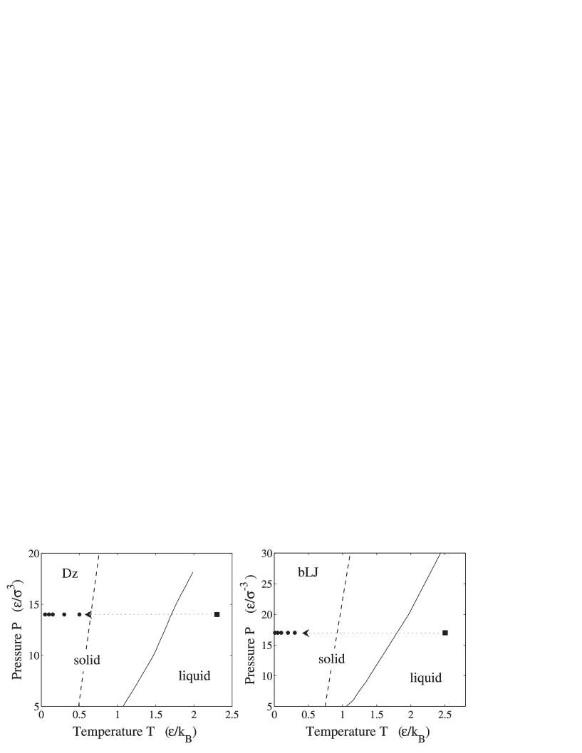
Figure 2: Pressure-temperature phase diagram for the Dz-system (left panel) and for the bLJ-system (right panel). The full curves denote the boundary between liquid and solid phases; the curve for the Dzugutov system is reproduced from data of Fig. 4 in Ref. Roth_PRB_2005 . The dashed curves mark the boundary between the supercooled liquid and the amorphous solid, when liquid is cooled during isobaric simulations with the rate $dT/dt=0.001$ $\varepsilon/(k_{B}\tau_{0})$. The full squares indicate the equilibrium liquid states, which were used as starting points to generate glassy samples. Pathways related with preparation of the glassy samples are schematically shown by dotted arrows; and the full circles denote the ($p,T$)-points, at which the transition into ordered states was tracked.

The Dzugutov system. – In case of the Dzugutov system, all particles are identical and interacting via a short-ranged pair potential

$$\frac{U^{Dz}(r^{*})}{\varepsilon} = A({r^{*}}^{-m}-B)\exp\left(\frac{c}{r^{*}-a}\right)\Theta(a-r^{*})$$ (4)

$$+ B\exp\left(\frac{d}{r^{*}-b}\right)\Theta(b-r^{*}),$$

$$\hskip 8.5359ptr^{*}=\frac{r_{ij}}{\sigma},$$

where $\Theta(\ldots)$ is the Heaviside step function, the values of parameters $A=5.82$, $B=1.28$, $m=16$, $a=1.87$, $b=1.94$, $c=1.1$ are chosen as suggested originally in Ref. Dzugutov_1992 . The simulations were performed for the system along the isobaric line with the pressure $p=14\,\varepsilon/\sigma^{3}$ at the temperatures $T=0.05$, $0.1$, $0.15$, $0.3$ and $0.5\,\varepsilon/k_{B}$ below $T_{g}\simeq 0.65\,\varepsilon/k_{B}$. For the isobar, the melting temperature is $T_{m}\simeq 1.51\,\varepsilon/k_{B}$, that yields the temperature ratio $T_{g}/T_{m}\simeq 0.43$.

The binary Lennard-Jones mixture. – The semi-empirical (incomplete) Lorentz-Berthelot mixing rules Rowlinson_1969 ; Toxvaerd_Pedersen_2009 ,

$$\sigma_{BB} = 0.8\sigma_{AA},$$

$$\sigma_{AB} = \frac{\sigma_{AA}+\sigma_{BB}}{2},$$

$$\varepsilon_{BB} = 0.5\varepsilon_{AA},$$

$$\varepsilon_{AB} = \varepsilon_{AA}+\varepsilon_{BB},$$

were utilized at the simulations of the binary Lennard-Jones system $A_{80}B_{20}$ with the potential

$$\frac{U_{\alpha\beta}^{bLJ}(r_{ij})}{\varepsilon_{\alpha\beta}}=4\left[\left(\frac{\sigma_{\alpha\beta}}{r_{ij}}\right)^{12}-\left(\frac{\sigma_{\alpha\beta}}{r_{ij}}\right)^{6}\right],$$ (5)

where $\alpha$, $\beta\in\{A,\,B\}$, the labels $A$ and $B$ denote the type of particles, $r_{ij}$ is the distance between the centers of particles $i$ and $j$. Note that we take $\varepsilon=\varepsilon_{AA}$, $\sigma=\sigma_{AA}$, and the mass of a particle is $m=m_{A}=m_{B}=1$. For the bLJ system, we consider the isobar with the pressure $p=17\,\varepsilon/\sigma^{3}$ at the temperatures $T=0.01$, $0.05$, $0.1$, $0.2$ and $0.3\,\varepsilon/k_{B}$, that are lower than the transition temperature $T_{g}\simeq 0.92\,\varepsilon/k_{B}$. The isobar contains the melting point with $T_{m}\simeq 1.65\,\varepsilon/k_{B}$. Therefore, the temperature ratio is estimated as $T_{g}/T_{m}\simeq 0.56$.

Cluster analysis. – The local domains of a crystalline symmetry are examined by means of the cluster analysis Auer_Frenkel_2004 ; Mokshin_Barrat_2009 , introduced originally by Wolde-Frenkel Wolde-Frenkel . The consideration of the local environment around each particle is performed by means of $13$-dimensional complex vector with the components Steinhardt_Nelson_1983

$$q_{6m}(i)=\frac{1}{N_{b}(i)}\sum_{j=1}^{N_{b}(i)}Y_{6m}(\theta_{ij},\varphi_{ij}).$$ (6)

Here, $Y_{6m}(\theta_{ij},\varphi_{ij})$ are spherical harmonics, $N_{b}(i)$ is the number of neighbors for $i$ particle, $\theta_{ij}$ and $\varphi_{ij}$ are polar and azimuthal angles, which characterize the radius-vector $\vec{r}_{ij}$. Then, the local order for each $i$ particle can be numerically evaluated by means of the parameter Steinhardt_Nelson_1983

$$q_{6}(i)=\left(\frac{4\pi}{13}\sum_{m=-6}^{6}|q_{6m}(i)|^{2}\right)^{1/2},$$ (7)

whereas degree of the orientational order can be estimated by means of the global orientational order parameter $Q_{6}$ defined as an average of $q_{6}(i)$ over all $N$ particles Steinhardt_Nelson_1983 :

$$Q_{6}=\frac{1}{N}\sum_{i=1}^{N}q_{6}(i).$$ (8)

For a fully disordered system the parameter $q_{6}(i)$ is close to zero, while it grows with increasing structural ordering. For perfect fcc, bcc and hcp systems one has the largest possible values for the parameters Steinhardt_Nelson_1983 :

$$q_{6}(i)=Q_{6}\simeq 0.5745\ \ \ \ \ \mathrm{(fcc)},$$

$$q_{6}(i)=Q_{6}\simeq 0.5106\ \ \ \ \ \mathrm{(bcc)},$$

$$q_{6}(i)=Q_{6}\simeq 0.4848\ \ \ \ \ \mathrm{(hcp)}.$$

First, we define “neighbors” as all particles located within the first coordination, the radius of which is associated with position of the first minimum in the pair distribution function Mokshin/Barrat_PRE_2008 . Further, according to the Wolde-Frenkel scheme Wolde-Frenkel we specify the pair of neighboring particles ($i$ and $j$) as connected by a crystal-like bond if the following condition is fulfilled:

$$0.5<\left|\sum_{m=-6}^{6}\tilde{q}_{6m}(i)\tilde{q}_{6m}^{*}(j)\right|\leq 1,$$ (9)

where

$$\tilde{q}_{6m}(i)=\frac{{q}_{6m}(i)}{\left[\displaystyle{\sum_{m=-6}^{6}}|{q}_{6m}(i)|^{2}\right]^{1/2}}.$$ (10)

Condition (9) allows one to distinguish the particles correlated into an ordered structure Wolde-Frenkel . Finally, particle $i$ is identified as included into a crystalline structure if it has four and more crystal-like bonds. The last condition is applied to exclude from consideration the structures with a negligible number of bonds per particle, which occurs even in equilibrium liquid phase Mokshin/Barrat_PRE_2010 . By means of this routine, the particles involved into the crystalline domains are detected.

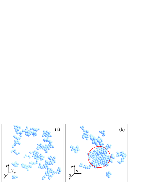
Figure 3: (Color online) Snapshots of the Dz-system at $T=0.5\,\varepsilon/k_{B}$ and at different times, for which the particles recognized as belonging to the crystalline phase are shown only. (a) System at the transient nucleation period; $t=100\,\tau_{0}$. There are no nuclei capable to grow, and their sizes are smaller than the critical size $n_{c}$. (b) System at the time $t=250\,\tau_{0}$, when the first critically-sized nucleus emerges; $n_{c}\simeq 105$ partilces. The critically-sized nucleus is marked by red circle.

Figure 3 demonstrates, as an example, the crystalline clusters emerging in the glassy Dz-system at $T=0.5\,\varepsilon/k_{B}$ over the transient nucleation regime, where no nuclei capable to grow are detected [Fig.  3(a)], and at the time $t=250\,\tau_{0}$, when the first nucleus of the critical size appears [Fig.  3(b)].

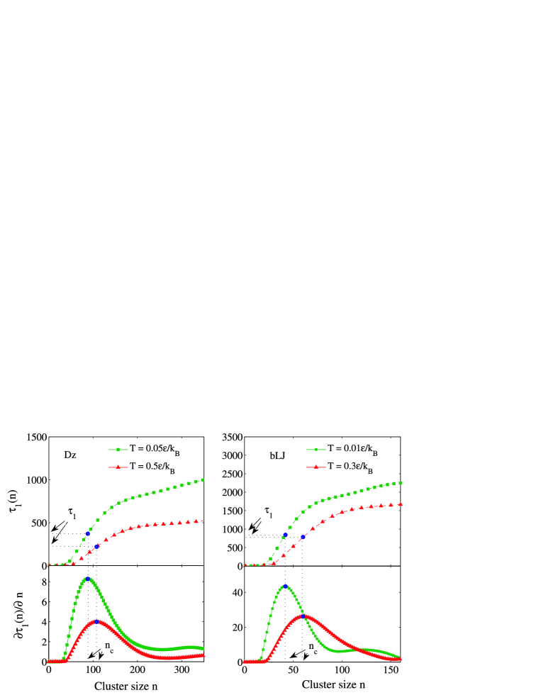
Figure 4: (Color online) Mean-first-passage-time distributions $\tau_{1}(n)$ and its first derivatives $\partial\tau_{1}(n)/\partial n$ defined from simulation data for the Dz-system and the bLJ-system at different temperatures.

Statistical treatment of the cluster analysis results. – The growth trajectories of the crystalline nuclei, $n_{\alpha i}(t)$, extracted from the different simulation runs are treated within the mean-first-passage-time method Mokshin/Galimzyanov_JCP_2014 ; Mokshin_Galimzyanov_JPCB_2012 . Here, $n$ defines number of the particles involved in the nucleus at the time $t$, the mark $\alpha$ denotes the index of simulation run, whereas the order number of the nucleation event $i$ indicates that the $i$th nucleus of the size $n$ appears at the time $t$ during the $\alpha$th simulation run. On the basis of the extracted trajectories $n_{\alpha i}(t)$, the mean-first-passage-time distributions $\tau_{i}(n)$ are evaluated for each $i$th-order nucleus (for details, see Ref. Mokshin_Galimzyanov_JPCB_2012 ). Further, the critical size $n_{c}$ and the average waiting time for the $i$th-order nucleus, $\tau_{i}$, $i=1,\,2,\,\ldots$, are defined from the analysis of the distributions $\tau_{i}(n)$ and of the first derivatives $\partial\tau_{i}(n)/\partial n$, according to the scheme suggested in Ref. Mokshin/Galimzyanov_JCP_2014 . In this work, we focus on the characteristics for the largest nucleus – i.e. on its critical size $n_{c}$ and average waiting time $\tau_{1}$.

As an example, we show in Fig. 4 the mean-first-passage-time distribution $\tau_{1}(n)$ and its first derivative $\partial\tau_{1}(n)/\partial n$ computed for both the systems. As can be seen, the distributions $\tau_{1}(n)$ are characterized by three regimes. The first regime, for which small values of $n$ correspond to $\tau_{1}(n)$ with zero value, is associated with pre-nucleation. Here, the nuclei with different sizes (albeit, small sizes) appear with equal probability. The second regime, in which the distribution $\tau_{1}(n)$ has the pronounced non-zero slope, contains information about a nucleation event. Namely, detected from the first derivative $\partial\tau_{1}(n)/\partial n$ location of an inflection point in the distribution $\tau_{1}(n)$ for the regime defines the critical size $n_{c}$, whereas $\tau_{1}(n_{c})\equiv\tau_{1}$ is directly associated with the average waiting time of the first critically-sized nucleus Mokshin/Galimzyanov_JCP_2014 . Finally, the third regime, where the slope of $\tau_{1}(n)$ decreases, corresponds to growth of the nucleus. Note that such shape of the mean-first-passage-time distribution is typical for an activated process. The absence of the pronounced plateau in $\tau_{1}(n)$ for the third regime indicates that the nuclei growth proceeds over a time-scale comparable the nucleation time $\tau_{1}$ (Ref. Mokshin_Galimzyanov_JPCB_2012 ).

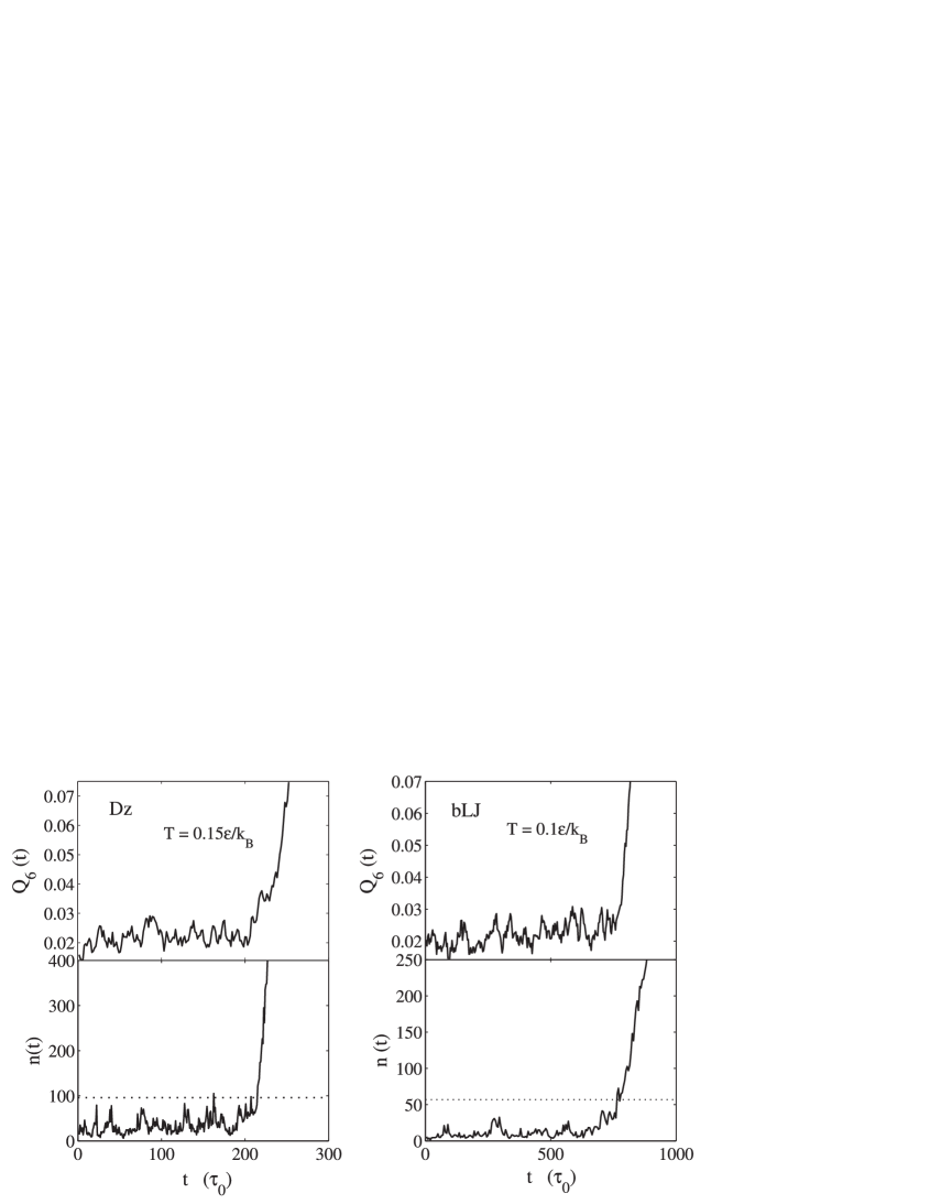
Figure 5: Trajectories of the global orientational order parameter $Q_{6}(t)$ and of the largest crystalline nucleus size $n(t)$ defined from a single simulation run for the Dz-system (left panel) and the bLJ-system (right panel). The dotted horizonal lines on the plots for $n(t)$ correspond to the critical sizes $n_{c}$ defined from the statical analysis within the mean-first-passage-time method.

IV Discussion of results

We start from evaluation of some properties of the nascent ordered structures, that can help to elucidate the mechanism of the ordering. Figure 5 shows the time-dependent order parameters – the global orientational order parameter, $Q_{6}(t)$, and the size of the largest cluster, $n(t)$, – evaluated on the basis of the simulation data. In initial stages, the parameters $Q_{6}(t)$ and $n(t)$ fluctuate around their starting values. After an incubation time, both the parameters start to growth rapidly. Such evolution of the order parameters indicates on activated character of the transition Hanggi_RMP_1990 . The nucleation event is clear detectable on a particular trajectory $n(t)$, where it is associated with the start of sharp grow of $n(t)$. While rough estimates for the nucleation time-scale $\tau_{1}$ and for the critical size $n_{c}$ can be done even from the particular trajectories $n(t)$ [see Fig. 5], the averaged values for both the quantities can be computed directly by means of the statistical method presented in Sec. III.

Further, cluster analysis reveals that the nuclei of the critical size are localized. As contrasted to Ref. Trudu/Parinello , no ramified structures were detected even at very deep supercooling. For quantitative characterization, the asphericity parameter $S_{0}$ was computed according to

$$S_{0}=\left\langle\frac{(I_{xx}-I_{yy})^{2}+(I_{xx}-I_{zz})^{2}+(I_{yy}-I_{zz})^{2}}{2(I_{xx}+I_{yy}+I_{zz})^{2}}\right\rangle,$$ (11)

where

$$I_{\alpha\beta}=\sum_{i=1}^{n_{c}}m(r_{i}^{2}\delta_{\alpha\beta}-r_{i\alpha}r_{i\beta})$$ (12)

defines the components of the moment of inertia tensor associated with a critically-sized nucleus; the brackets $\langle\ldots\rangle$ mean the statistical average over results of the different simulation runs. The parameter $S_{0}$ approximates the unity, $S_{0}\rightarrow 1$, for an elongated and ramified cluster, and one has $S_{0}\rightarrow 0$ for a cluster, the envelope of which is of spherical shape. For both the systems (Dz and bLJ), we find that the asphericity parameter is $S_{0}\simeq 10^{-3}$, and the size of the critical nucleus remains finite. This is evidence that the transition into an ordered phase is initiated rather through nucleation mechanism, and that is in agreement with findings of Refs. Saika_Voivod_JCP_2007 ; Bartell_JCP_2007 . For the Dz-system, our estimations reveal that the critical size changes from $n_{c}=108\pm 5$ to $88\pm 6$ particles with the temperature decrease (increase of supercooling) from $T=0.5\,\varepsilon/k_{B}$ to $0.05\,\varepsilon/k_{B}$. For the bLJ-system, we find that the critical size decreases from $n_{c}=59\pm 4$ to $42\pm 3$ particles with the temperature decrease within the range $0.3\,\varepsilon/k_{B}\geq T\geq 0.01\,\varepsilon/k_{B}$.

Figure 6 shows the values of the average waiting time of the first nucleus of the critical size, $\tau_{1}$, estimated from simulation data for the Dz-system and the bLJ-system at the different temperatures. We note that the deep levels of supercooling are considered for both the systems corresponding to the temperatures much below $T_{g}$. The particle mobility diminishing with supercooling results in the growth of $\tau_{1}$ with the temperature decrease. The finite values of $\tau_{1}$ comparable with the duration of numerical experiment may seem surprising for a glassy system. Actually, the microscopic kinetics of a glass changes with moving over phase diagram for the range of high pressures Tanguy_2012 . Namely, at high pressures the structural relaxation as well as the transition of glassy system into a state with the lower free energy proceeds over shorter time scales Saika_Voivod_PRL_2011 ; Khusnutdinoff/Mokshin_PhA_2012 ; Khusnutdinoff/Mokshin_JNCS_2011 . Therefore, the reduction of the values of $\tau_{1}$ is admissible for the range of phase diagrams.

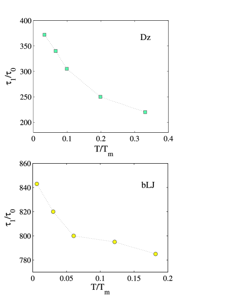
Figure 6: (Color online) Average waiting time of the first critically-sized nucleus $\tau_{1}$ (in units of $\tau_{0}$) versus reduced temperature for the Dz-system ($T_{g}/T_{m}=0.43$) and for the bLJ-system ($T_{g}/T_{m}=0.56$). The spanned thermodynamic ranges correspond to deep levels of supercooling with the temperatures below $T_{g}$.

Table 1: The melting temperature $T_{m}$, the ratio $T_{g}/T_{m}$, the waiting time for the first critically-sized nucleus $\tau_{1}^{g}$ at the transition temperature $T_{g}$, the exponent $\gamma$ estimated from Eq. (13), the parameters $K_{1}$ and $K_{2}$ evaluated by Eq. (3b) for several systems.

System	$T_{m}$	$T_{g}/T_{m}$	$\tau_{1}^{g}$	$\gamma$	$K_{1}$	$K_{2}$
Dz (at $p=14\varepsilon/\sigma^{3}$)	$1.51\;\varepsilon/k_{B}$	$0.43$	$211\,\tau_{0}$	$0.27$	$0.553$	$-0.053$
bLJ (at $p=17\varepsilon/\sigma^{3}$)	$1.65\;\varepsilon/k_{B}$	$0.56$	$760\,\tau_{0}$	$0.025$	$0.427$	$0.073$
Li2O$\cdot 2$SiO2	$1286$ K	$0.56$	$1869$ sec	$70$	$0.424$	$0.076$
Na2O$\cdot 2$CaO$\cdot 3$SiO2	$1549$ K	$0.53$	$5150$ sec	$50$	$0.466$	$0.034$
K2O$\cdot$TiO${}_{2}\cdot 3$GeO2	$1308$ K	$0.63$	$990$ sec	$30$	$0.281$	$0.219$

Although the quantity $\tau_{1}$ for both the systems demonstrates similar temperature dependence, it is difficult to say something about quantitative correspondence to the general nucleation trends. Is such temperature dependence of the nucleation waiting time, $\tau_{1}(T)$, is typical for the considered thermodynamic range or not? One of the possible ways to clarify this is to bring the extracted values of the nucleation waiting time $\tau_{1}(T)$ into a unified scaled dependence. To construct scaling relation, we propose to use the reduced temperature $\widetilde{T}$ defined by relation (2), in which the values of the glass transition temperature and the melting temperature are fixed for all systems. Then, the simplest nonlinear $\widetilde{T}$-dependence of $\tau_{1}$ can be chosen in the form:

$$\tau_{1}=\tau_{1}^{g}\left(\frac{\widetilde{T}_{g}}{\widetilde{T}}\right)^{\gamma},$$ (13)

where $\tau_{1}^{g}$ is the average waiting time for the first critically-sized nucleus at the state with the temperature $T_{g}$ (we remind that $\widetilde{T}_{g}=0.5$). The dimensionless parameter $\gamma>0$ characterizes ability of the system at the considered ($p,T$)-state to retain structural disorder. In particular, the exponent $\gamma$ takes high values for the system with good glass-forming properties, and must be characterized by small values for the fast crystallizing systems. Since the nucleation waiting time $\tau_{1}$ varies with pressure, then the exponent $\gamma$ should be dependent on the pressure, at which a supercooled liquid evolves. Namely, the exponent $\gamma$ is decreasing function of the pressure $p$ for the systems, in which the nucleation time scale decreases with pressure. The Dz and bLJ systems correspond to the case.

To verify validity of relation (13), we place the rescaled data for the average waiting time $\tau_{1}$ for the Dz and bLJ systems vs. the reduced temperature $\widetilde{T}$ on the common Fig. 7. For clarity, the axis of ordinates is presented on a logarithmic scale, where the fitting parameter $\gamma$ corrects the slope in accordance with the master-curve

$$\left(\frac{\tau_{1}}{\tau_{1}^{g}}\right)=\frac{\widetilde{T}_{g}}{\widetilde{T}},$$ (14)

which appears from (13) at the exponent $\gamma=1$. The reduced temperature $\widetilde{T}$ in Eq. (13) guarantees that the temperature points spread over the abscissa in the same manner for all the considered systems, whereas the dimensionless parameter $\gamma$ forces all the ordinate points to collapse onto the master-curve (14). Since our simulation results for the Dz and bLJ systems cover the temperature range $T<T_{g}$ and we did not estimate the nucleation time $\tau_{1}$ at the transition temperature $T_{g}$, then the term $\tau_{1}^{g}$ was taken as a fitting parameter. Namely, its values were found by extrapolation of the data for $\tau_{1}$ to the temperature point $\widetilde{T}_{g}=0.5$, where the function $(1/\gamma)\log(\tau_{1}/\tau_{1}^{g})$ must be equal to zero (see Fig. 7). Numerical values of $\tau_{1}^{g}$ are given in Tab. 1. As can be seen from Fig. 7, all the data obtained on the basis of molecular dynamics simulations follow the unified master-curve. Moreover, in contrast to the case of the Kelvin temperature scale, values of the melting temperature $\widetilde{T}_{m}$ and of the transition temperature $\widetilde{T_{g}}$ are not dependent on pressure. Therefore, the results shown on Fig. 7 can be supplemented by the data for any supercooled liquid at arbitrary value of the pressure $p$.

Moreover, it is attractive to extend the study and to verify the scaling law (13) with the experimental data. While the direct experimental measurements of $\tau_{1}$ are difficult Shneidman , we suggest the next routine for the approximative estimation of $\tau_{1}$, which can be realized with the experimentally measurable quantities – the steady-state nucleation rate $J_{s}$ and the induction time $\tau_{ind}$. According to Kashchiev Kashchiev_1969 ; Kashchiev_Nucleation_2000 , the number density of the supercritical nuclei in the system, $i_{V}$, evolves with time as

$$\frac{i_{V}(t)}{J_{st}\tau_{ind}} = \frac{t}{\tau_{ind}}-1$$

$$- \frac{12}{\pi^{2}}\sum_{m=1}^{\infty}\frac{(-1)^{m}}{m^{2}}\exp\left(-\frac{m^{2}\pi^{2}t}{6\tau_{ind}}\right).$$

For the time $t=\tau_{1}$ one has $i_{V}(\tau_{1})=1/V$, and Eq. (IV) takes the form:

$$\frac{1}{J_{st}V} = \tau_{1}-\tau_{ind}$$

$$+ \frac{12\tau_{ind}}{\pi^{2}}\sum_{m=1}^{\infty}\frac{(-1)^{m}}{m^{2}}\exp\left(-\frac{m^{2}\pi^{2}\tau_{1}}{6\tau_{ind}}\right).$$

Further, Eq. (IV) was numerically solved with the experimental $J_{s}$ and $\tau_{ind}$ for Li₂O$\cdot 2$SiO₂ reported in Ref. Fokin/Yuritsyn/Zanotto_review , for Na₂O$\cdot 2$CaO$\cdot 3$SiO₂ presented in Ref. Fokin/Zanotto_JNCS_2000 , and for K₂O$\cdot$TiO${}_{2}\cdot 3$GeO₂ given in Ref. Grujic_2009 . The extracted rescaled values of the average waiting time $\tau_{1}$ are also presented in Fig. 7. As can be seen from Fig. 7, “experimental” data for $\tau_{1}$ provide the $T$-dependence, which is in agreement with scaling relation (13) as well as with the simulation results for the bLJ-system and the Dz-system.

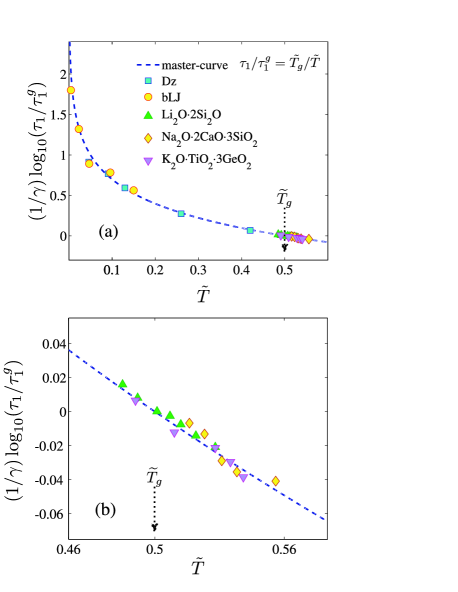
Figure 7: (Color online) (a) Scaled waiting time for the first critically-sized nucleus $(1/\gamma)\log_{10}(\tau_{1}/\tau_{1}^{g})$ is plotted as a function of the reduced temperature $\widetilde{T}$. Here, $\widetilde{T}_{g}=0.5$ is the scaled transition temperature (marked by arrow), $\tau_{1}^{g}$ is the waiting time at the transition temperature ${T}_{g}$, and $\gamma$ is the fitting parameter. (b) The same but for the temperature range $0.46\leq\widetilde{T}\leq 0.58$. Values of the parameters $\tau_{1}^{g}$ and $\gamma$ are given in Tab. 1. Consistency of the data to the master-curve, which set the temperature-dependence $\widetilde{T}_{g}/\widetilde{T}$, provides support to the validity of scaling relation (13).

Analysis of the reduced temperature scale $\widetilde{T}$ for the systems reveals that the quadratic contribution in equation for $\widetilde{T}$ [see Eq. (2)] can be insignificant as for the Dz-system and for Na₂O$\cdot 2$CaO$\cdot 3$SiO₂, where the ratio $T_{g}/T_{m}$ is equal to $0.43$ and $0.53$, respectively (see Tab. 1). With away from value $0.5$ for the ratio $T_{g}/T_{m}$, weight of the quadratic contribution, $K_{2}$, increases. The values of the parameters $K_{1}$ and $K_{2}$ are comparable for K₂O$\cdot$TiO${}_{2}\cdot 3$GeO₂ characterized by the ratio $T_{g}/T_{m}=0.63$. To our knowledge, the highest value of the ratio $T_{g}/T_{m}$ appears for Na₂O$\cdot$Al₂O${}_{3}\cdot 6$SiO₂ and is equal to $0.78$ (Ref. Fokin/Yuritsyn/Zanotto_review ).

The values of the exponent $\gamma$ differ for the considered systems by four orders of magnitude, and an order of magnitude between the Dz-system and the bLJ-system (see Tab. 1). The large scatter in the values of $\gamma$ is due to the change of the waiting nucleation time $\tau_{1}$ within the temperature range differs essentially for the systems. One can demonstrate this with the results for the Dz and bLJ systems shown on Fig. 6. Within the temperature range $0.025\leq T/T_{m}\leq 0.2$ the time scale $\tau_{1}$ is changed by the factor $0.625$ for the Dz-system, whereas it changes by the factor $0.96$ for the bLJ-system. For the systems with complicated structural units (i.e. for silicate glasses) the change is much more pronounced Fokin/Yuritsyn/Zanotto_review . The case with the smaller change in the temperature dependence of $\tau_{1}$ will corresponds to the smaller values of the exponent $\gamma$ in scaling relation (13).

Although the scaling law (13) is suggested rather as an empirical result, its qualitative justification can also be done. At the temperatures comparable with and lower than the glass transition temperature $T_{g}$, the local structural rearrangements responsible for the nucleation are driven rather by kinetic aspects associated with the viscosity than by thermodynamic contribution. Therefore, it is reasonable for the range of high supercooling to expect the existence of correlation between the waiting time for nucleation $\tau_{1}(T)$ and the structural relaxation time $\tau_{\alpha}(T)\sim\eta(T)$, and, thereby, between the time $\tau_{1}(T)$ and the viscosity $\eta(T)$:

$$\tau_{1}(T)\sim\eta(T).$$ (17)

Hence, the Vogel-Fulcher-Tammann equation provides the most popular viscosity model (this equation is also known as the Williams-Landel-Ferry model Seeton ; Allan_PNAS ):

$$\log_{10}{\eta}(T)=\log_{10}{\eta}_{\infty}+\frac{A}{T-T_{c}},$$ (18)

where $T_{c}$ is the critical temperature of this model. Another equation for viscosity similar to VFT-model is provided by the mode-coupling theory Angell_Leningrad_1989 ; Gotze_book_2009 :

$$\eta(T)=\frac{{\eta}_{\infty}}{(T-T_{MCT})^{\gamma_{m}}},$$ (19)

where $T_{MCT}$ is the (critical) mode-coupling temperature. The parameters ${\eta}_{\infty}$, $A$ and $\gamma_{m}$ take positive values and are obtained by fitting Eqs. (18), (19) to experimentally measured viscosity data Allan_PNAS . Both the models predict a divergence of the viscosity $\eta(T)$ when $T\rightarrow T_{c}$ (and $T\rightarrow T_{MCT}$). Moreover, both the models are able to reproduce $\eta(T)$ for the supercooled liquid phase, i.e. $T>T_{c}$ (and $T>T_{MCT}$), and are not applicable for the temperature range below $T_{c}$ (below $T_{MCT}$) because of a divergence in the temperature dependencies. On the other hand, for a high-viscosity regime corresponding to the temperatures $T\leq T_{g}$, the experimentally measured temperature-dependence of the viscosity $\eta(T)$ is reproducible by the Arrhenius law (see, for example, Fig. 6 in Ref. Bottinga ), which is generalized by the Avramov-Milchev equation Avramov/Milchev_1988 ; Allan_PNAS :

$$\log_{10}\eta(T)=\log_{10}\eta_{\infty}+\left(\frac{\mathcal{A}}{T}\right)^{\alpha^{\prime}}$$ (20)

or

$$\log_{10}\left[\frac{\eta(T)}{\eta_{\infty}}\right]=\left(\frac{T}{\mathcal{A}}\right)^{-\alpha^{\prime}},$$ (21)

where $A$ and $\alpha^{\prime}$ are positive.

On the other hand, let us now reconsider scaling relation (13), which can be rewritten in the form

$$\frac{\tau_{1}}{\tau_{1}^{g}}=\left(2\widetilde{T}\right)^{-\gamma},$$ (22)

since $\widetilde{T}_{g}=0.5$. After substitution of Eq. (2) into relation (22) and using the expansion

$$\ln(x+1)=\sum_{n=1}^{\infty}\frac{(-1)^{n-1}x^{n}}{n},\hskip 28.45274pt-1<x<1,$$ (23)

we obtain for the temperature range $0<T<T_{m}$ the following equation:

$$\log_{10}\left[\frac{\tau_{1}(T)}{\tau_{1}^{g}}\right] = \frac{1}{\ln{10}}\sum_{n=1}^{\infty}\frac{(-1)^{n-1}}{n}$$

$$\times\left(\frac{T}{T_{g}}\right)^{-\gamma n}\left[\left\{2K_{1}\left(1-\frac{T}{T_{g}}\right)+\frac{T}{T_{g}}\right\}^{-\gamma}-\left(\frac{T}{T_{g}}\right)^{\gamma}\right]^{n},$$

where the parameter $K_{1}$ is defined by Eq. (3b). Assuming that proportionality in Eq. (17) holds, one can compare r.h.s. of Eqs. (21) and (IV). A simple analysis reveals that Eq. (IV) is able to approximate the power-law dependence of Eq. (21) and generalizes the temperature dependence for the viscosity given by the Avramov-Milchev equation. Thereby, the scaling relation (13) and the viscosity model with Eq. (21) can be considered as consistent.

Moreover, the fragility of a system can be estimated by means of the index $m$ defined as Angell_1995

$$m=\left.\frac{\partial\log_{10}(\eta)}{\partial(T_{g}/T)}\right|_{T=T_{g}}.$$ (25)

Then, from Eqs. (17), (22) and (25) we obtain the following relation

$$m\sim\left.\frac{\partial\log_{10}(\tau_{1})}{\partial(T_{g}/T)}\right|_{T=T_{g}}\sim 2\gamma(1-K_{1}),$$ (26)

which after substitution of Eq. (3b) can be rewritten as

$$m\propto 2\gamma\left[\frac{\displaystyle 0.5-\frac{T_{g}}{T_{m}}+\left(\frac{T_{g}}{T_{m}}\right)^{2}}{\displaystyle 1-\frac{T_{g}}{T_{m}}}\right].$$ (27)

Here the contribution in square brackets is positive for the range $0\leq(T_{g}/T_{m})\leq 1$. Last two relations indicates that the exponent $\gamma$ and the index $m$ are correlated terms, whereas $\gamma$ can provide an estimate of fragility.

V Conclusion

The mechanism of the structural ordering in the supercooled melts at extremely deep level of supercooling is one of the most debated issues in the consideration of the crystallization kinetics van_Megen_Nature_1993 ; Cavagna_2003 ; Cavagna_2007 . Let us mention some viewpoints in this regard. The mean-field theories, starting from the gradient theory of Cahn-Hilliard, provide indications that the structural ordering at a deep level of metastability can proceed through the spinodal decomposition Cahn/Hilliard_JCP_1959 . Interestingly, Trudu et al. for the freezing bulk Lennard-Jones system found a spatially diffuse and collective phenomenon of nucleation at deep supercooling. Authors treated such features as indirect signatures of a mean-field spinodal Trudu/Parinello . This was later criticized by Bartell and Wu Bartell_JCP_2007 . According to experimental Pan_2006 and other simulation Bagchi_2007 ; Saika_Voivod_JCP_2007 studies, the size of the critical embryo remains finite with decrease of the temperature of the supercooled liquid, in contrast to the mean-field theory predictions for a spinodal. Moreover, results of Ref. Sanz_PRL_2011 reveal that crystallization in hard sphere glasses proceeds due to “a chaotic sequence of random micronucleation events, correlated in space by emergent dynamic heterogeneity”, and agree with findings of Bartell-Wu Bartell_JCP_2007 . In view of this, it remains still desirable to examine the mechanisms of the structural ordering in glasses within the new experimental/simulation results.

In the present work, two model glassy systems with different interparticle interaction – the single-component Dzugutov system and the binary Lennard-Jones system – are simulated with the aim to study the structural ordering at deep supercooling. Remarkably, the simulation study covers a wide temperature range: from the temperatures comparable with $T_{g}$ to the temperatures corresponding to very deep levels of supercooling $(T_{m}-T)/T_{m}\simeq 0.97$. By means of cluster analysis, we show that the structural ordering even at deep supercooling proceeds through the formation of the localized crystalline domains, where the size of the critical embryo still remains finite. This supports the nucleation scenario of crystallization in the glassy systems, and is in agreement with the recent findings of Saika-Voivod et al.  Saika_Voivod_PRL_2011 ; Saika_Voivod_JCP_2007 and Sanz et al. Sanz_PRL_2011 .

The average nucleation time is the quantity of main interest in the characterization of the initial stages in the nucleation kinetics. Here, it is estimated on the basis of the molecular dynamics simulation data (for the two model glassy systems) and from the available experimental data for the several glasses within the Kashchiev’s approximative equation. Our results show that, with the decrease of the temperature, the nucleation time $\tau_{1}$ increases but still remains finite. Further, we find that the nucleation time $\tau_{1}$ plotted as a function of the proposed reduced temperature follows the power-law dependence, unified for all the considered systems. The correlation between the proposed reduced temperature dependence for $\tau_{1}$ and the viscosity models for the amorphous solids supports the conclusion about the kinetic character of the initiation of the structural ordering in glasses, where the inherent glassy microscopic dynamics is predominating over thermodynamic aspects.

Results of this study extend the idea of a unified description of the nucleation kinetics using scaling relations, which was originally applied to the analysis of the droplet nucleation rate data for the vapor-to-liquid transition (see Hale_1 and references to Hale_2 ). The later treatment indicates that the nucleation rate can be well described by the scaling function $\ln(p/p_{coex})/[T_{c}/T-1]^{3/2}$. In this study, we pursue a similar approach applied to crystallization and define such a variable, which might provide consistency in comparison of the crystal nucleation time data for different systems. Our realization differs from the scalings of Ref. Diemand_2 ; Hale_1 ; it is based on the reduced temperature scale with the fixed control points: the temperature $\widetilde{T}=0$, the glass transition temperature $\widetilde{T}_{g}=0.5$ and the melting temperature $\widetilde{T}_{m}=1$ for a considered system. Using this approach we find a correspondence of the scaled nucleation times as extracted from simulation and experimental data for the various systems to a unified power-law dependence. Finally, we note that because of experimental difficulties in extraction of the quantitative information about the initial stages of the crystallization kinetics, few of the experimental studies cover the range of supercooling $(T_{m}-T)/T_{m}>0.6$ Fokin/Zanotto_2003 . In this regard, it could be desirable to verify the suggested scaling law with additional experimental studies, especially, for the glassy systems at deep supercooling.

- [1] J. Frenkel, Kinetic Theory of Liquids (Oxford University Press, London, 1946).
- [2] D. Turnbull, in: J.A. Prins (Ed.), Physics of Non-Crystalline Solids (North Holland Publishing Company, Amsterdam, 1965).
- [3] V.P. Skripov, Metastable Liquids (Wiley, New York, 1974).
- [4] K.F. Kelton, Solid State Phys. 45, 75 (1991).
- [5] P.G. Debenedetti, Metastable Liquids. Concepts and Principles (Princeton Univ. Press, Princeton, 1996).
- [6] D. Kashchiev, Nucleation: Basic Theory with Appplications (Butterworth-Heinemann, Oxford, 2000).
- [7] V.I. Kalikmanov, Nucleation Theory, Lecture Notes in Physics vol. 860(Springer, New York, 2012).
- [8] I. Saika-Voivod, R.K. Bowles, and P.H. Poole, Phys. Rev. Lett. 103, 225701 (2009).
- [9] A.V. Mokshin, J.-L. Barrat, Phys. Rev. E 82, 021505 (2010).
- [10] A.V. Mokshin, J.-L. Barrat, Phys. Rev. E 77, 021505 (2008).
- [11] A. Kerrache, N. Mousseau and L.J. Lewis, Phys. Rev. B 83, 134122 (2011).
- [12] A. Kerrache, N. Mousseau and L.J. Lewis, Phys. Rev. B 84, 014110 (2011).
- [13] D.M. Heyes, E.R. Smith, D. Dini, H.A. Spikes and T.A. Zaki, J. Chem. Phys. 136, 134705 (2012).
- [14] A.V. Mokshin, B.N. Galimzyanov and J.-L. Barrat, Phys. Rev. E 87, 062307 (2013).
- [15] B.R. Durschang, G. Carl, C. Rüssel and I. Gutzow, Berichte der Bunsengesellschaft für physikalische Chemie 100, 1456 (1996).
- [16] I. Gutzow, C. Rüssel, and B. Durschang, J. Mater. Sci. 32, 5405 (1997).
- [17] P.F. Xing, Y.X. Zhuang, W.H. Wang, L. Gerward and J.Z. Jiang, J. Appl. Phys. 91, 4956 (2002).
- [18] C. Yang et. al J. Phys.: Condens. Matter 20, 015201 (2008).
- [19] K. Niss et. al, J. Chem. Phys. 129, 194513 (2008).
- [20] B. Mantisi, A. Tanguy, G. Kermouche, E. Barthel, Eur. Phys. J. B 85, 304 (2012).
- [21] E.D. Zanotto, V.M. Fokin, Phil. Trans. R Soc. Lond. A 361, 591 (2002).
- [22] A.M. Kalinina, V.N. Filipovich, V.M. Fokin, G.A. Sycheva, in: Proc. XIV Int. Cong. on Glass, New Delhi 1, 366 (1986).
- [23] R. Müller, E.D. Zanotto, V.M. Fokin, J. Non-Cryst. Solids 274, 208 (2000).
- [24] V.M. Fokin, E.D. Zanotto, J.W.P. Schmelzer, J. Non-Cryst. Solids 321, 52 (2003).
- [25] V.M. Fokin, E.D. Zanotto, N.S. Yuritsyn, J.W.P. Schmelzer, J. Non-Cryst. Solids 352, 2681 (2006).
- [26] P.F. James, in: M.H. Lewis (Ed.), Glasses and Glass-Ceramics (Chapman and Hall, London, 1989).
- [27] E.D. Zanotto, J. Non-Cryst. Solids 89, 361 (1987).
- [28] J. Deubener, J. Non-Cryst. Solids 274, 195 (2000).
- [29] S. V. Shevkunov, Colloid Journal 75, 444 (2013).
- [30] K. Binder and D. Stauffer, Adv. Phys. 25, 343 (1976).
- [31] B.N. Hale, Phys. Rev. A 33, 4156 (1986).
- [32] B.N. Hale, J. Chem. Phys. 122, 204509 (2005).
- [33] B.N. Hale and M. Thomason, Phys. Rev. Lett. 105, 046101 (2010).
- [34] J. Diemand, R. Angélil, K.K. Tanaka, and H. Tanaka, J. Chem. Phys. 139, 074309 (2013).
- [35] K.K. Tanaka, J. Diemand, R. Angélil, and H. Tanak, J. Chem. Phys. 140, 194310 (2014).
- [36] B.N. Hale, Lecture Notes in Physics 309, 323 (1988).
- [37] C.A. Angell, C.A. Scamehorn, D.J. List, and J. Kieffer, Proceedings of XV International Congress on Glass (Leningrad, 1989).
- [38] C.A. Angell, Science 267, 1924 (1995).
- [39] M. Dzugutov, Phys. Rev. A 46, R2984 (1992).
- [40] M. Dzugutov, S.I. Simdyankin, F.H.M. Zetterling, Phys. Rev. Lett. 89, 195701 (2002).
- [41] J.S. Rowlinson, Liquid and Liquid Mixtures (Butterworths, London, 1969).
- [42] S. Toxvaerd, U.R. Pedersen, T.B. Schroder, and J.C. Dyre, J. Chem. Phys. 130, 224501 (2009).
- [43] J. Roth, Phys. Rev. B 72, 014125 (2005).
- [44] J.P. Hansen, I.R. McDonald, Theory of Simple Liquids (Academic Press, London, 2006).
- [45] W. Kob and H.C. Andersen, Phys. Rev. E 51, 4626 (1993); ibid. 52, 4134 (1995).
- [46] R.E. Ryltsev, N. M. Chtchelkatchev, V. N. Ryzhov, Phys. Rev. Lett. 110, 025701 (2013).
- [47] S. Auer and D. Frenkel, J. Chem. Phys. 120, 3015 (2004).
- [48] A.V. Mokshin and J.-L. Barrat, J. Chem. Phys. 130, 034502 (2009).
- [49] P.R. ten Wolde, M.J. Ruiz-Montero, and D. Frenkel, J. Chem. Phys. 104, 9932 (1996).
- [50] P.J. Steinhardt, D.R. Nelson, and M. Ronchetti, Phys. Rev. B 28(2), 784 (1983).
- [51] A.V. Mokshin, B.N. Galimzyanov, J. Chem. Phys. 140, 024104 (2014).
- [52] A.V. Mokshin, B.N. Galimzyanov, J. Phys. Chem. B 116, 11959 (2012).
- [53] P. Hänggi, P. Talkner, and M. Borkovec, Rev. Mod. Phys. 62, 251 (1990).
- [54] F. Trudu, D. Donadio, and M. Parrinello, Phys. Rev. Lett. 97, 105701 (2006).
- [55] E. Mendez-Villuendas, I. Saika-Voivod, R.K. Bowles, J. Chem. Phys. 127, 154703 (2007).
- [56] L.S. Bartell and D.T. Wu, J. Chem. Phys. 127, 174507 (2007).
- [57] R.M. Khusnutdinoff, A.V. Mokshin, Physica A 391, 2842 (2012).
- [58] R.M. Khusnutdinoff, A.V. Mokshin, J. Non-Cryst. Solids 357, 1677 (2011).
- [59] V.M. Fokin, E.D. Zanotto, J. Non-Cryst. Solids 265, 105 (2000).
- [60] S.R. Grujić, N.S. Blagojević, M.B. Tošić, V.D. Živanović, J.D. Nikolić, Ceramics – Silikáty 53, 128 (2009).
- [61] V.A. Shneidman, E.V. Goldstein, J. Non-Cryst. Solids 351, 1512 (2005).
- [62] D. Kashchiev, Surf. Sci. 14, 209 (1969).
- [63] C.J. Seeton, Tribology Letters 22, 67 (2006).
- [64] J.C. Mauro, Y. Yue, A.J. Ellison, P.K. Gupta, D.C. Allan, PNAS 106, 19780 (2009).
- [65] W. Götze, Complex Dynamics of Glass-Forming liquids (Oxford: Oxford University Press, 2009).
- [66] Y. Bottinga, P. Richet, A. Sipp, American Mineralogist 80, 305 (1995).
- [67] I. Avramov, A. Milchev, J. Non-Cryst. Solids 104, 253 (1988).
- [68] W. van Megen and S.M. Underwood, Nature 362, 616 (1993).
- [69] A. Cavagna, I. Giardina and T.S. Grigera, EPL 61, 74 (2003).
- [70] A. Cavagna, A. Attanasi and J. Lorenzana, Phys. Rev. Lett. 95, 115702 (2005).
- [71] J.W. Cahn and J.E. Hilliard, J. Chem. Phys. 31, 688 (1959).
- [72] A.C. Pan, T.J. Rappl, D. Chandler and N.P. Balsara, J. Phys. Chem. B 110, 3692 (2006).
- [73] P. Bhimalapuram, S. Chakrabarty and B. Bagchi, Phys. Rev. Lett. 98, 206104 (2007).
- [74] E. Sanz, C. Valeriani, E. Zaccarelli, W.C.K. Poon, P.N. Pusey and M.E. Cates, Phys. Rev. Lett. 106, 215701 (2011).