Massless Dirac cones in graphene: experiments and theory

Abstract

The opening of a gap in single-layer graphene is often ascribed to the breaking of the equivalence between the two carbon sublattices. We show by angle-resolved photoemission spectroscopy that Ir- and Na-modified graphene grown on the Ir(111) surface presents a very large unconventional gap that can be described in terms of a phenomenological “massless” Dirac model. We discuss the consequences and differences of this model in comparison of the standard massive gap model, and we investigate the conditions under which such anomalous gap can arise from a spontaneous symmetry breaking.
Keywords: graphene, bandgap, Dirac cone, angle-resolved-photoemission

I Introduction

The isolation of single-layer and few-layer graphene has triggered a huge burst of interest, mainly motivated by the observation of unconventional electronic properties, which stem from the Dirac-like low-energy electronic structure of graphene characterized by a gapless conical dispersion [review, ]. The huge electronic mobility of free-standing graphene originates from its chiral properties, tightly linked with the lack of electron backscattering phenomena near the Fermi level [review, ]. A drawback of this characteristic band structure is the absence of an energy gap between the Dirac cones, which would be highly desirable for the exploitation of graphene in device applications. So far, however, the effective employment of graphene-based materials in low-energy electronics has been hindered by the difficulty of opening a bandgap without affecting the electronic mobility. Understanding the fundamental mechanisms responsible of gap opening in graphene is thus of the highest importance in the perspective of engineering new efficient switch on/off devices.

From the theoretical point of view, the simplest way to open a gap in the conical Dirac-like dispersion of a two-dimensional honeycomb material is to induce an inequivalence between the two carbon sublattices A and B. This corresponds to include a $\propto\hat{\sigma}_{z}$ term in the Dirac-like Hamiltonian:

$$\hat{H} = E_{\rm D}\hat{I}+\sum_{\bf k}\hbar v\left[k_{x}\hat{\sigma}_{x}+k_{y}\hat{\sigma}_{y}\right]+\frac{\Delta}{2}\hat{\sigma}_{z},$$ (1)

where $v$ is the Dirac velocity, ${\bf k}$ is the momentum relative to the K point, and where $\hat{\sigma}_{i}$ are $2\times 2$ Pauli matrices defined in the subspace of the two carbon orbitals for unit cell. The term $E_{\rm D}$ represents an energy off-shift of the Dirac point due to finite doping. The total dispersion results thus: $E_{k,\pm}=E_{\rm D}\pm\sqrt{(\hbar vk)^{2}+\Delta^{2}/4}$, where $k=|{\bf k}|$. Note that this model predicts for small ${\bf k}$ a parabolic behavior $E_{k,\pm}\approx E_{\rm D}\pm\left(\Delta/2+\hbar^{2}k^{2}/2m_{\rm eff}\right)$ for both conduction and valence bands with an effective mass $m_{\rm eff}$ proportional to the band gap $\Delta$: $m_{\rm eff}=\Delta^{2}/2v$. In order to highlight the strict relation between the gap opening and the onset of an effective mass, we define this scenario as “massive” (ms) gap model, in contrast with a “massless” (ml) gap model that we will discuss below. It should be worth to note, in addition, that, in the massive gap model, the band dispersion recovers a standard linear behavior ($E_{k,\pm}\approx E_{\rm D}\pm\hbar vk$) for $\hbar vk\gg\Delta/2$, so that the extrapolation of the upper band dispersion overlaps the lower band and vice versa.

Angle-resolved photoemission spectroscopy (ARPES) is one of the most direct experimental techniques that allow to investigate the energy-momentum dependence of the electronic states in solids. Although ARPES can be applied also to suspended graphene, as recently demonstrated in Ref. [knox, ], it is more often applied to study the electronic structure of supported graphene. When graphene is in contact with a solid material finite doping effects, as well as modifications (screening) of the many-body interactions, are observed. Gap opening is frequently reported, with magnitudes that depend on the growth process and on the substrate [lanzara1, ; lanzara2, ; gaparpes1, ; gaparpes2, ; gaparpes3, ; gaparpes4, ; gaparpes5, ; gaparpes6, ; gaparpes7, ; gaparpes8, ; gaparpes9, ; gaparpes10, ; gaparpes11, ; gaparpes12, ; acsnano, ]. These observations are commonly interpreted in term of the massive model discussed above. At a closer look, however, the actual evidence of such physical behavior in most of the cases is not assessed. A first issue regards the effective opening of a gap in some epitaxially grown graphene samples, where a spectral anomaly at the Dirac point was shown to be associated with the signature of plasmaronic subbands rather than with a simple gap opening [eli1, ; eli2, ; eli3, ; eli4, ; eli5, ; eli6, ]. On the other hand, ARPES data for other supported graphene layers do not show the characteristic “diamond-shaped” dispersion of the plasmaron at the Dirac point [lanzara1, ; lanzara2, ; acsnano, ]. Even in these cases, however, the actual experimental band dispersion presents many inconsistencies with the simple massive Dirac gap model, pointing thus towards different mechanism of gap opening.

The ARPES data of Ref. [lanzara1, ; lanzara2, ], for instance, reported a gap $\Delta=0.26$ eV which was initially discussed in terms of the massive gap model, and critically revised in Ref. [bc, ]. Two main unconventional features were there pointed out in regards to the ARPES data: ($i$) in spite of a large gap opening, the conduction and valence bands in Ref. [lanzara1, ; lanzara2, ] retained a conical shape, in contrast with the expected parabolic behavior; ($ii$) the linear extrapolation of the upper and lower bands appeared to be misaligned, with an energy shift corresponding to the gap.

In order to account for these unconventional features, an alternative scenario was proposed in Ref. [bc, ] in terms of a phenomenological “massless” gap model with band dispersion $E_{k,\pm}=E_{\rm D}\pm\left[\Delta/2+\hbar vk\right]$. The anomalous features ($i$)-($ii$) could be naturally reproduced assuming a self-energy of the form $\hat{\Sigma}_{\bf k}=\Delta[\hat{\sigma}_{x}\cos\theta+\hat{\sigma}_{y}\sin\theta]$, where $\theta=\arctan(k_{y}/k_{x})$. This phenomenological model was also shown to provide precise predictions (e.g. on the density of states) which could be experimentally checked [bc, ].

The aim of the present paper is twofold. On one hand we would like to provide experimental evidence of the validity of the massless gap model in CVD grown graphene. On the other hand we discuss in details at the theoretical level the possibility of the appearing of a massless gap as result of a tendency towards a second-order phase transition. We believe that a full understanding and controlling of the unconventional properties of the massless gap in graphene on substrates can open new perspectives in the bandgap engineering in graphene-based materials.

II Massive vs. massless model

Before addressing a quantitative analysis of the experimental ARPES dispersion, and a deeper discussion about the possible origin of the anomalous bandgap features there observed, we summarize briefly here the comparison between the massive and massless gap models.

We first write the non-interacting Hamiltonian in the form:

$$\hat{H}^{0}_{\bf k} = E_{\rm D}+\hbar vk\left(\begin{array}[]{cc}0&\mbox{e}^{-i\theta}\\ \mbox{e}^{i\theta}&0\end{array}\right),$$ (4)

where ${\bf k}$ are the momenta relative to the K point. The eigenvalues of Eq. (4), $E_{k}^{\pm}=E_{\rm D}\pm\hbar vk$, describe the Dirac cone dispersion, while the non-trivial dependence of (4) on the angle $\theta$ accounts for the chiral properties of the eigenstates.

A massive gap is induced if the A and B sublattices are electrostatically inequivalent, for instance as an effect of the substrate. Such inequivalence is formally taken into account by the additional term

$$\hat{H}^{\Delta} = E_{\rm D}+\frac{\Delta}{2}\hat{\sigma}_{z}=E_{\rm D}+\left(\begin{array}[]{cc}\Delta/2&0\\ 0&-\Delta/2\end{array}\right),$$ (7)

as in Eq. (1), resulting in the well-known dispersion

$$E_{k,\pm}^{\rm ms} = E_{\rm D}\pm\sqrt{(\hbar vk)^{2}+\Delta^{2}/4}.$$ (8)

Two regimes can be identified in this energy dispersion. At high-energies ($k\gtrsim\Delta/\hbar v$) the effect of the gap is negligible and the band dispersion recovers the normal linear behavior $E_{k,\pm}\approx E_{\rm D}\pm\hbar vk$. At low-energies ($k\lesssim\Delta/\hbar v$) the band acquires a parabolic shape $E_{k,\pm}\approx E_{\rm D}\pm\left[\Delta/2+\hbar^{2}k^{2}/2m_{\rm eff}\right]$, with $m_{\rm eff}=\Delta^{2}/2v$. It is worth noting that in this regime the chiral structure of the band dispersion is strongly affected by the opening of the gap [mucha, ].

The onset of a massive gap in the low-energy electronic structure of graphene has been discussed not only as due to the interaction with the substrate, but also as a possible effect of a spontaneous excitonic instability induced by the long-range Coulomb interaction [appel, ; khveshchenko1, ; khveshchenko2, ; vafek, ; juricic, ; drut, ; liu, ; gamayun, ; fertig1, ; gonzalez3, ; fertig2, ; kotov, ; gonzalez1, ; gonzalez2, ; wang, ; popovici, ]. In this latter context, the term (7) should be regarded as an order parameter, rather than an intrinsic property of the system. For real graphene systems, however, the dimensionless Coulomb coupling constant results to be much smaller than the critical value required for the excitonic instability. On the other hand, in the absence of such excitonic broken symmetry, in the normal state the long-range Coulomb interaction has been shown to be accounted , at the leading order, by a self-energy term [voz, ; mish, ]:

$$\hat{\Sigma}_{{\bf k},\rm Cou} \propto \left(\begin{array}[]{cc}0&k\ln({\cal K}/k)\mbox{e}^{-i\theta}\\ k\ln({\cal K}/k)\mbox{e}^{i\theta}&0\end{array}\right).$$ (11)

Note here the much weaker dependence on $k$, than the bare Dirac Hamiltonian. Indeed, the conventional linear behavior in $k$ is here counterbalanced by a logarithmic divergence $\sim\ln(k)$ induced by the long-range Coulomb interaction. Note finally that in this case the chiral structure is preserved down to $k\rightarrow 0$.

The massless gap model investigated in this paper, alternative to the massive model described by Eq. (7), resembles features from both (7) and (11), and it can be mathematically described by a self-energy term [bc, ]:

$$\hat{\Sigma}_{\rm ml} \propto \frac{\Delta}{2}\left(\begin{array}[]{cc}0&\mbox{e}^{-i\theta}\\ \mbox{e}^{i\theta}&0\end{array}\right),$$ (14)

where the off-diagonal terms do not scale to zero for $k\rightarrow 0$, but they still preserve the full chiral properties. As mentioned above, the characteristic energy-momentum dispersion results to be

$$E_{k,\pm}^{\rm ml} = E_{\rm D}\pm\left[\Delta/2+\hbar vk\right].$$ (15)

Note that this models accounts in a simple way for the anomalous features described in the introduction, namely: $i$) the Dirac cones appear to be just split by the gap $\Delta$ without affecting their conical shape; $ii$) the perfectly linear behavior of the upper (lower) band does not extrapolate onto the linear behavior of the lower (upper) band.

As we are going to see, such anomalies can permit to identify in a clear way one gap model rather than the other one in the experimental data.

III Massless gapped Dirac model: an ARPES evidence

In this section we present a detailed analysis of some recent ARPES measurements on single-layer graphene on Ir(111) decorated by Ir clusters and Na alkali metals. We show how these measurements display, in correspondence with the opening of a large energy gap [acsnano, ], an anomalous behavior of the Dirac cones compatible with the massless gap model.

The experiment was performed at the VUV-Photoemission beamline on the Elettra storage ring in Trieste under ultrahigh vacuum conditions. The Ir(111) crystal was cleaned by cycles of Ar⁺ ion sputtering and annealing at $T=1500$ K. Surface order and cleanliness of the sample were checked by low-energy electron diffraction and core level photoemission measurements. Graphene was grown by thermal cracking of ethylene (C₂H₄) on the Ir substrate held at 1300 K for an exposure of 100 L (1L corresponds to an exposure of $10^{-6}$ mbar for 1s). Under these experimental conditions, graphene had lattice vectors aligned in plane to those of the substrate and displayed a Moiré pattern originating from the interface lattice mismatch [x1, ]. Tiny Ir amounts were evaporated from a current heated thin film plate ($0.5$ mm width, $0.1$ mm thickness) at an evaporation rate of about $2.0\times 10^{-4}$ ML/s, as determined by core level photoemission measurements [acsnano, ; x1, ]. Ir evaporation was performed at a temperature of 350 K. The deposition of Ir results in the nucleation of size selected Ir clusters on the hcp regions of the Moiré supercells (see Fig. 1 for a schematic sketch) [x1, ].

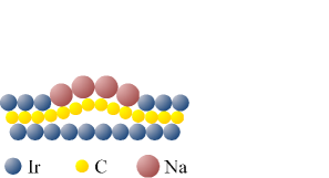
Figure 1: Schematic sketch of the Na/Ir/G sample.

The process was finely controlled to saturate the hcp regions of the Moiré-derived graphene supercells with one Ir cluster and to avoid cluster percolation. The optimal Ir coverage was determined to be 0.15 ML (monolayer) Ir, with reference to the density of an Ir(111) plane [acsnano, ; x1, ]. Additional Na was evaporated from a commercial getter source at room temperature and adsorbed to fill the residual exposed graphene surface. The resulting system (Na/Ir/G) was characterized by means of angle-resolved photoemission, as reported in Ref. [acsnano, ]. The valence band photoemission analysis was carried out by a Scienta R4000 electron energy analyzer with $120$ eV photons, close to the Cooper minimum of the Ir5d levels. The spectra were collected at 120 K with energy and angular resolution of 30 meV and 0.3^∘, respectively.

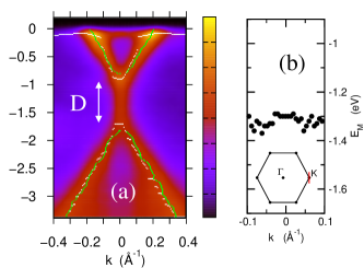
Figure 2: (a) ARPES intensity map of the electronic dispersion of Na/Ir/G along the direction p$\Gamma$K. The light green points represent the electronic dispersion determined by the momentum distribution curves, while white points the electronic dispersion obtained by energy distribution curves. The vertical white double arrow marks the magnitude $\Delta$ of the gap. The location of the cut p$\Gamma$K within the Brillouin zone is shown in the inset of panel (b). (b) Momentum dependence of the average $E_{\rm M,k}$ (see text).

The ARPES intensity map, along the direction perpendicular to $\Gamma$K passing through the K point (p$\Gamma$K) is shown in Fig. 2a, where the white and green symbols represent the position of the maxima in the energy-distribution-curves (EDCs) and in the momentum-distribution-curves (MDCs), respectively. The Fermi momentum along the p$\Gamma$K direction is $k_{\rm F}\approx 0.19$ Å^-1 that, taking into account the trigonal warping of the bands, gives an electron doping of $n\approx 0.028$ electrons per C atom. From the EDC at ${\bf k}=0$ we estimate a bandgap $\Delta\approx 0.8$ eV.

Two remarkable features stand out from the ARPES data: ($i$) both conduction and valence bands present a linear dispersion throughout the probed ${\bf k}$-space region, except within a very small region $k\lesssim 0.026$ Å^-1. This range is thus much smaller than that predicted by the massive gap model ($k\lesssim\Delta/\hbar v\approx 0.075$ Å^-1); ($ii$) the linear extrapolations of the upper and lower branched do not match, at variance with the expectations of the massive gap model. We note additionally the lack of any diamond-like features close to the K point, which would be typical trademarks of plasmaronic coupling [eli1, ; eli2, ; eli3, ; eli4, ; eli5, ; eli6, ]. On the other hand, plasmaron signatures in ARPES data have been so far reported only for epitaxial graphene on SiC, whereas they are absent in graphene grown on metallic substrates, most probably as a consequence of screening effects.

Such band structure of the Na/Ir/G system appears to be incompatible with the standard massive gap model, whereas they could be naturally reproduced within the context of the massless gap model.

In order to address at a more quantitative level this issue, we provide here a detailed careful analysis of the ARPES data for Na/Ir/G. Before testing the different models, it is necessary to estimate the basic parameters which are independent of the model itself, e.g. the Fermi velocity $v$ and the the Dirac energy $E_{\rm D}$ in the absence of the gap.

We estimate $\hbar v$ from the linear behavior of the lower band in the energy window from $-3.5$ eV to $-1.7$ eV, which yields $\hbar v\approx 5.3$ eV/Å. This value is consistent with the speed value derived from the upper band. We found this value was also perfectly compatible with the linear slope of the upper band. A rough estimate $E_{\rm D}=-1.3$ eV of the Dirac energy in the absence of the gap is obtained as the midgap point at ${\bf k}=0$ ($E_{k=0,+}=-0.9$ eV, $E_{k=0,-}=-1.7$ eV). This estimate can be cross-checked with the average energy between the upper and lower band $E_{\rm M,k}=(E_{k=0,-}+E_{k=0,-})/2$ for generic ${\bf k}$, displayed in Fig. 2b. The result shows a negligible momentum dependence, resulting in $E_{\rm M,k}=-1.3$ eV. Note that the negligible dependence of $E_{\rm M,k}$ on ${\bf k}$ signalizes an almost perfect symmetry of the experimental upper and lower bands with respect to the Dirac energy. This is compatible with both the massless and massive gap models, but it rules out plasmaronic effects which would result in an asymmetry and in a finite ${\bf k}$ dependence of $E_{\rm M,k}$.

The unbiased determination of $E_{\rm D}$ and $v$ allows to test the validity of the different models on the experimental data.

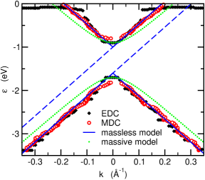
Figure 3: Comparison between the experimental dispersion for Na/Ir/G and the model predictions. Black filled diamonds and red empty circles represent EDC and MDC data, respectively. Solid blue lines the predictions of the massless model with $\Delta=0.3$ eV, and blue dashed lines the corresponding extrapolations of the Dirac cones. The dotted green lines show the massive gap model with $\Delta=0.4$ eV. In both theoretical cases we have used $E_{\rm D}=-1.3$ eV and $\hbar v\approx 5.3$ eV/Å.

Fig. 3 compares the band dispersion extracted from the momentum and energy distribution curves with the prediction of massless and massive modes. The best agreement is found for the massless model with $\Delta=0.3$ eV. Note the mismatch between the upper and lower Dirac cones, that reproduce perfectly the experimental data. The same value of the gap can be indeed also inferred from such misalignment. On the other hand, no satisfactory fit was possible for the massive model. We show here thus the predictions of the massive model for $\Delta=0.4$ eV, that reproduces the value at K of the upper and lower bands.

IV Microscopic models

In the previous section we have shown how a careful analysis of the band anomalies observed by ARPES in in Na/Ir/G points out towards a phenomenology of the graphene bands compatible more with massless gap model rather than with the standard massive one. It is clear that the different models represent a trademark for different underlying physical processes. In this Section we address thus this issue, in order to clarify which kind of physical processes can be responsible at the microscopic level for the massless Dirac phenomenology, with the final aim to control and engineering such processes.

Along this perspective, a brief summary of the microscopic physics related to the massive model can be useful. As mentioned in the Introduction, the massive Dirac model essentially stems from the presence of a local potential term $\propto\hat{\sigma}_{z}$ which makes the two carbon atom sublattices inequivalent. This potential can be naturally induced by the interaction of graphene with the substrate. The term $\Delta\hat{\sigma}_{z}$ in the Hamiltonian appears then as an external field arising from the environment. Alternatively, the onset of a mass term $\propto\hat{\sigma}_{z}$ has been discussed within the context of a spontaneous symmetry breaking, where the driving mechanism is the unscreened long-range Coulomb interaction [appel, ; khveshchenko1, ; khveshchenko2, ; vafek, ; juricic, ; drut, ; liu, ; gamayun, ; fertig1, ; gonzalez3, ; fertig2, ; kotov, ; gonzalez1, ; gonzalez2, ; wang, ; popovici, ]. The term $\Delta({\bf k})\hat{\sigma}_{z}$ can be viewed thus in this scenario as an anomalous self-energy term, i.e. as an order parameter, arising from many-body effects. It should be however mentioned that in this case the mass term $\Delta({\bf k})$ appears to be momentum dependent, i.e. divergent for ${\bf k}\rightarrow 0$ [gamayun, ; khveshchenko1, ], rather than ${\bf k}$-independent.

From a general point of view, since the presence of a linear Dirac cone in ideal flat graphene is dictated by symmetry reasons, it is clear that the opening of a gap and the splitting of the upper and lower bands, both in the massive and in the massless model, must be associated with some kind of breaking symmetry. We have indeed just seen how the symmetry breaking (spontaneous or not) responsible for the massive model is the equivalence between the local potentials of the two sublattices. In Ref. [bc, ] the general constraints that a phenomenological self-energy must satisfied to give rise to a massless Dirac model have been discussed. It is on the other hand intriguing to discuss in the present work the conditions that could make possible the appearance of a self-energy (14) as result of a tendency towards a spontaneous symmetry breaking.

It is clear that the effective breaking of symmetry, in real materials, can be prevented by many causes. For instance, as we will discuss below, a good candidate for a quasi-breaking of symmetry is the long-range Coulomb interaction. In real materials, and in particular in Na/Ir/graphene, such interaction is expected to be screened resulting in a cut-off of the singular behavior for small exchange momenta ${\bf q}$. Asymptotically, this should correspond to “regularization” of the interaction, and thus to a linear behavior of the dispersion (although with a very steep slope) for momenta ${\bf k}$ close to the K point. For larger ${\bf k}$, however, the tendency towards an instability can still be reflected in a quasi-gapped dispersion which can be compatible with the experimental observations. From this point of view, we present the analysis of the onset of a spontaneous symmetry breaking just as an illustrative example for the gross features of the resulting phenomenology. In similar way, we do not want to provide here a quantitative evaluation of the possible critical couplings required to induce a massless gapped case, rather to compare, at a qualitative level, this strength of this instability with the strength of the corresponding instability associated with the spontaneous generation of a mass according the model (1). In order to have thus a direct and clear way to compare the two possible instabilities, we address here this issue within the context of a mean-field solution, keeping in mind that a more compelling high-order analysis is needed for a quantitative investigation.

In order to address this issue in the most convenient way, we introduce the Nambu notation where the Hamiltonian of ideal free-standing graphene can be written as:

$$H = \sum_{{\bf k},\sigma}\psi_{{\bf k},\sigma}^{\dagger}\hat{H}_{0}({\bf k})\psi_{{\bf k},\sigma},$$ (16)

where $\sigma$ is a global index taking into account both spin and valley (degenerate) degrees of freedom $N_{s}=2$, $N_{v}=2$), $\psi_{{\bf k},\sigma}^{\dagger}$ is the spinor in the sublattice basis $\psi_{{\bf k},\sigma}^{\dagger}=(c_{{\bf k},\sigma,\rm A}^{\dagger},c_{{\bf k},\sigma,\rm B}^{\dagger})$, and where

$$\hat{H}_{0}({\bf k}) = \hbar vk\left[\hat{\sigma}_{x}\cos\theta+\hat{\sigma}_{y}\sin\theta\right].$$ (17)

We assume a long-range Coulomb interaction which can we written in the momentum space as:

$$H_{\rm C} = \frac{1}{2}\sum_{\sigma,\sigma^{\prime}}\sum_{\bf k,p,q}\rho_{\bf-q}V({\bf q})\rho_{\bf q},$$ (18)

where $\rho_{\bf q}=\sum_{{\bf k},\sigma}\psi_{{\bf k+q},\sigma}^{\dagger}\psi_{{\bf k},\sigma}$, and where $V({\bf q})=2\pi e^{2}[1-\delta({\bf q})]/\epsilon_{0}\kappa|{\bf q}|$. The term $\propto[1-\delta({\bf q})]$ in $V({\bf q})$ takes into account the subtraction of the positive charged background, while $\kappa$ is the dimensionless relative in-plane dielectric constant.

The phenomenology of the normal state self-energy arising from such many-body interaction, as well as of several possible anomalous self-energies associated with different spontaneous symmetry breaking, has been discussed in an extended way using different accurate techniques, as for instance renormalization group (RG) or static random-phase approximation (RPA). In general, in order to have an accurate estimate of the magnitude of the corresponding self-energies (and of the minimum strength of the interaction in the case of spontaneous symmetry breaking), a self-consistent screening of the quasi-particle excitations and of the the effective screened Coulomb interaction is required.

On the other hand, a qualitative insight on the matrix/momentum structure of the possible anomalous self-energies is already possible employing a simple mean-field treatment.

Neglecting the Hartree term, which does not play any role in the present context, and focusing on the exchange (Fock) term, we can write the generic self-energy as:

$$\hat{\Sigma}({\bf k}) = T\sum_{{\bf p},n}\frac{V({\bf k-p})}{i\omega_{n}\hat{I}-\hat{H}_{0}({\bf k})-\hat{\Sigma}({\bf k})}.$$ (19)

Note that, since the interaction $V({\bf q})$ is peaked at small ${\bf q=k-p}$, the intra-valley scattering is dominant, supporting the validity of the low-energy model versus a full tight-binding treatment. Note also that at this level of approximation (unscreened static Coulomb interaction) the self-energy does not depend on the frequency $i\omega_{n}$. Within this scheme is thus convenient to define an effective mean-field hamiltonian $\hat{H}({\bf k})=\hat{H}_{0}({\bf k})+\hat{\Sigma}({\bf k})$, and to write a recursive equation:

$$\hat{H}({\bf k}) = \hat{H}_{0}({\bf k})+T\sum_{{\bf p},n}\frac{V({\bf k-p})}{i\omega_{n}\hat{I}-\hat{H}({\bf k})}.$$ (20)

Since $V({\bf k-p})$ depends on the angular variables $\theta_{k}$, $\theta_{p}$ essentially through only $\cos(\theta_{k}-\theta_{p})$, one can see that $\hat{H}({\bf k})\approx\beta(k)[\hat{\sigma}_{x}\cos\theta+\hat{\sigma}_{y}\sin\theta$. Apart numerical prefactor, the momentum dependence of $\beta(k)$ on $k$ can be caught already by a perturbative analysis. Replacing $\hat{H}({\bf k})$ with $\hat{H}_{0}({\bf k})$ in the right side term of Eq. (20), or, equivalently, neglecting $\hat{\Sigma}({\bf k})$ in the right side term of Eq. (19), we obtain:

$$\beta(k) = \hbar vk\left[1+\frac{\alpha}{2\kappa}\gamma(k)\right]$$ (21)

where $\alpha=e^{2}/\epsilon_{0}\hbar v$ is the coupling constant for suspended graphene, ${\cal K}$ is a high-momentum cut-off limiting the validity of the Dirac model, approximately determined by the size of the Brillouin zone, and where

$$\gamma(k) = \int_{0}^{{\cal K}/k}dx\int_{0}^{2\pi}\frac{d\theta}{2\pi}\frac{x\cos\theta}{\sqrt{1+x^{2}-2x\cos\theta}}.$$ (22)

A careful analysis of (22) shows that at the leading order $\gamma(k)\approx(1/2)\ln({\cal K}/k)+$const., a well known result. Note that, within this context, the self-energy associated with the massless gap model is formally described by $\beta(k)=$const., i.e. by $\gamma(k)=1/k$. It is clear that such analytical dependence is not spontaneously generated by the self-consistent solution of (20) in the normal state, and it must be regarded as an order parameter of a possible second order phase transition. In order to address this possibility, we rewrite Eq. (20) as:

$$\hat{H}({\bf k})-\hat{W}[{\bf k},\{\hat{H}({\bf p})\}] = \hat{H}_{0}({\bf k}),$$ (23)

where $\hat{W}[{\bf k},\{\hat{X}\}]$ is the functional $\hat{W}[{\bf k},\{\hat{X}\}]=T\sum_{{\bf p},n}V({\bf k-p})/[i\omega_{n}\hat{I}-\hat{X}]$. Broken symmetry phases can be generated when the equation

$$\hat{\phi}({\bf k})-\hat{W}[{\bf k},\{\hat{H}({\bf p})+\hat{\phi}({\bf p})\}] = 0$$ (24)

admits a non-trivial solution $\hat{\phi}({\bf k})\neq 0$. We are here interested only in investigating the instability of the normal state towards a broken symmetry phase. Within this context we can expand thus the right side term of Eq. (24) at the linear order with respect to $\phi({\bf k})$. At $T=0$ we get thus the susceptibility equations:

$$\hat{\phi}({\bf k}) = \sum_{\bf p}V({\bf k-p})\frac{\hat{\phi}({\bf p})}{2E({\bf p})},$$ (25)

where $E({\bf p})={\rm det}[\hat{H}({\bf p})]$ is the energy dispersion in the normal state. Within the spirit of a mean-field approach we can neglect in $E({\bf p})$ the self-energy many-body effects driven by the Coulomb interactions, and approximate $E({\bf p})\simeq{\rm det}[\hat{H}_{0}({\bf p})]=\hbar v|{\bf p}|$. Eq. (25) can be used to investigate the instability towards both a massive as well as massless gap. In the first case $\hat{\phi}({\bf k})\propto\hat{\sigma}_{z}$, which clearly breaks the symmetry of the original Hamiltonian, while in the second case $\hat{\phi}({\bf k})\propto\hat{\sigma}_{x},\hat{\sigma}_{y}$. Since terms $\propto\hat{\sigma}_{x},\hat{\sigma}_{y}$ are already present in the normal state, it is not straightforwardly apparent at this level the nature of the symmetry breaking. On this regards it should be noticed that in the massless gap model the symmetry breaking is more specifically associated with the anomalous ${\bf k}$-dependence of the order parameter, in similarity with ${\bf q}=0$ flux phases discussed in different contexts, rather than with the Pauli structure.

To make clearer this point, we employ the massless gap model $\phi_{\rm ml}({\bf k})=\Delta_{\rm ml}[\hat{\sigma}_{x}\cos\theta+\hat{\sigma}_{y}\sin\theta]$ as an ansatz for the right side of Eq. (25). It is easy to check that the equations for $\hat{\sigma}_{x}$, $\hat{\sigma}_{y}$ result to be decoupled and degenerate. From a careful analysis of the angular variable, it is also straightforward to check that the resulting $\phi({\bf k})$ in the left side of Eq. (25) appears to be indeed $\phi({\bf k})=\beta_{\rm ml}(k)[\hat{\sigma}_{x}\cos\theta+\hat{\sigma}_{y}\sin\theta]$, where the prefactor $\beta_{\rm ml}(k)$ will be determined by the effective self-consistency of Eq. (25). Using the explicit expression for the Coulomb interaction, we obtain thus:

$$\beta_{\rm ml}(k) = \Delta_{\rm ml}\frac{\alpha}{2\kappa}$$ (26)

$$\times\int_{0}^{\cal K}dp\int_{0}^{2\pi}d\theta\frac{\cos\theta}{\sqrt{k^{2}+p^{2}-2kp\cos\theta}}.$$

It is remarkably relevant to notice that, contrary to Eq. (22), the integral over $p$ is well behaved for both $k\rightarrow 0$ and ${\cal K}\rightarrow\infty$. In this limits we can thus properly look for the self-consistent solution $\beta_{\rm ml}(k)=\Delta_{\rm ml}$. We obtain thus the susceptibility equation:

$$1 = \frac{\alpha}{2\kappa}\chi_{\rm ml}$$ (27)

where

$$\chi_{\rm ml} = \int_{0}^{\infty}dx\int_{0}^{2\pi}\frac{d\theta}{2\pi}\frac{\cos\theta}{\sqrt{1+x^{2}-2x\cos\theta}}$$ (28)

$$= \left[2-\sqrt{3}/2\right]\simeq 1.13.$$

For free-standing graphene with $\kappa=1$ we can predict thus a finite critical coupling $\alpha_{c}^{\rm ms}\simeq 1.76$ above which the system undergoes spontaneously a transition towards a massless gap phase.

We should stress that such value of $\alpha_{c}^{\rm ms}$ has been derived within the lowest order approximation, and a more compelling analysis is needed for a reliable quantitative estimate. It is however instructive to compare such value with the critical coupling required to induce, at the same level of approximation, a spontaneous generation of mass. Such instability can be determined by using the ansatz $\phi_{\rm ms}({\bf k})=[\Delta_{\rm ms}/\sqrt{k}]\hat{\sigma}_{z}$ in Eq. (25). After few straightforward steps, we obtain the susceptibility equation

$$1 = \frac{\alpha}{2\kappa}\chi_{\rm ms}$$ (29)

where

$$\chi_{\rm ms} = \int_{0}^{\infty}\frac{dx}{\sqrt{x}}\int_{0}^{2\pi}\frac{d\theta}{2\pi}{\sqrt{1+x^{2}-2x\cos\theta}}$$ (30)

$$= \frac{\Gamma^{4}(1/4)}{4\pi^{2}}\simeq 4.38,$$

corresponding, for $\kappa=1$, to the well-known result $\alpha_{c}^{\rm ms}\simeq 0.46$ [gamayun, ; popovici, ].

Although the critical coupling $\alpha_{c}^{\rm ml}$ for the spontaneous generation of massless gap results to be larger than the critical coupling for the massive gap, it remains still of the same order of magnitude of $\alpha_{c}^{\rm ms}$ within the same level of approximation. We know however that $\alpha_{c}^{\rm ms}$ is significantly increased when higher order renormalization effects (dynamical screening, self-energy effects, …) are taken into account, with possible $\alpha_{c}^{\rm ms}$ as large as $\alpha_{c}^{\rm ms}\approx 2$, of the same order thus of the present estimate of $\alpha_{c}^{\rm ml}$. Becomes thus crucial, in order to assess the dominant instability of the normal state, to include high-order effect also for the massless gap case, to permit a quantitative comparison. In addition, it should not be excluded a possible interplay, in the broken symmetry phase, between the two order parameters, where one could favor and make more stable the other one. This scenario is suggested by the simple analysis of the experimental data of Fig. 3, where the massless gap model reproduce well the experimental dispersion in a broad energy range, but where a finite parabolic behavior is nevertheless present at very small $k$. We have already discuss how such weak parabolic behavior cannot account in any case for the large observed gap. The experimental dispersion could be thus compatible with the possible coexistence of the both qualitatively different gaps, with the massless (larger) one determining the high-energy range, and the massive (smaller) one accounting for the residual parabolic behavior at small $k$. Further analysis in this direction is however needed to investigate this issue.

In conclusion, in this work we have provided, using angle-resolved photoemission spectroscopy, a compelling evidence of the presence of an unconventional gap in CVD grown graphene, properly described by a massless gap model. We have further investigated, on a theoretical ground, the microscopic conditions that can give rise to a spontaneous phase transition towards such massless gapped phase. We have shown that, for suspended graphene, a critical value of the Coulomb coupling is needed, with larger but comparable values with the ones required to induce a breaking symmetry towards a massive map. This analysis, stricty valid for suspended graphene, can suggest a possible path to induce such unconventional gap also in CVD graphene, although in this case specific features of these materials (screening of the Coulomb interaction, interference with the Moiré pattern) must be taken into account. The fully understanding and controlling of the unconventional properties of the massless gap in graphene can open new perspectives in the bandgap engineering in graphene-based materials.

Acknowledgements

E.C. acknowledges support from the European project FP7-PEOPLE-2013-CIG ”LSIE_2D” and Italian National MIUR Prin project 20105ZZTSE. L.B. acknowledges support from the Italian MIUR under the projects FIRB-HybridNanoDev-RBFR1236VV and PRIN-2012X3YFZ2. Financial support was also provided by Italian MIUR project FIRB-Futuro in Ricerca 2010-Project Plasmograph Grant No. RBFR10M5BT.

References

- (1) For a review about physical properties of graphene see for instance: A.H. Castro Neto, F. Guinea, N.M.R. Peres, K.S. Novoselov, and A.K. Geim, Rev. Mod. Phys. 81, 109 (2009), and references tehrein.
- (2) K.R. Knox et al., Phys. Rev. B 84, 115401 (2011).
- (3) S. Y. Zhou, G. -H. Gweon, A. V. Fedorov, P. N. First, W. A. de Heer, D. -H. Lee, F. Guinea, A. H. Castro Neto, and A. Lanzara, Nat. Mat. 6, 770 (2007).
- (4) S.Y. Zhou, D.A. Siegel, A.V. Fedorov, and A. Lanzara, Physica E 4, 2642 (2008).
- (5) X. Liang et al., Nano Lett. 10, 2454 (2010).
- (6) J. Bai et al., Nat. Nanotechnol. 5, 190 (2010).
- (7) T.G. Pedersen et al., Phys. Rev. Lett. 100, 136804 (2008).
- (8) F. Yavari et al., Small 6, 2535 (2010).
- (9) C.H. Park et al., Nano Lett. 8, 2200 (2008).
- (10) R. Balog et al., Nat. Mater. 9, 315 (2010).
- (11) D. Haberer et al., Nano Lett. 10, 3360 (2010).
- (12) A. Varykhalov et al., Phys. Rev. B 82, 121101 (2010).
- (13) Z.H. Ni et al., ACS Nano 11, 2301 (2008).
- (14) S. Rusponi et al., Phys. Rev. Lett. 105, 246803 (2010).
- (15) C. Jeon et al., Sci. Rep. 3, 2725 (2013).
- (16) M. Scardamaglia et al., J. Phys. Chem. C 117, 3019 (2013);
- (17) M. Papagno, S. Rusponi, P.M. Sheverdyaeva, S. Vlaic, M. Etzkorn, D. Pacilé , P. Moras, C. Carbone, and H. Brune, ACS Nano 6, 199 (2012).
- (18) A. Bostwick, T. Ohta, T. Seyller, K. Horn, and E. Rotenberg, Nat. Phys. 3, 36 (2007).
- (19) A. Bostwick, T. Ohta, J. L. McChesney, K. V. Emtsev, T. Seyller, K. Horn, and E. Rotenberg, New J. Phys. 9, 385 (2007).
- (20) E. Rotenberg, A. Bostwick, T. Ohta, J. L. McChesney, Th. Seyller, and K. Horn, Nat. Mater. 7, 258 (2008).
- (21) A.L. Walter et al., Phys. Rev. B 84, 085410 (2011).
- (22) A. Bostwick et al., Science 328, 999 (2010).
- (23) A. Principi, R. Asgari, and M. Polini, Solid State Commun. 151, 1627 (2011).
- (24) L. Benfatto and E. Cappelluti, Phys. Rev. B 78, 115434 (2008).
- (25) M. Mucha-Kruczynski, O. Tsyplyatyev, A. Grishin, E. McCann, V.I. Fal’ko, A. Bostwick, and E. Rotenberg, Phys. Rev. B 77, 195403 (2008).
- (26) T. Appelquist, D. Nash, and L.C.R. Wijewardhana, Phys. Rev. Lett. 60, 2575 (1988).
- (27) D.V. Khveshchenko, Phys. Rev. Lett. 87, 246802 (2001).
- (28) D. V. Khveshchenko and H. Leal, Nucl. Phys. B 687, 323 (2004).
- (29) O. Vafek and M.J. Case, Phys. Rev. B 77, 033410 (2008).
- (30) V. Juricic, I.F. Herbut, and G.W. Semenoff, Phys. Rev. B 80, 081405 (2009).
- (31) J.E. Drut and T.A. Lädhe, Phys. Rev. B 79, 165425 (2009).
- (32) Guo-Zhu Liu, Wei Li, and Geng Cheng Phys. Rev. B 79, 205429 (2009).
- (33) O.V. Gamayun, E.V. Gorbar, and V.P. Gusynin, Phys. Rev. B 80, 165429 (2009).
- (34) J. Wang, H.A. Fertig, and G. Murthy, Phys. Rev. Lett. 104, 186401 (2010).
- (35) J. González, Phys. Rev. B 82, 155404 (2010).
- (36) J. Wang, H.A. Fertig, G. Murthy, and L. Brey, Phys. Rev. B 83, 035404 (2011).
- (37) V.N. Kotov, B. Uchoa, V.M. Pereira, A.H. Castro Neto, and F. Guinea, Rev. Mod. Phys. 84, 1067 (2012).
- (38) J. González, Phys. Rev. B 85, 085420 (2012).
- (39) J. González, JHEP 08, 27 (2012); arXiv.:1204.4673 (2012).
- (40) J.-R. Wang and G.-Z. Liu, New J. Phys. 14, 043036 (2012).
- (41) C. Popovici, C.S. Fischer, and L. von Smekal, Phys. Rev. B 88, 205429 (2013);
- (42) J. González, F. Guinea, and M.A.H. Vozmediano, Phys. Rev. B 59, R2474 (1999).
- (43) E.G. Mishchenko, Phys. Rev. Lett. 98, 216801 (2007).
- (44) A.T. N’Diaye, S. Bleikamp, P.J. Feibelman, and T. Michely, Phys. Rev. Lett. 97, 215501 (2006).