Euclidean Distance Matrices
Essential Theory, Algorithms and Applications

Abstract

Euclidean distance matrices (EDM) are matrices of squared distances between points. The definition is deceivingly simple: thanks to their many useful properties they have found applications in psychometrics, crystallography, machine learning, wireless sensor networks, acoustics, and more. Despite the usefulness of EDMs, they seem to be insufficiently known in the signal processing community. Our goal is to rectify this mishap in a concise tutorial.

We review the fundamental properties of EDMs, such as rank or (non)definiteness. We show how various EDM properties can be used to design algorithms for completing and denoising distance data. Along the way, we demonstrate applications to microphone position calibration, ultrasound tomography, room reconstruction from echoes and phase retrieval. By spelling out the essential algorithms, we hope to fast-track the readers in applying EDMs to their own problems. Matlab code for all the described algorithms, and to generate the figures in the paper, is available online. Finally, we suggest directions for further research.

I Introduction

Imagine that you land at Geneva airport with the Swiss train schedule but no map. Perhaps surprisingly, this may be sufficient to reconstruct a rough (or not so rough) map of the Alpine country, even if the train times poorly translate to distances or some of the times are unknown. The way to do it is by using Euclidean distance matrices (EDM): for a quick illustration, take a look at the “Swiss Trains” box.

An EDM is a matrix of squared Euclidean distances between points in a set. We often work with distances because they are convenient to measure or estimate. In wireless sensor networks for example, the sensor nodes measure received signal strengths of the packets sent by other nodes, or time-of-arrival (TOA) of pulses emitted by their neighbors [1]. Both of these proxies allow for distance estimation between pairs of nodes, thus we can attempt to reconstruct the network topology. This is often termed self-localization [2, 3, 4]. The molecular conformation problem is another instance of a distance problem [5], and so is reconstructing a room’s geometry from echoes [6]. Less obviously, sparse phase retrieval [7] can be converted to a distance problem, and addressed using EDMs.

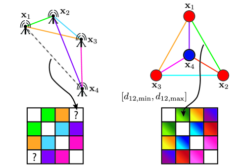
Figure 1: Two real-world applications of EDMs. Sensor network localization from estimated pairwise distances is illustrated on the left, with one distance missing because the corresponding sensor nodes are too far apart to communicate. In the molecular conformation problem on the right, we aim to estimate the locations of the atoms in a molecule from their pairwise distances. Here, due to the inherent measurement uncertainty, we know the distances only up to an interval.

Sometimes the data are not metric, but we seek a metric representation, as it happens commonly in psychometrics [8]. As a matter of fact, the psychometrics community is at the root of the development of a number of tools related to EDMs, including multidimensional scaling (MDS)—the problem of finding the best point set representation of a given set of distances. More abstractly, people are concerned with EDMs for objects living in high-dimensional vector spaces, such as images [9].

EDMs are a useful description of the point sets, and a starting point for algorithm design. A typical task is to retrieve the original point configuration: it may initially come as a surprise that this requires no more than an eigenvalue decomposition (EVD) of a symmetric matrix. In fact, the majority of Euclidean distance problems require the reconstruction of the point set, but always with one or more of the following twists:

1. Distances are noisy,

2. Some distances are missing,

3. Distances are unlabeled.

For two examples of applications requiring a solution of EDM problems with different complications, see Fig. 1.

Swiss Trains (Swiss Map Reconstruction)

Consider the following matrix of times in minutes it takes to travel by train between some Swiss cities:

$$\bordermatrix{&\text{L}&\text{G}&\text{Z}&\text{N}&\text{B}\cr\text{Lausanne}&0&33&128&40&66\cr\text{Geneva}&33&0&158&64&101\cr\text{Z\"{u}rich}&128&158&0&88&56\cr\text{Neuch\^{a}tel}&40&64&88&0&34\cr\text{Bern}&66&101&56&34&0\cr}$$

The numbers were taken from the Swiss railways timetable. The matrix was then processed using the classical MDS algorithm (Algorithm 1), which is basically an EVD. The obtained city configuration was rotated and scaled to align with the actual map. Given all the uncertainties involved, the fit is remarkably good. Not all trains drive with the same speed; they have varying numbers of stops, railroads are not straight lines (lakes and mountains). This result may be regarded as anecdotal, but in a fun way it illustrates the power of the EDM toolbox. Classical MDS could be considered the simplest of the available tools, yet it yields usable results with erroneous data. On the other hand, it might be that Swiss trains are just so good.

There are two fundamental problems associated with distance geometry [10]: (i) given a matrix, determine whether it is an EDM, (ii) given a possibly incomplete set of distances, determine whether there exists a configuration of points in a given embedding dimension—dimension of the smallest affine space comprising the points—that generates the distances.

I-A Prior Art

The study of point sets through pairwise distances, and so of EDMs, can be traced back to the works of Menger [11], Schoenberg [12], Blumenthal [13], and Young and Householder [14].

An important class of EDM tools was initially developed for the purpose of data visualization. In 1952, Torgerson introduced the notion of MDS [8]. He used distances to quantify the dissimilarities between pairs of objects that are not necessarilly vectors in a metric space. Later in 1964, Kruskal suggested the notion of stress as a measure of goodness-of-fit for non-metric data [15], again representing experimental dissimilarities between objects.

A number of analytical results on EDMs were developed by Gower [16, 17]. In his 1985 paper [17], he gave a complete characterization of the EDM rank. Optimization with EDMs requires good geometric intuitions about matrix spaces. In 1990, Glunt [18] and Hayden [19] with their co-authors provided insights into the structure of the convex cone of EDMs. An extensive treatise on EDMs with many original results and an elegant characterization of the EDM cone is given by Dattorro [20].

In early 1980s, Williamson, Havel and Wüthrich developed the idea of extracting the distances between pairs of hydrogen atoms in a protein, using nuclear magnetic resonance (NMR). The extracted distances were then used to reconstruct 3D shapes of molecules [5]. The NMR spectrometer (together with some post-processing) outputs the distances between pairs of atoms in a large molecule. The distances are not specified for all atom pairs, and they are uncertain—given only up to an interval. This setup lends itself naturally to EDM treatment; for example, it can be directly addressed using MDS [21]. Indeed, the crystallography community also contributed a large number of important results on distance geometry. In a different biochemical application, comparing distance matrices yields efficient algorithms for comparing proteins from their 3D structure [22].

In machine learning, one can learn manifolds by finding an EDM with a low embedding dimension that preserves the geometry of local neighborhoods. Weinberger and Saul use it to learn image manifolds [9]. Other examples of using Euclidean distance geometry in machine learning are results by Tenenbaum, De Silva and Langford [23] on image understanding and handwriting recognition, Jain and Saul [24] on speech and music, and Demaine and et al. [25] on music and musical rhythms.

With the increased interest in sensor networks, several EDM-based approaches were proposed for sensor localization [2, 3, 4, 20]. Connections between EDMs, multilateration and semidefinite programming are expounded in depth in [26], especially in the context of sensor network localization.

Position calibration in ad-hoc microphone arrays is often done with sources at unknown locations, such as handclaps, fingersnaps or randomly placed loudspeakers [27, 28, 29]. This gives us distances (possibly up to an offset time) between the microphones and the sources and leads to the problem of multi-dimensional unfolding [30].

All of the above applications work with labeled distance data. In certain TOA- based applications one loses the labels—the correct permutation of the distances is no longer known. This arises in reconstructing the geometry of a room from echoes [6]. Another example of unlabeled distances is in sparse phase retrieval, where the distances between the unknown non-zero lags in a signal are revealed in its autocorrelation function [7]. Recently, motivated by problems in crystallography, Gujarahati and co-authors published an algorithm for reconstruction of Euclidean networks from unlabeled distance data [31].

I-B Our Mission

We were motivated to write this tutorial after realizing that EDMs are not common knowledge in the signal processing community, perhaps for the lack of a compact introductory text. This is effectively illustrated by the anecdote that, not long before writing this article, one of the authors had to add the (rather fundamental) rank property to the Wikipedia page on EDMs. In a compact tutorial we do not attempt to be exhaustive; much more thorough literature reviews are available in longer exposés on EDMs and distance geometry [10, 32, 33]. Unlike these works that take the most general approach through graph realizations, we opt to show simple cases through examples, and to explain and spell out a set of basic algorithms that anyone can use immediately. Two big topics that we discuss are not commonly treated in the EDM literature: localization from unlabeled distances, and multidimensional unfolding (applied to microphone localization). On the other hand, we choose to not explicitly discuss the sensor network localization (SNL) problem, as the relevant literature is abundant.

Implementations of all the algorithms are available online. Our hope is that this will provide a good entry point for those wishing to learn much more, and inspire new approaches to old problems.

TABLE I: Summary of notation

Symbol	Meaning
$n$	Number of points (columns) in $\bm{X}=[\bm{x}_{1},\ldots,\bm{x}_{n}]$
$d$	Dimensionality of the Euclidean space
$a_{ij}$	Element of a matrix $\bm{A}$ on the $i$th row and the $j$th column
$\bm{D}$	A Euclidean distance matrix
$\mathrm{edm}(\bm{X})$	Euclidean distance matrix created from columns in $\bm{X}$
$\mathrm{edm}(\bm{X},\bm{Y})$	Matrix containing the squared distances between the columns of $\bm{X}$ and $\bm{Y}$
$\mathcal{K}(\bm{G})$	Euclidean distance matrix created from the Gram matrix $\bm{G}$
$\bm{J}$	Geometric centering matrix
$\bm{A}_{\bm{W}}$	Restriction of $\bm{A}$ to non-zero entries in $\bm{W}$
$\bm{W}$	Mask matrix, with ones for observed entries
$\mathbb{S}_{+}^{n}$	Set of real symmetric positive semidefinite matrices in $\mathbb{R}^{n\times n}$
$\mathrm{affdim}(\bm{X})$	Affine dimension of the points listed in $\bm{X}$
$\bm{A}\circ\bm{B}$	Hadamard (entrywise) product of $\bm{A}$ and $\bm{B}$
$\epsilon_{ij}$	Noise corrupting the $(i,j)$ distance
$\bm{e}_{i}$	$i$th vector of the canonical basis
$\left\lVert\bm{A}\right\rVert_{F}$	Frobenius norm of $\bm{A}$, $\big{(}\sum_{ij}a_{ij}^{2}\big{)}^{1/2}$

II From Points to EDMs and Back

The principal EDM-related task is to reconstruct the original point set. This task is an inverse problem to the simpler forward problem of finding the EDM given the points. Thus it is desirable to have an analytic expression for the EDM in terms of the point matrix. Beyond convenience, we can expect such an expression to provide interesting structural insights. We will define notation as it becomes necessary—a summary is given in Table I.

Consider a collection of $n$ points in a $d$-dimensional Euclidean space, ascribed to the columns of matrix $\bm{X}\in\mathbb{R}^{d\times n}$, $\bm{X}=[\bm{x}_{1},\ \bm{x}_{2},\ \cdots,\ \bm{x}_{n}],\ \bm{x}_{i}\in\mathbb{R}^{d}$. Then the squared distance between $\bm{x}_{i}$ and $\bm{x}_{j}$ is given as

$$d_{ij}=\left\lVert\bm{x}_{i}-\bm{x}_{j}\right\rVert^{2},$$ (1)

where $\left\lVert\,\cdot\,\right\rVert$ denotes the Euclidean norm. Expanding the norm yields

$$d_{ij}=(\bm{x}_{i}-\bm{x}_{j})^{\top}(\bm{x}_{i}-\bm{x}_{j})=\bm{x}_{i}^{\top}\bm{x}_{i}-2\bm{x}_{i}^{\top}\bm{x}_{j}+\bm{x}_{j}^{\top}\bm{x}_{j}.$$ (2)

From here, we can read out the matrix equation for $\bm{D}=[d_{ij}]$,

$$\mathrm{edm}(\bm{X})\overset{\text{def}}{=}\bm{\mathit{1}}\mathop{\mathrm{diag}}(\bm{X}^{\top}\bm{X})^{\top}-2\bm{X}^{\top}\bm{X}+\mathop{\mathrm{diag}}(\bm{X}^{\top}\bm{X})\bm{\mathit{1}}^{\top},$$ (3)

where $\bm{\mathit{1}}$ denotes the column vector of all ones and $\mathop{\mathrm{diag}}(\bm{A})$ is a column vector of the diagonal entries of $\bm{A}$. We see that $\mathrm{edm}(\bm{X})$ is in fact a function of $\bm{X}^{\top}\bm{X}$. For later reference, it is convenient to define an operator $\mathcal{K}(\bm{G})$ similar to $\mathrm{edm}(\bm{X})$, that operates directly on the Gram matrix $\bm{G}=\bm{X}^{\top}\bm{X}$,

$$\mathcal{K}(\bm{G})\overset{\text{def}}{=}\mathop{\mathrm{diag}}(\bm{G})\bm{\mathit{1}}^{\top}-2\bm{G}+\bm{\mathit{1}}\mathop{\mathrm{diag}}(\bm{G})^{\top}.$$ (4)

The EDM assembly formula (3) or (4) reveals an important property: Because the rank of $\bm{X}$ is at most $d$ (it has $d$ rows), then the rank of $\bm{X}^{\top}\bm{X}$ is also at most $d$. The remaining two summands in (3) have rank one. By rank inequalities, rank of a sum of matrices cannot exceed the sum of the ranks of the summands. With this observation, we proved one of the most notable facts about EDMs:

Theorem 1 (Rank of EDMs).

Rank of an EDM corresponding to points in $\mathbb{R}^{d}$ is at most $d+2$.

This is a powerful theorem: it states that the rank of an EDM is independent of the number of points that generate it. In many applications, $d$ is three or less, while $n$ can be in the thousands. According to Theorem 1, rank of such practical matrices is at most five. The proof of this theorem is simple, but to appreciate that the property is not obvious, you may try to compute the rank of the matrix of non-squared distances.

What really matters in Theorem 1 is the affine dimension of the point set—the dimension of the smallest affine subspace that contains the points, denoted by $\mathrm{affdim}(\bm{X})$. For example, if the points lie on a plane (but not on a line or a circle) in $\mathbb{R}^{3}$, rank of the corresponding EDM is four, not five. This will be clear from a different perspective in the next subsection, as any affine subspace is just a translation of a linear subspace. An illustration for a 1D subspace of $\mathbb{R}^{2}$ is provided in Fig. 2: Subtracting any point in the affine subspace from all its points translates it to the parallel linear subspace that contains the zero vector.

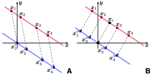
Figure 2: Illustration of the relationship between an affine subspace and its parallel linear subspace. The points $\bm{X}=[\bm{x}_{1},\ldots,\bm{x}_{4}]$ live in an affine subspace—a line in $\mathbb{R}^{2}$ that does not contain the origin. In (A), the vector $\bm{x}_{1}$ is subtracted from all the points, and the new point list is $\bm{X}^{\prime}=[\bm{\mathit{0}},\bm{x}_{2}-\bm{x}_{1},\bm{x}_{3}-\bm{x}_{1},\bm{x}_{4}-\bm{x}_{1}]$. While the columns of $\bm{X}$ span $\mathbb{R}^{2}$, the columns of $\bm{X}^{\prime}$ only span the 1D subspace of $\mathbb{R}^{2}$—the line through the origin. In (B), we subtract a different vector from all points: the centroid $\frac{1}{4}\bm{X}\bm{\mathit{1}}$. The translated vectors $\bm{X}^{\prime\prime}=[\bm{x}_{1}^{\prime\prime},\ldots,\bm{x}_{4}^{\prime\prime}]$ again span the same 1D subspace.

II-A Essential Uniqueness

When solving an inverse problem, we need to understand what is recoverable and what is forever lost in the forward problem. Representing sets of points by distances usually increases the size of the representation. For most interesting $n$ and $d$, the number of pairwise distances is larger than the size of the coordinate description, $\binom{n}{2}>nd$, so an EDM holds more scalars than the list of point coordinates. Nevertheless, some information is lost in this encoding, namely the information about the absolute position and orientation of the point set. Intuitively, it is clear that rigid transformations (including reflections) do not change distances between the fixed points in a point set. This intuitive fact is easily deduced from the EDM assembly formula (3). We have seen in (3) and (4) that $\mathrm{edm}(\bm{X})$ is in fact a function of the Gram matrix $\bm{X}^{\top}\bm{X}$.

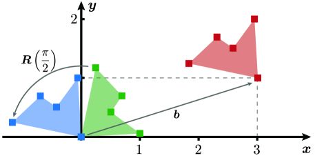
Figure 3: Illustration of a rigid transformation in 2D. Here the points set is transformed as $\bm{R}\bm{X}+\bm{b}\bm{\mathit{1}}^{\!\top}$. Rotation matrix $\bm{R}=\left[\begin{subarray}{c}\ \ 0\ 1\\ -1\ 0\end{subarray}\right]$, corresponds to a counterclockwise rotation of 90^∘. The translation vector is $\bm{b}=[3,\ 1]^{\top}$. The shape is drawn for visual reference.

This makes it easy to show algebraically that rotations and reflections do not alter the distances. Any rotation/reflection can be represented by an orthogonal matrix $\bm{Q}\in\mathbb{R}^{d\times d}$ acting on the points $\bm{x}_{i}$. Thus for the rotated point set $\bm{X}_{r}=\bm{Q}\bm{X}$ we can write

$$\bm{X}_{r}^{\top}\bm{X}_{r}=(\bm{Q}\bm{X})^{\top}(\bm{Q}\bm{X})=\bm{X}^{\top}\bm{Q}^{\top}\bm{Q}\bm{X}=\bm{X}^{\top}\bm{X},$$ (5)

where we invoked the orthogonality of the rotation/reflection matrix, $\bm{Q}^{\top}\bm{Q}=\bm{I}$.

Translation by a vector $\bm{b}\in\mathbb{R}^{d}$ can be expressed as

$$\bm{X}_{t}=\bm{X}+\bm{b}\bm{\mathit{1}}^{\top}.$$ (6)

Using $\mathop{\mathrm{diag}}(\bm{X}_{t}^{\top}\bm{X}_{t})=\mathop{\mathrm{diag}}(\bm{X}^{\top}\bm{X})+2\bm{X}^{\top}\bm{b}+\left\lVert b\right\rVert^{2}\bm{\mathit{1}}$, one can directly verify that this transformation leaves (3) intact. In summary,

$$\mathrm{edm}(\bm{Q}\bm{X})=\mathrm{edm}(\bm{X}+\bm{b}\bm{\mathit{1}}^{\top})=\mathrm{edm}(\bm{X}).$$ (7)

The consequence of this invariance is that we will never be able to reconstruct the absolute orientation of the point set using only the distances, and the corresponding degrees of freedom will be chosen freely. Different reconstruction procedures will lead to different realizations of the point set, all of them being rigid transformations of each other. Fig. 3 illustrates a point set under a rigid transformation. It is clear that the distances between the points are the same for all three shapes.

II-B Reconstructing the Point Set From Distances

The EDM equation (3) hints at a procedure to compute the point set starting from the distance matrix. Consider the following choice: let the first point $\bm{x}_{1}$ be at the origin. Then the first column of $\bm{D}$ contains the squared norms of the point vectors,

$$d_{i1}=\left\lVert\bm{x}_{i}-\bm{x}_{1}\right\rVert^{2}=\left\lVert\bm{x}_{i}-\bm{\mathit{0}}\right\rVert^{2}=\left\lVert\bm{x}_{i}\right\rVert^{2}.$$ (8)

Consequently, we can immediately construct the term $\bm{\mathit{1}}\mathop{\mathrm{diag}}(\bm{X}^{\top}\bm{X})$ and its transpose in (3), as the diagonal of $\bm{X}^{\top}\bm{X}$ contains exactly the norms squared $\left\lVert\bm{x}_{i}\right\rVert^{2}$. Concretely,

$$\bm{\mathit{1}}\mathop{\mathrm{diag}}(\bm{X}^{\top}\bm{X})=\bm{\mathit{1}}\bm{d}_{1}^{\top},$$ (9)

where $\bm{d}_{1}=\bm{D}\bm{e}_{1}$ is the first column of $\bm{D}$. We thus obtain the Gram matrix from (3) as

$$\bm{G}=\bm{X}^{\top}\bm{X}=-\frac{1}{2}(\bm{D}-\bm{\mathit{1}}\bm{d}_{1}^{\top}-\bm{d}_{1}\bm{\mathit{1}}^{\top}).$$ (10)

The point set can be found by an EVD, $\bm{G}=\bm{U}\bm{\mathit{\Lambda}}\bm{U}^{\top}$, where $\bm{\mathit{\Lambda}}=\mathop{\mathrm{diag}}(\lambda_{1},\ldots,\lambda_{n})$ with all eigenvalues $\lambda_{i}$ non-negative, and $\bm{U}$ orthonormal, as $\bm{G}$ is a symmetric positive semidefinite matrix. Throughout the paper we assume that the eigenvalues are sorted in the order of decreasing magnitude, $\left|\lambda_{1}\right|\geq\left|\lambda_{2}\right|\geq\cdots\geq\left|\lambda_{n}\right|$. We can now set $\widehat{\bm{X}}\overset{\text{def}}{=}\big{[}\mathop{\mathrm{diag}}\big{(}\sqrt{\lambda_{1}},\ \ldots,\ \sqrt{\lambda_{d}}\,\big{)},\ \bm{\mathit{0}}_{d\times(n-d)}\big{]}\bm{U}^{\top}$. Note that we could have simply taken $\bm{\mathit{\Lambda}}^{1/2}\bm{U}^{\top}$ as the reconstructed point set, but if the Gram matrix really describes a $d$-dimensional point set, the trailing eigenvalues will be zeroes, so we choose to truncate the corresponding rows.

It is straightforward to verify that the reconstructed point set $\widehat{\bm{X}}$ generates the original EDM, $\bm{D}=\mathrm{edm}(\bm{X})$; as we have learned, $\widehat{\bm{X}}$ and $\bm{X}$ are related by a rigid transformation. The described procedure is called the classical MDS, with a particular choice of the coordinate system: $\bm{x}_{1}$ is fixed at the origin.

In (10) we subtract a structured rank-2 matrix $(\bm{\mathit{1}}\bm{d}_{1}^{\top}+\bm{d}_{1}\bm{\mathit{1}}^{\top})$ from $\bm{D}$. A more systematic approach to the classical MDS is to use a generalization of (10) by Gower [16]. Any such subtraction that makes the right hand side of (10) positive semidefinite (PSD), i.e., that makes $\bm{G}$ a Gram matrix, can also be modeled by multiplying $\bm{D}$ from both sides by a particular matrix. This is substantiated in the following result.

Theorem 2 (Gower [16]).

$\bm{D}$ is an EDM if and only if

$$-\frac{1}{2}(\bm{I}-\bm{\mathit{1}}\bm{s}^{\top})\bm{D}(\bm{I}-\bm{s}\bm{\mathit{1}}^{\top})$$ (11)

is PSD for any $\bm{s}$ such that $\bm{s}^{\top}\bm{\mathit{1}}=1$ and $\bm{s}^{\top}\bm{D}\neq\bm{\mathit{0}}$.

In fact, if (11) is PSD for one such $\bm{s}$, then it is PSD for all of them. In particular, define the geometric centering matrix as

$$\bm{J}\overset{\text{def}}{=}\bm{I}-\frac{1}{n}\bm{\mathit{1}}\bm{\mathit{1}}^{\top}.$$ (12)

Then $-\frac{1}{2}\bm{J}\bm{D}\bm{J}$ being positive semidefinite is equivalent to $\bm{D}$ being an EDM. Different choices of $\bm{s}$ correspond to different translations of the point set.

The classical MDS algorithm with the geometric centering matrix is spelled out in Algorithm 1. Whereas so far we have assumed that the distance measurements are noiseless, Algorithm 1 can handle noisy distances too, as it discards all but the $d$ largest eigenvalues.

Algorithm 1 Classical MDS

• function ClassicalMDS($\bm{D},d$)

• $\bm{J}\leftarrow\bm{I}-\frac{1}{n}\bm{\mathit{1}}\bm{\mathit{1}}^{\top}$ $\triangleright$ Geometric centering matrix

• $\bm{G}\leftarrow-\frac{1}{2}\bm{J}\bm{D}\bm{J}$ $\triangleright$ Compute the Gram matrix

• $\bm{U},[\,\lambda_{i}\,]_{i=1}^{n}\leftarrow\mathrm{EVD}(\bm{G})$

• return $\big{[}\mathop{\mathrm{diag}}\big{(}\sqrt{\lambda_{1}},\ \ldots,\ \sqrt{\lambda_{d}}\,\big{)},\ \bm{\mathit{0}}_{d\times(n-d)}\big{]}\bm{U}^{\top}$

• end function

It is straightforward to verify that (10) corresponds to $\bm{s}=\bm{e}_{1}$. Think about what this means in terms of the point set: $\bm{X}\bm{e}_{1}$ selects the first point in the list, $\bm{x}_{1}$. Then $\bm{X}_{0}=\bm{X}(\bm{I}-\bm{e}_{1}\bm{\mathit{1}}^{\top})$ translates the points so that $\bm{x}_{1}$ is translated to the origin. Multiplying the definition (3) from the right by $(\bm{I}-\bm{e}_{1}\bm{\mathit{1}}^{\top})$ and from the left by $(\bm{I}-\bm{\mathit{1}}\bm{e}_{1}^{\top})$ will annihilate the two rank-1 matrices, $\mathop{\mathrm{diag}}(\bm{G})\bm{\mathit{1}}^{\top}$ and $\bm{\mathit{1}}\mathop{\mathrm{diag}}(\bm{G})^{\top}$. We see that the remaining term has the form $-2\bm{X}_{0}^{\top}\bm{X}_{0}$, and the reconstructed point set will have the first point at the origin!

On the other hand, setting $\bm{s}=\frac{1}{n}\bm{\mathit{1}}$ places the centroid of the point set at the origin of the coordinate system. For this reason, the matrix $\bm{J}=\bm{I}-\frac{1}{n}\bm{\mathit{1}}\bm{\mathit{1}}^{\top}$ is called the centering matrix. To better understand why, consider how we normally center a set of points given in $\bm{X}$.

First, we compute the centroid as the mean of all the points

$$\bm{x}_{c}=\frac{1}{n}\sum_{i=1}^{n}\bm{x}_{i}=\frac{1}{n}\bm{X}\bm{\mathit{1}}.$$ (13)

Second, we subtract this vector from all the points in the set,

$$\bm{X}_{c}=\bm{X}-\bm{x}_{c}\bm{\mathit{1}}^{\top}=\bm{X}-\frac{1}{n}\bm{X}\bm{\mathit{1}}\bm{\mathit{1}}^{\top}=\bm{X}(\bm{I}-\frac{1}{n}\bm{\mathit{1}}\bm{\mathit{1}}^{\top}).$$ (14)

In complete analogy with the reasoning for $\bm{s}=\bm{e}_{1}$, we can see that the reconstructed point set will be centered at the origin.

II-C Orthogonal Procrustes Problem

Since the absolute position and orientation of the points are lost when going over to distances, we need a method to align the reconstructed point set with a set of anchors—points whose coordinates are fixed and known.

This can be achieved in two steps, sometimes called Procrustes analysis. Ascribe the anchors to the columns of $\bm{Y}$, and suppose that we want to align the point set $\bm{X}$ with the columns of $\bm{Y}$. Let $\bm{X}_{a}$ denote the submatrix (a selection of columns) of $\bm{X}$ that should be aligned with the anchors. We note that the number of anchors—columns in $\bm{X}_{a}$—is typically small compared with the total number of points—columns in $\bm{X}$.

In the first step, we remove the means $\bm{y}_{c}$ and $\bm{x}_{a,c}$ from matrices $\bm{Y}$ and $\bm{X}_{a}$, obtaining the matrices $\overline{\bm{Y}}$ and $\overline{\bm{X}}_{a}$. In the second step, termed orthogonal Procrustes analysis, we are searching for the rotation and reflection that best maps $\overline{\bm{X}}_{a}$ onto $\overline{\bm{Y}}$,

$$\bm{R}=\operatorname*{arg\,min}_{\bm{Q}:\bm{Q}\bm{Q}^{\top}=\bm{I}}\left\lVert\bm{Q}\overline{\bm{X}}_{a}-\overline{\bm{Y}}\right\rVert_{F}^{2}.$$ (15)

The Frobenius norm $\left\lVert\,\cdot\,\right\rVert_{F}$ is simply the $\ell^{2}$-norm of the matrix entries, $\left\lVert\bm{A}\right\rVert_{F}^{2}\overset{\text{def}}{=}\sum a_{ij}^{\,2}=\mathop{\mathrm{trace}}(\bm{A}^{\top}\bm{A})$.

The solution to (15)—found by Schönemann in his PhD thesis [34]—is given by the singular value decomposition (SVD). Let $\overline{\bm{X}}_{a}\overline{\bm{Y}}^{\top}=\bm{U}\bm{\Sigma}\bm{V}^{\top}$; then we can continue computing (15) as follows

$$\bm{R} =\operatorname*{arg\,min}_{\bm{Q}:\bm{Q}\bm{Q}^{\top}=\bm{I}}\left\lVert\bm{Q}\overline{\bm{X}}_{a}\right\rVert_{F}^{2}+\left\lVert\overline{\bm{Y}}\right\rVert_{F}^{2}-\mathop{\mathrm{trace}}(\bm{Y}^{\top}\bm{Q}\overline{\bm{X}}_{a})$$

$$=\operatorname*{arg\,max}_{\widetilde{\bm{Q}}:\widetilde{\bm{Q}}\widetilde{\bm{Q}}^{\top}=\bm{I}}\mathop{\mathrm{trace}}(\widetilde{\bm{Q}}\,\bm{\Sigma}),$$ (16)

where $\widetilde{\bm{Q}}\overset{\text{def}}{=}\bm{V}^{\top}\bm{Q}\bm{U}$, and we used the orthogonal invariance of the Frobenius norm and the cyclic invariance of the trace. The last trace expression in (II-C) is equal to $\sum_{i=1}^{n}\sigma_{i}\widetilde{q}_{ii}$. Noting that $\widetilde{\bm{Q}}$ is also an orthogonal matrix, its diagonal entries cannot exceed 1. Therefore, the maximum is achieved when $\widetilde{q}_{ii}=1$ for all $i$, meaning that the optimal $\widetilde{\bm{Q}}$ is an identity matrix. It follows that $\bm{R}=\bm{V}\bm{U}^{\top}$.

Once the optimal rigid transformation has been found, the alignment can be applied to the entire point set as

$$\bm{R}(\bm{X}-\bm{x}_{a,c}\bm{\mathit{1}}^{\top})+\bm{y}_{c}\bm{\mathit{1}}^{\top}.$$ (17)

II-D Counting the Degrees of Freedom

It is interesting to count how many degrees of freedom there are in different EDM related objects. Clearly, for $n$ points in $\mathbb{R}^{d}$ we have

$$\#_{\bm{X}}=n\times d$$ (18)

degrees of freedom: If we describe the point set by the list of coordinates, the size of the description matches the number of degrees of freedom. Going from the points to the EDM (usually) increases the description size to $\frac{1}{2}{n(n-1)}$, as the EDM lists the distances between all the pairs of points. By Theorem 1 we know that the EDM has rank at most $d+2$.

Let us imagine for a moment that we do not know any other EDM-specific properties of our matrix, except that it is symmetric, positive, zero-diagonal (or hollow), and that it has rank $d+2$. The purpose of this exercise is to count the degrees of freedom associated with such a matrix, and to see if their number matches the intrinsic number of the degrees of freedom of the point set, $\#_{\bm{X}}$. If it did, then these properties would completely characterize an EDM. We can already anticipate from Theorem 2 that we need more properties: a certain matrix related to the EDM—as given in (11)—must be PSD. Still, we want to see how many degrees of freedom we miss.

We can do the counting by looking at the EVD of a symmetric matrix, $\bm{D}=\bm{U}\bm{\mathit{\Lambda}}\bm{U}^{\top}$. The diagonal matrix $\bm{\mathit{\Lambda}}$ is specified by $d+2$ degrees of freedom, because $\bm{D}$ has rank $d+2$. The first eigenvector of length $n$ takes up $n-1$ degrees of freedom due to the normalization; the second one takes up $n-2$, as it is in addition orthogonal to the first one; for the last eigenvector, number $(d+2)$, we need $n-(d+2)$ degrees of freedom. We do not need to count the other eigenvectors, because they correspond to zero eigenvalues. The total number is then

$$\#_{\text{DOF}} =\underbrace{(d+2)}_{\text{Eigenvalues}}+\underbrace{(n-1)+\cdots+[n-(d+2)]}_{\text{Eigenvectors}}\ -\underbrace{\phantom{(}n\phantom{)}}_{\mathclap{\text{Hollowness}}}$$

$$=n\times(d+1)-\frac{(d+1)\times(d+2)}{2}$$

For large $n$ and fixed $d$, it follows that

$$\frac{\#_{\text{DOF}}}{\#_{\bm{X}}}\sim\frac{d+1}{d}.$$ (19)

Therefore, even though the rank property is useful and we will show efficient algorithms that exploit it, it is still not a tight property (symmetry and hollowness included). For $d=3$, the ratio (19) is $\frac{4}{3}$, so loosely speaking, the rank property has 30% determining scalars too many, which we need to set consistently. Put differently, we need 30% more data in order to exploit the rank property than we need to exploit the full EDM structure. Again loosely phrased, we can assert that for the same amount of data, the algorithms perform at least $\approx$30% worse if we only exploit the rank property, without EDMness.

The one-third gap accounts for various geometrical constraints that must be satisfied. The redundancy in the EDM representation is what makes denoising and completion algorithms possible, and thinking in terms of degrees of freedom gives us a fundamental understanding of what is achievable. Interestingly, the above discussion suggests that for large $n$ and large $d=o(n)$, little is lost by only considering rank.

Finally, in the above discussion, for the sake of simplicity we ignored the degrees of freedom related to absolute orientation. These degrees of freedom, not present in the EDM, do not affect the large-$n$ behavior.

II-E Summary

Let us summarize what we have achieved in this section:

• We explained how to algebraically construct an EDM given the list of point coordinates,

• We discussed the essential uniqueness of the point set; information about the absolute orientation of the points is irretrievably lost when transitioning from points to an EDM,

• We explained classical MDS—a simple eigenvalue-decomposition-based algorithm (Algorithm 1) for reconstructing the original points—along with discussing parameter choices that lead to different centroids in reconstruction,

• Degrees-of-freedom provide insight into scaling behavior. We showed that the rank property is pretty good, but there is more to it than just rank.

III EDMs as a Practical Tool

We rarely have a perfect EDM. Not only are the entries of the measured matrix plagued by errors, but often we can measure just a subset. There are various sources of error in distance measurements: we already know that in NMR spectroscopy, instead of exact distances we get intervals. Measuring distance using received powers or TOAs is subject to noise, sampling errors and model mismatch.

Missing entries arise because of the limited radio range, or because of the nature of the spectrometer. Sometimes the nodes in the problem at hand are asymmetric by definition; in microphone calibration we have two types: microphones and calibration sources. This results in a particular block structure of the missing entries (we will come back to this later, but you can fast-forward to Fig. 5 for an illustration).

It is convenient to have a single statement for both EDM approximation and EDM completion, as the algorithms described in this section handle them at once.

Problem 1.

Let $\bm{D}=\mathrm{edm}(\bm{X})$. We are given a noisy observation of the distances between $p\leq\binom{n}{2}$ pairs of points from $\bm{X}$. That is, we have a noisy measurement of $2p$ entries in $\bm{D}$,

$$\widetilde{d}_{ij}=d_{ij}+\epsilon_{ij},$$ (20)

for $(i,j)\in E$, where $E$ is some index set, and $\epsilon_{ij}$ absorbs all errors. The goal is to reconstruct the point set $\widehat{\bm{X}}$ in the given embedding dimension, so that the entries of $\mathrm{edm}(\widehat{\bm{X}})$ are close in some metric to the observed entries $\widetilde{d}_{ij}$.

To concisely write down completion problems, we define the mask matrix $\bm{W}$ as follows,

$$w_{ij}\overset{\text{def}}{=}\begin{cases}1,\ (i,j)\in E\\ 0,\ \text{otherwise}.\end{cases}$$ (21)

This matrix then selects elements of an EDM through a Hadamard (entrywise) product. For example, to compute the norm of the difference between the observed entries in $\bm{A}$ and $\bm{B}$, we write $\left\lVert\bm{W}\circ(\bm{A}-\bm{B})\right\rVert$. Furthermore, we define the indexing $\bm{A}_{\bm{W}}$ to mean the restriction of $\bm{A}$ to those entries where $\bm{W}$ is non-zero. The meaning of $\bm{B}_{\bm{W}}\leftarrow\bm{A}_{\bm{W}}$ is that we assign the observed part of $\bm{A}$ to the observed part of $\bm{B}$.

III-A Exploiting the Rank Property

Perhaps the most notable fact about EDMs is the rank property established in Theorem 1: The rank of an EDM for points living in $\mathbb{R}^{d}$ is at most $d+2$. This leads to conceptually simple algorithms for EDM completion and denoising. Interestingly, these algorithms exploit only the rank of the EDM. There is no explicit Euclidean geometry involved, at least not before reconstructing the point set.

We have two pieces of information: a subset of potentially noisy distances, and the desired embedding dimension of the point configuration. The latter implies the rank property of the EDM that we aim to exploit. We may try to alternate between enforcing these two properties, and hope that the algorithm produces a sequence of matrices that converges to an EDM. If it does, we have a solution. Alternatively, it may happen that we converge to a matrix with the correct rank that is not an EDM, or that the algorithm never converges. The pseudocode is listed in Algorithm 2.

Algorithm 2 Alternating Rank-Based EDM Completion

• function RankCompleteEDM($\bm{W},\widetilde{\bm{D}},d$)

• $\bm{D}_{\bm{W}}\leftarrow\widetilde{\bm{D}}_{\bm{W}}$ $\triangleright$ Initialize observed entries

• $\bm{D}_{\bm{\mathit{1}}\bm{\mathit{1}}^{\top}-\bm{W}}\leftarrow\mu$ $\triangleright$ Initialize unobserved entries

• repeat

• $\bm{D}\leftarrow\mathrm{EVThreshold}(\bm{D},\,d+2)$

• $\bm{D}_{\bm{W}}\leftarrow\widetilde{\bm{D}}_{\bm{W}}$ $\triangleright$ Enforce known entries

• $\bm{D}_{\bm{I}}\leftarrow\bm{\mathit{0}}$ $\triangleright$ Set the diagonal to zero

• $\bm{D}\leftarrow(\bm{D})_{+}$ $\triangleright$ Zero the negative entries

• until Convergence or MaxIter

• return $\bm{D}$

• end function

• function EVThreshold($\bm{D},r$)

• $\bm{U},[\lambda_{i}]_{i=1}^{n}\leftarrow\mathrm{EVD}(\bm{D})$

• $\bm{\Sigma}\leftarrow\mathop{\mathrm{diag}}\big{(}\lambda_{1},\ldots,\lambda_{r},\underbrace{0,\ldots,0}_{n-r~{}\text{times}}\big{)}$

• $\bm{D}\leftarrow\bm{U}\bm{\Sigma}\bm{U}^{\top}$

• return $\bm{D}$

• end function

A different, more powerful approach is to leverage algorithms for low rank matrix completion developed by the compressed sensing community. For example, OptSpace [35] is an algorithm for recovering a low-rank matrix from noisy, incomplete data. Let us take a look at how OptSpace works. Denote by $\bm{M}\in\mathbb{R}^{m\times n}$ the rank-$r$ matrix that we seek to recover, by $\bm{Z}\in\mathbb{R}^{m\times n}$ the measurement noise, and by $\bm{W}\in\mathbb{R}^{m\times n}$ the mask corresponding to the measured entries; for simplicity we choose $m\leq n$. The measured noisy and incomplete matrix is then given as

$$\widetilde{\bm{M}}=\bm{W}\circ(\bm{M}+\bm{Z}).$$ (22)

Effectively, this sets the missing (non-observed) entries of the matrix to zero. OptSpace aims to minimize the following cost function,

$$F(\bm{A},\bm{S},\bm{B})\overset{\text{def}}{=}\frac{1}{2}\left\lVert\bm{W}\circ(\widetilde{\bm{M}}-\bm{A}\bm{S}\bm{B}^{\top})\right\rVert_{F}^{2},$$ (23)

where $\bm{S}\in\mathbb{R}^{r\times r}$, $\bm{A}\in\mathbb{R}^{m\times r}$, and $\bm{B}\in\mathbb{R}^{n\times r}$ such that $\bm{A}^{\top}\!\bm{A}=\bm{B}^{\top}\!\bm{B}=\bm{I}$. Note that $\bm{S}$ need not be diagonal.

The cost function (23) is not convex, and minimizing it is a priori difficult [36] due to many local minima. Nevertheless, Keshavan, Montanari and Oh [35] show that using the gradient descent method to solve (23) yields the global optimum with high probability, provided that the descent is correctly initialized.

Let $\widetilde{\bm{M}}=\sum_{i=1}^{m}\sigma_{i}\bm{a}_{i}\bm{b}_{i}^{\top}$ be the SVD of $\widetilde{\bm{M}}$. Then we define the scaled rank-$r$ projection of $\widetilde{\bm{M}}$ as $\widetilde{\bm{M}}_{r}\overset{\text{def}}{=}\alpha^{-1}\sum_{i=1}^{r}\sigma_{i}\bm{a}_{i}\bm{b}_{i}^{\top}$. The fraction of observed entries is denoted by $\alpha$, so that the scaling factor compensates the smaller average magnitude of the entries in $\widetilde{\bm{M}}$ in comparison with $\bm{M}$. The SVD of $\widetilde{\bm{M}}_{r}$ is then used to initialize the gradient descent, as detailed in Algorithm 3.

Two additional remarks are due in the description of OptSpace. First, it can be shown that the performance is improved by zeroing the over-represented rows and columns. A row (resp. column) is over-represented if it contains more than twice the average number of observed entries per row (resp. column). These heavy rows and columns bias the corresponding singular vectors and singular values, so (perhaps surprisingly) it is better to throw them away. We call this step “Trim” in Algorithm 3.

Second, the minimization of (23) does not have to be performed for all variables at once. In [35], the authors first solve the easier, convex minimization for $\bm{S}$, and then with the optimizer $\bm{S}$ fixed, they find the matrices $\bm{A}$ and $\bm{B}$ using the gradient descent. These steps correspond to lines 6 and 7 of Algorithm 3. For an application of OptSpace in calibration of ultrasound measurement rigs, see the “Calibration in Ultrasound Tomography” box.

Algorithm 3 OptSpace [35]

• function OptSpace($\widetilde{\bm{M}},r$)

• $\widetilde{\bm{M}}\leftarrow\mathrm{Trim}(\widetilde{\bm{M}})$

• $\widetilde{\bm{A}},\widetilde{\bm{\Sigma}},\widetilde{\bm{B}}\leftarrow\mathrm{SVD}(\alpha^{-1}\widetilde{\bm{M}})$

• $\bm{A}_{0}\leftarrow$ First $r$ columns of $\widetilde{\bm{A}}$

• $\bm{B}_{0}\leftarrow$ First $r$ columns of $\widetilde{\bm{B}}$

• $\bm{S}_{0}\leftarrow\displaystyle\operatorname*{arg\,min}_{\bm{S}\in\mathbb{R}^{r\times r}}F(\bm{A}_{0},\bm{S},\bm{B}_{0})$ $\triangleright$ Eq. (23)

• $\bm{A},\bm{B}\leftarrow\displaystyle\operatorname*{arg\,min}_{\mathclap{\bm{A}^{\top}\!\bm{A}=\bm{B}^{\top}\!\bm{B}=\bm{I}}}F(\bm{A},\bm{S}_{0},\bm{B})$ $\triangleright$ See the note below

• return $\bm{A}\bm{S}_{0}\bm{B}^{\top}$

• end function

$\rhd$ Line 7: gradient descent starting at $\bm{A}_{0},\bm{B}_{0}$

Calibration in Ultrasound Tomography

The rank property of EDMs, introduced in Theorem 1 can be leveraged in calibration of ultrasound tomography devices. An example device for diagnosing breast cancer is a circular ring with thousands of ultrasound transducers, placed around the breast [37]. The setup is shown in Fig. 4A.

Due to manufacturing errors, the sensors are not located on a perfect circle. This uncertainty in the positions of the sensors negatively affects the algorithms for imaging the breast. Fortunately, we can use the measured distances between the sensors to calibrate their relative positions. We can estimate the distances by measuring the times-of-flight (TOFs) between pairs of transducers in a homogeneous environment, e.g. in water.

We cannot estimate the distances between all pairs of sensors because the sensors have limited beam widths (it is hard to manufacture omni-directional ultrasonic sensors). Therefore, the distances between neighboring sensors are unknown, contrary to typical SNL scenarios where only the distances between nearby nodes can be measured. Moreover, the distances are noisy and some of them are unreliably estimated. This yields a noisy and incomplete EDM, whose structure is illustrated in Figure 4B.

Assuming that the sensors lie in the same plane, the original EDM produced by them would have a rank less than five. We can use the rank property and a low-rank matrix completion method, such as OptSpace (Algorithm 3), to complete and denoise the measured matrix [38]. Then we can use the classical MDS in Algorithm 1 to estimate the relative locations of the ultrasound sensors.

For reasons mentioned above, SNL-specific algorithms are suboptimal when applied to ultrasound calibration. An algorithm based on the rank property effectively solves the problem, and enables one to derive upper bounds on the performance error calibration mechanism, with respect to the number of sensors and the measurement noise. The authors in [38] show that the error vanishes as the number of sensors increases.

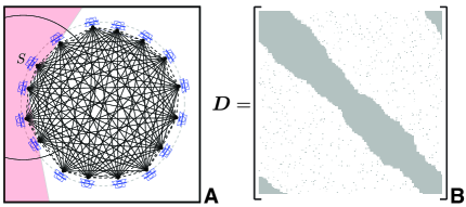
Figure 4: (A) Ultrasound transducers lie on an approximately circular ring. The ring surrounds the breast and after each transducer fires an ultrasonic signal, the sound speed distribution of the breast is estimated. A precise knowledge of the sensor locations is needed to have an accurate reconstruction of the enclosed medium. (B) Because of the limited beam width of the transducers, noise and imperfect TOF estimation methods, the measured EDM is incomplete and noisy. Gray areas show missing entries of the matrix.

III-B Multidimensional Scaling

Multidimensional scaling refers to a group of techniques that, given a set of noisy distances, find the best fitting point conformation. It was originally proposed in psychometrics [15, 8] to visualize the (dis-)similarities between objects. Initially, MDS was defined as the problem of representing distance data, but now the term is commonly used to refer to methods for solving the problem [39].

Various cost functions were proposed for solving MDS. In Section II-B, we already encountered one method: the classical MDS. This method minimizes the Frobenius norm of the difference between the input matrix and the Gram matrix of the points in the target embedding dimension.

The Gram matrix contains inner products; rather than with inner products, it is better to directly work with the distances. A typical cost function represents the dissimilarity of the observed distances and the distances between the estimated point locations. An essential observation is that the feasible set for these optimizations is not convex (EDMs with embedding dimensions smaller than $n-1$ lie on the boundary of a cone [20], which is a non-convex set).

A popular dissimilarity measure is raw stress [40], defined as the value of

$$\underset{\bm{X}\in\mathbb{R}^{d\times n}}{\text{minimize}} \sum_{(i,j)\in E}\left(\sqrt{\mathrm{edm}(\bm{X})_{ij}}-\sqrt{\widetilde{d}_{ij}}\right)^{2}\,,$$ (24)

where $E$ defines the set of revealed elements of the distance matrix $\bm{D}$. The objective function can be concisely written as $\big{\|}\bm{W}\circ\big{(}\sqrt{\mathrm{edm}(\bm{X})}-\sqrt{\widetilde{\bm{D}}}\big{)}\big{\|}_{F}^{2}$; a drawback of this cost function is that it is not globally differentiable. Approaches described in the literature comprise iterative majorization [41], various methods using convex analysis [42] and steepest descent methods [43].

Another well-known cost function is s-stress,

$$\underset{\bm{X}\in\mathbb{R}^{d\times n}}{\text{minimize}} \sum_{(i,j)\in E}\left(\mathrm{edm}(\bm{X})_{ij}-\widetilde{d}_{ij}\right)^{2}\,.$$ (25)

Again, we write the objective concisely as $\big{\|}\bm{W}\circ\big{(}\mathrm{edm}(\bm{X})-\widetilde{\bm{D}}\big{)}\big{\|}_{F}^{2}$. It was first studied by Takane, Young and De Leeuw [44]. Conveniently, the s-stress objective is everywhere differentiable, but at a disadvantage that it favors large over small distances. Gaffke and Mathar [45] propose an algorithm to find the global minimum of the s-stress function for embedding dimension $d=n-1$. EDMs with this embedding dimension exceptionally constitute a convex set [20], but we are typically interested in embedding dimensions much smaller than $n$. The s-stress minimization in (25) is not convex for $d<n-1$. It was analytically shown to have saddle points [46], but interestingly, no analytical non-global minimizer has been found [46].

Browne proposed a method for computing s-stress based on Newton-Raphson root finding [47]. Glunt reports that the method by Browne converges to the global minimum of (25) in 90% of the test cases in his dataset [48].

The cost function in (25) is separable across points $i$ and across coordinates $k$, which is convenient for distributed implementations. Parhizkar [46] proposed an alternating coordinate descent method that leverages this separability, by updating a single coordinate of a particular point at a time. The s-stress function restricted to the $k$th coordinate of the $i$th point is a fourth-order polynomial,

$$f(x;\bm{\alpha}^{(i,k)})=\sum_{\ell=0}^{4}\alpha_{\ell}^{(i,k)}x^{\ell},$$ (26)

where $\bm{\alpha}^{(i,k)}$ lists the polynomial coefficients for $i$th point and $k$th coordinate. For example, $\alpha^{(i,k)}_{0}=4\sum_{j}w_{ij}$, that is, four times the number of points connected to point $i$. Expressions for the remaining coefficients are given in [46]; in the pseudocode (Algorithm 4), we assume that these coefficients are returned by the function “GetQuadricCoeffs”, given the noisy incomplete matrix $\widetilde{\bm{D}}$, the observation mask $\bm{W}$ and the dimensionality $d$. The global minimizer of (26) can be found analytically by calculating the roots of its derivative (a cubic). The process is then repeated over all coordinates $k$, and points $i$, until convergence. The resulting algorithm is remarkably simple, yet empirically converges fast. It naturally lends itself to a distributed implementation. We spell it out in Algorithm 4.

When applied to a large dataset of random, noiseless and complete distance matrices, Algorithm 4 converges to the global minimum of (25) in more than 99% of the cases [46].

Algorithm 4 Alternating Descent [46]

• function AlternatingDescent($\widetilde{\bm{D}},\bm{W},d$)

• $\bm{X}\in\mathbb{R}^{d\times n}\leftarrow\bm{X}_{0}=\bm{\mathit{0}}$ $\triangleright$ Initialize the point set

• repeat

• for $i\in\{1,\cdots,n\}$ do $\triangleright$ Points

• for $k\in\{1,\cdots,d\}$ do $\triangleright$ Coordinates

• $\bm{\alpha}^{(i,k)}\leftarrow\text{GetQuadricCoeffs}(\bm{W},\widetilde{\bm{D}},d)$

• $x_{i,k}\leftarrow\operatorname*{arg\,min}_{x}f(x;\bm{\alpha}^{(i,k)})$ $\triangleright$ Eq. (26)

• end for

• end for

• until Convergence or MaxIter

• return $\bm{X}$

• end function

III-C Semidefinite Programming

Recall the characterization of EDMs (11) in Theorem 2. It states that $\bm{D}$ is an EDM if and only if the corresponding geometrically centered Gram matrix $-\frac{1}{2}\bm{J}\bm{D}\bm{J}$ is positive-semidefinite. Thus, it establishes a one-to-one correspondence between the cone of EDMs, denoted by $\mathbb{EDM}^{n}$, and the intersection of the symmetric positive-semidefinite cone $\mathbb{S}_{+}^{n}$ with the geometrically centered cone $\mathbb{S}_{c}^{n}$. The latter is defined as the set of all symmetric matrices whose column sum vanishes,

$$\mathbb{S}_{c}^{n}=\left\{\bm{G}\in\mathbb{R}^{n\times n}\ |\ \bm{G}=\bm{G}^{\top},\ \bm{G}\bm{\mathit{1}}=\bm{\mathit{0}}\right\}.$$ (27)

We can use this correspondence to cast EDM completion and approximation as semidefinite programs. While (11) describes an EDM of an $n$-point configuration in any dimension, we are often interested in situations where $d\ll n$. It is easy to adjust for this case by requiring that the rank of the centered Gram matrix be bounded. One can verify that

$$\begin{rcases*}\bm{D}=\mathrm{edm}(\bm{X})\\ \mathrm{affdim}(\bm{X})\leq d\end{rcases*}\quad\Longleftrightarrow\quad\begin{cases}-\frac{1}{2}\bm{J}\bm{D}\bm{J}\succeq 0\\ \mathop{\mathrm{rank}}(\bm{J}\bm{D}\bm{J})\leq d,\end{cases}$$ (28)

when $n\geq d$. That is, EDMs with a particular embedding dimension $d$ are completely characterized by the rank and definiteness of $\bm{J}\bm{D}\bm{J}$.

Now we can write the following rank-constrained semidefinite program for solving Problem 1,

$$\underset{\bm{G}}{\text{minimize}} \left\lVert\bm{W}\circ\left(\widetilde{\bm{D}}-\mathcal{K}(\bm{G})\right)\right\rVert_{F}^{2}$$ (29)

subject to $$\mathop{\mathrm{rank}}(\bm{G})\leq d$$

$$\bm{G}\in\mathbb{S}^{n}_{+}\cap\mathbb{S}^{n}_{c}.$$

The second constraint is just a shorthand for writing $\bm{G}\succeq 0,\ \bm{G}\bm{\mathit{1}}=\bm{\mathit{0}}$. We note that this is equivalent to MDS with the s-stress cost function, thanks to the rank characterization (28).

Unfortunately, the rank property makes the feasible set in (29) non-convex, and solving it exactly becomes difficult. This makes sense, as we know that s-stress is not convex. Nevertheless, we may relax the hard problem, by simply omitting the rank constraint, and hope to obtain a solution with the correct dimensionality,

$$\underset{\bm{G}}{\text{minimize}} \left\lVert\bm{W}\circ\left(\widetilde{\bm{D}}-\mathcal{K}(\bm{G})\right)\right\rVert_{F}^{2}$$ (30)

subject to $$\bm{G}\in\mathbb{S}^{n}_{+}\cap\mathbb{S}^{n}_{c}.$$

We call (30) a semidefinite relaxation (SDR) of the rank-constrained program (29).

The constraint $\bm{G}\in\mathbb{S}_{c}^{n}$, or equivalently, $\bm{G}\bm{\mathit{1}}=\bm{\mathit{0}}$, means that there are no strictly positive definite solutions ($\bm{G}$ has a nullspace, so at least one eigenvalue must be zero). In other words, there exist no strictly feasible points [32]. This may pose a numerical problem, especially for various interior point methods. The idea is then to reduce the size of the Gram matrix through an invertible transformation, somehow removing the part of it responsible for the nullspace. In what follows, we describe how to construct this smaller Gram matrix.

A different, equivalent way to phrase the multiplicative characterization (11) is the following statement: a symmetric hollow matrix $\bm{D}$ is an EDM if and only if it is negative semidefinite on $\left\{\bm{\mathit{1}}\right\}^{\perp}$ (on all vectors $\bm{t}$ such that $\bm{t}^{\top}\bm{\mathit{1}}=0$). Let us construct an orthonormal basis for this orthogonal complement—a subspace of dimension $(n-1)$—and arrange it in the columns of matrix $\bm{V}\in\mathbb{R}^{n\times(n-1)}$. We demand

$$\bm{V}^{\top}\bm{\mathit{1}}=\bm{\mathit{0}}$$ (31)

$$\bm{V}^{\top}\bm{V}=\bm{I}.$$

There are many possible choices for $\bm{V}$, but all of them obey that $\bm{V}\bm{V}^{\top}=\bm{I}-\frac{1}{n}\bm{\mathit{1}}\bm{\mathit{1}}^{\top}=\bm{J}$. The following choice is given in [2],

$$\bm{V}=\begin{bmatrix}p&p&\cdots&p\\ 1+q&q&\cdots&q\\ q&1+q&\cdots&q\\ \vdots&\cdots&\ddots&\vdots\\ q&q&\cdots&1+q\end{bmatrix},$$ (32)

where $p=-1/(n+\sqrt{n})$ and $q=-1/\sqrt{n}$.

With the help of the matrix $\bm{V}$, we can now construct the sought Gramian with reduced dimensions. For an EDM $\bm{D}\in\mathbb{R}^{n\times n}$,

$$\mathcal{G}(\bm{D})\overset{\text{def}}{=}-\frac{1}{2}\bm{V}^{\top}\bm{D}\bm{V}$$ (33)

is an $(n-1)\times(n-1)$ PSD matrix. This can be verified by substituting (33) in (4). Additionally, we have that

$$\mathcal{K}(\bm{V}\mathcal{G}(\bm{D})\bm{V}^{\top})=\bm{D}.$$ (34)

Indeed, $\bm{H}\mapsto\mathcal{K}(\bm{V}\bm{H}\bm{V}^{\top})$ is an invertible mapping from $\bm{S}_{+}^{n-1}$ to $\mathbb{EDM}^{n}$ whose inverse is exactly $\mathcal{\bm{G}}$. Using these notations we can write down an equivalent optimization program that is numerically more stable than (30) [2]:

$$\underset{\bm{H}}{\text{minimize}} \left\lVert\bm{W}\circ\left(\widetilde{\bm{D}}-\mathcal{K}(\bm{V}\bm{H}\bm{V}^{\top})\right)\right\rVert_{F}^{2}$$ (35)

subject to $$\bm{H}\in\mathbb{S}^{n-1}_{+}.$$

On the one hand, with the above transformation the constraint $\bm{G}\bm{\mathit{1}}=\bm{\mathit{0}}$ became implicit in the objective, as $\bm{V}\bm{H}\bm{V}^{\top}\bm{\mathit{1}}\equiv\bm{\mathit{0}}$ by (31); on the other hand, the feasible set is now the full semidefinite cone $\mathbb{S}_{+}^{n-1}$.

Still, as Krislock & Wolkowicz mention [32], by omitting the rank constraint we allow the points to move about in a larger space, so we may end up with a higher-dimensional solution even if there is a completion in dimension $d$.

There exist various heuristics for promoting lower rank. One such heuristic involves the trace norm—the convex envelope of rank. The trace or nuclear norm is studied extensively by the compressed sensing community. In contrast to the common wisdom in compressed sensing, the trick here is to maximize the trace norm, not to minimize it. The mechanics are as follows: maximizing the sum of squared distances between the points will stretch the configuration as much as possible, subject to available constraints. But stretching favors smaller affine dimensions (imagine pulling out a roll of paper, or stretching a bent string). Maximizing the sum of squared distances can be rewritten as maximizing the sum of norms in a centered point configuration—but that is exactly the trace of the Gram matrix $\bm{G}=-\frac{1}{2}\bm{J}\bm{D}\bm{J}$ [9]. This idea has been successfully put to work by Weinberger and Saul [9] in manifold learning, and by Biswas et al. in SNL [49].

Algorithm 5 Semidefinite Relaxation (Matlab/CVX)

⬇

1ction [EDM, X] = sdr_complete_edm(D, W, lambda)

2

3n = size(D, 1);

4x = -1/(n + sqrt(n));

5y = -1/sqrt(n);

6V = [y*ones(1, n-1); x*ones(n-1) + eye(n-1)];

7e = ones(n, 1);

8

9cvx_begin sdp

10 variable G(n-1, n-1) symmetric;

11 B = V*G*V';

12 E = diag(B)*e' + e*diag(B)' - 2*B;

13 maximize trace(G) ...

14 - lambda * norm(W .* (E - D), 'fro');

15 subject to

16 G >= 0;

17cvx_end

18

19[U, S, V] = svd(B);

20EDM = diag(B)*e' + e*diag(B)' - 2*B;

21X = sqrt(S)*V';

Noting that $\mathop{\mathrm{trace}}(\bm{H})=\mathop{\mathrm{trace}}(\bm{G})$ because $\mathop{\mathrm{trace}}(\bm{J}\bm{D}\bm{J})=\mathop{\mathrm{trace}}(\bm{V}^{\top}\bm{D}\bm{V})$, we write the following SDR,

$$\underset{\bm{H}}{\text{maximize}} \mathop{\mathrm{trace}}(\bm{H})-\lambda\left\lVert\bm{W}\circ\big{(}\widetilde{\bm{D}}-\mathcal{K}(\bm{V}\bm{H}\bm{V}^{\top})\big{)}\right\rVert_{F}$$

subject to $$\bm{H}\in\mathbb{S}^{n-1}_{+}$$ (36)

Here we opted to include the data fidelity term in the Lagrangian form, as proposed by Biswas [49], but it could also be moved to constraints. Finally, in all of the above relaxations, it is straightforward to include upper and lower bounds on the distances. Because the bounds are linear constraints, the resulting programs remain convex; this is particularly useful in the molecular conformation problem. A Matlab/CVX [50, 51] implementation of the SDR (III-C) is given in Algorithm 5.

III-D Multidimensional Unfolding: A Special Case of Completion

Figure 5: Microphone calibration as an example of MDU. We can measure only the propagation times from acoustic sources at unknown locations, to microphones at unknown locations. The corresponding revealed part of the EDM has a particular off-diagonal structure, leading to a special case of EDM completion.

Imagine that we partition the point set into two subsets, and that we can measure the distances between the points belonging to different subsets, but not between the points in the same subset. Metric multidimensional unfolding (MDU) [30] refers to this special case of EDM completion.

MDU is relevant for position calibration of ad-hoc sensor networks, in particular of microphones. Consider an ad-hoc array of $m$ microphones at unknown locations. We can measure the distances to $k$ point sources, also at unknown locations, for example by emitting a pulse (we assume that the sources and the microphones are synchronized). We can always permute the points so that the matrix assumes the structure shown in Fig. 5, with the unknown entries in two diagonal blocks. This is a standard scenario described for example in [27].

One of the early approaches to metric MDU is that of Schönemann [30]. We go through the steps of the algorithm, and then explain how to solve the problem using the EDM toolbox. The goal is to make a comparison, and emphasize the universality and simplicity of the introduced tools.

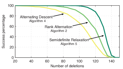
Figure 6: Comparison of different algorithms applied to completing an EDM with random deletions. For every number of deletions, we generated 2000 realizations of 20 points uniformly at random in a unit square. Distances to delete were chosen uniformly at random among the resulting $\binom{20}{2}=190$ pairs; 20 deletions correspond to $\approx$ 10% of the number of distance pairs and to 5% of the number of matrix entries; 150 deletions correspond to $\approx$ 80% of the distance pairs and to $\approx$ 38% of the number of matrix entries. Success was declared if the Frobenius norm of the error between the estimated matrix and the true EDM was less than 1% of the Frobenius norm of the true EDM.

Denote by $\bm{R}=[\bm{r}_{1},\ \ldots,\ \bm{r}_{m}]$ the unknown microphone locations, and by $\bm{S}=[\bm{s}_{1},\ \ldots,\ \bm{s}_{k}]$ the unknown source locations. The distance between the $i$th microphone and $j$th source is

$$\delta_{ij}=\left\lVert\bm{r}_{i}-\bm{s}_{j}\right\rVert^{2},$$ (37)

so that in analogy with (3) we have

$$\bm{\mathit{\Delta}}=\mathrm{edm}(\bm{R},\bm{S})=\mathop{\mathrm{diag}}(\bm{R}^{\top}\bm{R})\bm{\mathit{1}}^{\top}-2\bm{R}^{\top}\bm{S}+\bm{\mathit{1}}\mathop{\mathrm{diag}}(\bm{S}^{\top}\bm{S}),$$ (38)

where we overloaded the $\mathrm{edm}$ operator in a natural way. We use $\bm{\mathit{\Delta}}$ to avoid confusion with the standard Euclidean $\bm{D}$. Consider now two geometric centering matrices of sizes $m$ and $k$, denoted $\bm{J}_{m}$ and $\bm{J}_{k}$. Similarly to (14), we have

$$\bm{R}\bm{J}_{m}=\bm{R}-\bm{r}_{c}\bm{\mathit{1}}^{\top},\ \bm{S}\bm{J}_{k}=\bm{S}-\bm{s}_{c}\bm{\mathit{1}}^{\top}.$$ (39)

This means that

$$\bm{J}_{m}\bm{\mathit{\Delta}}\bm{J}_{k}=\widetilde{\bm{R}}^{\top}\widetilde{\bm{S}}\overset{\text{def}}{=}\widetilde{\bm{G}}$$ (40)

is a matrix of inner products between vectors $\widetilde{\bm{r}}_{i}$ and $\widetilde{\bm{s}}_{j}$. We used tildes to differentiate this from real inner products betwen $\bm{r}_{i}$ and $\bm{s}_{j}$, because in (40), the points in $\widetilde{\bm{R}}$ and $\widetilde{\bm{S}}$ are referenced to different coordinate systems. The centroids $\bm{r}_{c}$ and $\bm{s}_{c}$ generally do not coincide. There are different ways to decompose $\widetilde{\bm{G}}$ into a product of two full rank matrices, call them $\bm{A}$ and $\bm{B}$,

$$\widetilde{\bm{G}}=\bm{A}^{\top}\bm{B}.$$ (41)

We could for example use the SVD, $\widetilde{\bm{G}}=\bm{U}\bm{\Sigma}\bm{V}^{\top}$, and set $\bm{A}^{\top}=\bm{U}$ and $\bm{B}=\bm{\Sigma}\bm{V}^{\top}$. Any two such decompositions are linked by some invertible transformation $\bm{T}\in\mathbb{R}^{d\times d}$,

$$\widetilde{\bm{G}}=\bm{A}^{\top}\bm{B}=\widetilde{\bm{R}}^{\top}\bm{T}^{-1}\bm{T}\widetilde{\bm{S}}.$$ (42)

We can now write down the conversion rule from what we can measure to what we can compute,

$$\bm{R}=\bm{T}^{\top}\bm{A}+\bm{r}_{c}\bm{\mathit{1}}^{\top}$$ (43)

$$\bm{S}=(\bm{T}^{-1})^{\top}\bm{B}+\bm{s}_{c}\bm{\mathit{1}}^{\top},$$

where $\bm{A}$ and $\bm{B}$ can be computed according to (41). Because we cannot reconstruct the absolute position of the point set, we can arbitrarily set $\bm{r}_{c}=0$, and $\bm{s}_{c}=\alpha\bm{e}_{1}$. Recapitulating, we have that

$$\bm{\mathit{\Delta}}=\mathrm{edm}\left(\bm{T}^{\top}\!\bm{A},\ (\bm{T}^{-1})^{\top}\bm{B}+\alpha\bm{e}_{1}\bm{\mathit{1}}^{\top}\right),$$ (44)

and the problem is reduced to computing $\bm{T}$ and $\alpha$ so that (44) hold, or in other words, so that the right hand side be consistent with the data $\bm{\mathit{\Delta}}$. We reduced MDU to a relatively small problem: in 3D, we need to compute only ten scalars. Schönemann [30] gives an algebraic method to find these parameters, and mentions the possibility of least squares, while Crocco, Bue and Murino [27] propose a different approach using non-linear least squares.

This procedure seems quite convoluted. Rather, we see MDU as a special case of matrix completion, with the structure illustrated in Fig. 5.

More concretely, represent the microphones and the sources by a set of $n=k+m$ points, ascribed to the columns of matrix $\bm{X}=[\bm{R}\ \bm{S}]$. Then $\mathrm{edm}(\bm{X})$ has a special structure as seen in Fig. 5,

$$\mathrm{edm}(\bm{X})=\begin{bmatrix}\mathrm{edm}(\bm{R})&\mathrm{edm}(\bm{R},\bm{S})\\ \mathrm{edm}(\bm{S},\bm{R})&\mathrm{edm}(\bm{S})\end{bmatrix}.$$ (45)

We define the mask matrix for MDU as

$$\bm{W}_{\text{MDU}}\overset{\text{def}}{=}\begin{bmatrix}\bm{\mathit{0}}_{m\times m}&\bm{\mathit{1}}_{m\times k}\\ \bm{\mathit{1}}_{k\times m}&\bm{\mathit{0}}_{k\times k}\end{bmatrix}.$$ (46)

With this matrix, we can simply invoke the SDR in Algorithm 5. We could also use Algorithm 2, or Algorithm 4. Performance of different algorithms is compared in Section III-E.

It is worth mentioning that SNL specific algorithms that exploit the particular graph induced by limited range communication do not perform well on MDU. This is because the structure of the missing entries in MDU is in a certain sense opposite to the one of SNL.

III-E Performance Comparison of Algorithms

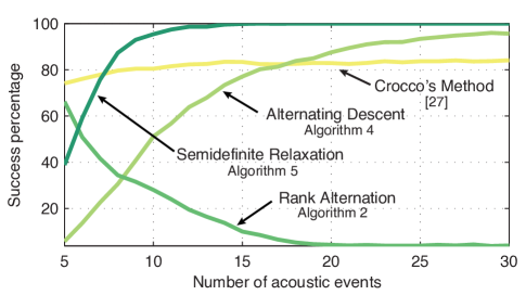
Figure 7: Comparison of different algorithms applied to multidimensional unfolding with varying number of acoustic events $k$. For every number of acoustic events, we generated 3000 realizations of $m=20$ microphone locations uniformly at random in a unit cube. Percentage of missing matrix entries is given as $(k^{2}+m^{2})/(k+m)^{2}$, so that the ticks on the abscissa correspond to $[68,56,51,50,51,52]\%$ (non-monotonic in $k$ with the minimum for $k=m=20$). Success was declared if the Frobenius norm of the error between the estimated matrix and the true EDM was less than 1% of the Frobenius norm of the true EDM.

We compare the described algorithms in two different EDM completion settings. In the first experiment (Figs. 6 and 8), the entries to delete are chosen uniformly at random. The second experiment (Figs. 7 and 9) tests performance in MDU, where the non-observed entries are highly structured. In Figs. 6 and 7, we assume that the observed entries are known exactly, and we plot the success rate (percentage of accurate EDM reconstructions) against the number of deletions in the first case, and the number of calibration events in the second case. Accurate reconstruction is defined in terms of the relative error. Let $\bm{D}$ be the true, and $\widehat{\bm{D}}$ the estimated EDM. The relative error is then ${\|\widehat{\bm{D}}-\bm{D}\|_{F}}/{\|\bm{D}\|_{F}}$, and we declare success if this error is below $1\%$.

To generate Figs. 8 and 9 we varied the amount of random, uniformly distributed jitter added to the distances, and for each jitter level we plotted the relative error. The exact values of intermediate curves are less important than the curves for the smallest and the largest jitter, and the overall shape of the ensemble.

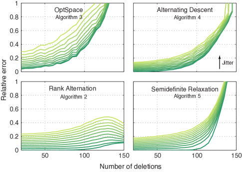
Figure 8: Comparison of different algorithms applied to completing an EDM with random deletions and noisy distances. For every number of deletions, we generated 1000 realizations of 20 points uniformly at random in a unit square. In addition to the number of deletions, we varied the amount of jitter added to the distances. Jitter was drawn from a centered uniform distribution, with the level increasing in the direction of the arrow, from $\mathcal{U}[0,0]$ (no jitter) for the darkest curve at the bottom, to $\mathcal{U}[-0.15,0.15]$ for the lightest curve at the top, in 11 increments. For every jitter level, we plotted the mean relative error $\|\widehat{\bm{D}}-\bm{D}\|_{F}/\|\bm{D}\|_{F}$ for all algorithms.

A number of observations can be made about the performance of algorithms. Notably, OptSpace (Algorithm 3) does not perform well for randomly deleted entries when $n=20$; it was designed for larger matrices. For this matrix size, the mean relative reconstruction error achieved by OptSpace is the worst of all algorithms (Fig. 8). In fact, the relative error in the noiseless case was rarely below the success threshold (set to $1\%$) so we omitted the corresponding near-zero curve from Fig. 6. Furthermore, OptSpace assumes that the pattern of missing entries is random; in the case of a blocked deterministic structure associated with MDU, it never yields a satisfactory completion.

On the other hand, when the unobserved entries are randomly scattered in the matrix, and the matrix is large—in the ultrasonic calibration example the number of sensors $n$ was $200$ or more—OptSpace is a very fast and attractive algorithm. To fully exploit OptSpace, $n$ should be even larger, in the thousands or tens of thousands.

SDR (Algorithm 5) performs well in all scenarios. For both the random deletions and the MDU, it has the highest success rate, and it behaves well with respect to noise. Alternating coordinate descent (Algorithm 4) performs slightly better in noise for small number of deletions and large number of calibration events, but Figs. 6 and 7 indicate that for certain realizations of the point set it gives large errors. If the worst-case performance is critical, SDR is a better choice. We note that in the experiments involving the SDR, we have set the multiplier $\lambda$ in III-C to the square root of the number of missing entries. This choice was empirically found to perform well.

The main drawback of SDR is speed; it is the slowest among the tested algorithms. To solve the semidefinite program we used CVX [50, 51], a Matlab interface to various interior point methods. For larger matrices (e.g., $n=1000$), CVX runs out of memory on a desktop computer, and essentially never finishes. Matlab implementations of alternating coordinate descent, rank alternation (Algorithm 2), and OptSpace are all much faster.

The microphone calibration algorithm by Crocco [27] performs equally well for any number of acoustic events. This may be explained by the fact that it always reduces the problem to ten unknowns. It is an attractive choice for practical calibration problems with a smaller number of calibration events. Algorithm’s success rate can be further improved if one is prepared to run it for many random initializations of the non-linear optimization step.

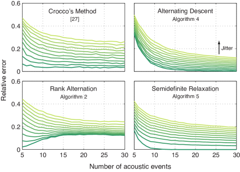
Figure 9: Comparison of different algorithms applied to multidimensional unfolding with varying number of acoustic events $k$ and noisy distances. For every number of acoustic events, we generated 1000 realizations of $m=20$ microphone locations uniformly at random in a unit cube. In addition to the number of acoustic events, we varied the amount of random jitter added to the distances, with the same parameters as in Fig. 8. For every jitter level, we plotted the mean relative error $\|\widehat{\bm{D}}-\bm{D}\|_{F}/\|\bm{D}\|_{F}$ for all algorithms.

Interesting behavior can be observed for the rank alternation in MDU. Figs. 7 and 9 both show that at low noise levels, the performance of the rank alternation becomes worse with the number of acoustic events. At first glance, this may seem counterintuitive, as more acoustic events means more information; one could simply ignore some of them, and perform at least equally well as with fewer events. But this reasoning presumes that the method is aware of the geometrical meaning of the matrix entries; on the contrary, rank alternation is using only rank. Therefore, even if the percentage of the observed matrix entries grows until a certain point, the size of the structured blocks of unknown entries grows as well (and the percentage of known entries in columns/rows corresponding to acoustic events decreases). This makes it harder for a method that does not use geometric relationships to complete the matrix. A loose comparison can be made to image inpainting: If the pixels are missing randomly, many methods will do a good job; but if a large patch is missing, we cannot do much without additional structure (in our case geometry), no matter how large the rest of the image is.

To summarize, for smaller matrices the SDR seems to be the best overall choice. For large matrices the SDR becomes too slow and one should turn to alternating coordinate descent, rank alternation or OptSpace. Rank alternation is the simplest algorithm, but alternating coordinate descent performs better. For very large matrices ($n$ on the order of thousands or tens of thousands), OptSpace becomes the most attractive solution. We note that we deliberately refrained from making detailed running time comparisons, due to the diverse implementations of the algorithms.

III-F Summary

In this section we discussed:

• The problem statement for EDM completion and denoising, and how to easily exploit the rank property (Algorithm 2),

• Standard objective functions in MDS: raw stress and s-stress, and a simple algorithm to minimize s-stress (Algorithm 4),

• Different semidefinite relaxations that exploit the connection between EDMs and PSD matrices,

• Multidimensional unfolding, and how to solve it efficiently using EDM completion,

• Performance of the introduced algorithms in two very different scenarios: EDM completion with randomly unobserved entries, and EDM completion with deterministic block structure of unobserved entries (MDU).

IV Unlabeled Distances

In certain applications we can measure the distances between the points, but we do not know the correct labeling. That is, we know all the entries of an EDM, but we do not know how to arrange them in the matrix. As illustrated in Fig. 10A, we can imagine having a set of sticks of various lengths. The task is to work out the correct way to connect the ends of different sticks so that no stick is left hanging open-ended.

In this section we exploit the fact that in many cases, distance labeling is not essential. For most point configurations, there is no other set of points that can generate the corresponding set of distances, up to a rigid transformation.

Localization from unlabeled distances is relevant in various calibration scenarios where we cannot tell apart distance measurements belonging to different points in space. This can occur when we measure times of arrivals of echoes, which correspond to distances between the microphones and the image sources (see Fig. 12) [29, 6]. Somewhat surprisingly, the same problem of unlabeled distances appears in sparse phase retrieval; to see how, take a look at the “Phase Retrieval” box.

No efficient algorithm currently exists for localization from unlabeled distances in the general case of noisy distances. We should mention, however, a recent polynomial-time algorithm (albeit of a high degree) by Gujarathi and et al. [31], that can reconstruct relatively large point sets from unordered, noiseless distance data.

At any rate, the number of assignments to test is sometimes sufficiently small so that an exhaustive search does not present a problem. We can then use EDMs to find the best labeling. The key to the unknown permutation problem is the following fact.

Theorem 3.

Draw $\bm{x}_{1},\bm{x}_{2},\cdots,\bm{x}_{n}\in\mathbb{R}^{d}$ independently from some absolutely continuous probability distribution (e.g. uniformly at random) on $\Omega\subseteq\mathbb{R}^{d}$. Then with probability 1, the obtained point configuration is the unique (up to a rigid transformation) point configuration in $\Omega$ that generates the set of distances $\left\{\left\lVert\bm{x}_{i}-\bm{x}_{j}\right\rVert,1\leq i<j\leq n\right\}$.

This fact is a simple consequence of a result by Boutin and Kemper [52] who give a characterization of point sets reconstructible from unlabeled distances.

Figs. 10B and 10C show two possible arrangements of the set of distances in a tentative EDM; the only difference is that the two hatched entries are swapped. But this simple swap is not harmless: there is no way to attach the last stick in Fig. 10D, while keeping the remaining triangles consistent. We could do it in a higher embedding dimension, but we insist on realizing it in the plane.

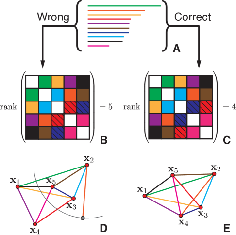
Figure 10: Illustration of the uniqueness of EDMs for unlabeled distances. A set of unlabeled distance (A) is distributed in two different ways in a tentative EDM with embedding dimension 2 (B and C). The correct assignment yields the matrix with the expected rank (C), and the point set is easily realized in the plane (E). On the contrary, swapping just two distances (hatched squares in (B) and (C)) makes it impossible to realize the point set in the plane (D). Triangles that do not coincide with the swapped edges can still be placed, but in the end we are left with a hanging orange stick that cannot attach itself to any of the five nodes.

What Theorem 3 does not tell us is how to identify the correct labeling. But we know that for most sets of distances, only one (correct!) permutation can be realized in the given embedding dimension. Of course, if all the labelings are unknown and we have no good heuristics to trim the solution space, finding the correct labeling is difficult, as noted in [31]. Yet there are interesting situations where this search is feasible because we can augment the EDM point by point. We describe one such situation in the next subsection.

EDM Perspective on Sparse Phase Retrieval (The Unexpected Distance Structure)

In many cases, it is easier to measure a signal in the Fourier domain. Unfortunately, it is common in these scenarios that we can only reliably measure the magnitude of the Fourier transform (FT). We would like to recover the signal of interest from just the magnitude of its FT, hence the name phase retrieval. X-ray crystallography [54] and speckle imaging in astronomy [55] are classic examples of phase retrieval problems. In both of these applications the signal is spatially sparse. We can model it as

$$f(\bm{x})=\sum_{i=1}^{n}c_{i}\delta(\bm{x}-\bm{x}_{i}),$$ (47)

where $c_{i}$ are the amplitudes and $\bm{x}_{i}$ the locations of the $n$ Dirac deltas in the signal. In what follows, we discuss the problem on 1-dimensional domains, that is $\bm{x}\in\mathbb{R}$, knowing that a multidimensional phase retrieval problem can be solved by solving many 1-dimensional problems [7].

Note that measuring the magnitude of the FT of $f(\bm{x})$ is equivalent to measuring its autocorrelation function (ACF). For a sparse $f(\bm{x})$, the ACF is also sparse and given as

$$a(\bm{x})=\sum_{i=1}^{n}\sum_{j=1}^{n}c_{i}c_{j}\delta(\bm{x}-(\bm{x}_{i}-\bm{x}_{j})),$$ (48)

where we note the presence of differences between the locations $\bm{x}_{i}$ in the support of the ACF. As $a(\bm{x})$ is symmetric, we do not know the order of $\bm{x}_{i}$, and so we can only know these differences up to a sign, which is equivalent to knowing the distances $\left\lVert\bm{x}_{i}-\bm{x}_{j}\right\rVert$.

For the following reasons, we focus on the recovery of the support of the signal $f(\bm{x})$ from the support of the ACF $a(\bm{x})$: i) in certain applications, the amplitudes $c_{i}$ may be all equal, thus limiting their role in the reconstruction; ii) knowing the support of $f(\bm{x})$ and its ACF is sufficient to exactly recover the signal $f(\bm{x})$ [7].

The recovery of the support of $f(\bm{x})$ from the one of $a(\bm{x})$ corresponds to the localization of a set of $n$ points from their unlabeled distances: we have access to all the pairwise distances but we do not know which pair of points corresponds to any given distance. This can be recognized as an instance of the turnpike problem, whose computational complexity is believed not to be NP-hard but for which no polynomial time algorithm is known [56].

From an EDM perspective, we can design a reconstruction algorithm recovering the support of the signal $f(\bm{x})$ by labeling the distances obtained from the ACF such that the resulting EDM has rank smaller or equal than 3. This can be regarded as unidimensional scaling with unlabeled distances, and the algorithm to solve it is similar to echo sorting (Algorithm 6).

Figure 11: A graphical representation of the phase retrieval problem for 1-dimensional sparse signals. (A) We measure the ACF of the signal and we recover a set of distances (sticks in Fig. 10) from its support. (B) These are the unlabeled distances between all the pairs of Dirac deltas in the signal $f(\bm{x})$. We exactly recover the support of the signal if we correctly label the distances.

IV-A Hearing the Shape of a Room [6]

An important application of EDMs with unlabeled distances is the reconstruction of the room shape from echoes. An acoustic setup is shown in Fig. 12A, but one could also use radio signals. Microphones pick up the convolution of the sound emitted by the loudspeaker with the room impulse response (RIR), which can be estimated by knowing the emitted sound. An example RIR recorded by one of the microphones is illustrated in Fig. 12B, with peaks highlighted in green. Some of these peaks are first-order echoes coming from different walls, and some are higher-order echoes or just noise.

Echoes are linked to the room geometry by the image source model [53]. According to this model, we can replace echoes by image sources (IS)—mirror images of the true sources across the corresponding walls. Position of the image source of $\bm{s}$ corresponding to wall $i$ is computed as

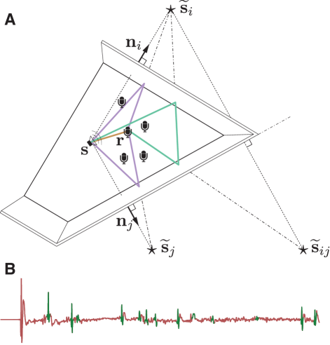
Figure 12: (A) Illustration of the image source model for first- and second-order echoes. Vector $\bm{n}_{i}$ is the outward-pointing unit normal associated with the $i$th wall. Stars denote the image sources, and $\widetilde{\bm{s}}_{ij}$ is the image source corresponding to the second-order echo. Sound rays corresponding to first reflections are shown in blue, and the ray corresponding to the second-order reflection is shown in red. (B) Early part of a typical recorded room impulse response.

$$\widetilde{\bm{s}}_{i}=\bm{s}+2\left\langle\bm{p}_{i}-\bm{s},\bm{n}_{i}\right\rangle\bm{n}_{i},$$ (49)

where $\bm{p}_{i}$ is any point on the $i$th wall, and $\bm{n}_{i}$ is the unit normal vector associated with the $i$th wall, see Fig. 12A. A convex room with planar walls is completely determined by the locations of first-order ISs [6], so by reconstructing their locations, we actually reconstruct the room’s geometry.

We assume that the loudspeaker and the microphones are synchronized so that the times at which the echoes arrive directly correspond to distances. The challenge is that the distances—the green peaks in Fig. 12B—are unlabeled: it might happen that the $k$th peak in the RIR from microphone 1 and the $k$th peak in the RIR from microphone 2 come from different walls, especially for larger microphone arrays. Thus, we have to address the problem of echo sorting, in order to group peaks corresponding to the same image source in RIRs from different microphones.

Assuming that we know the pairwise distances between the microphones $\bm{R}=[\bm{r}_{1},\ldots,\bm{r}_{m}]$, we can create an EDM corresponding to the microphone array. Because echoes correspond to image sources, and image sources are just points in space, we attempt to grow that EDM by adding one point—an image source—at a time. To do that, we pick one echo from every microphone’s impulse response, augment the EDM based on echo arrival times, and check how far the augmented matrix is from an EDM with embedding dimension three, as we work in 3D space. The distance from an EDM is measured with s-stress cost function. It was shown in [6] that a variant of Theorem 3 applies to image sources when microphones are thrown at random. Therefore, if the augmented matrix satisfies the EDM properties, almost surely we have found a good image source. With probability 1, no other combination of points could have generated the used distances.

The main reason for using EDMs and s-stress instead of, for instance, the rank property, is that we get robust algorithms. Echo arrival times are corrupted with various errors, and relying on the rank is too brittle. It was verified experimentally [6] that EDMs and s-stress yield a very robust filter for the correct combinations of echoes.

Thus we may try all feasible combinations of echoes, and expect to get exactly one “good” combination for every image source that is “visible” in the impulse responses. In this case, as we are only adding a single point, the search space is small enough to be rapidly traversed exhaustively. Geometric considerations allow for a further trimming of the search space: because we know the diameter of the microphone array, we know that an echo from a particular wall must arrive at all the microphones within a temporal window corresponding to the array’s diameter.

The procedure is as follows: collect all echo arrival times received by the $i$th microphone in the set $T_{i}$, and fix $t_{1}\in T_{1}$ corresponding to a particular image source. Then Algorithm 6 finds echoes in other microphones’ RIRs that correspond to this same image source. Once we group all the peaks corresponding to one image source, we can determine its location by multilateration (e.g. by running the classical MDS), and then repeat the process for other echoes in $T_{1}$.

To get a ballpark idea of the number of combinations to test, suppose that we detect 20 echoes per microphone, and that the diameter of the five-microphone array is $1.5$ m. Thus for every peak time $t_{1}\in T_{1}$ we have to look for peaks in the remaining four microphones that arrived within a window around $t_{1}$ of length $2\times\frac{1\text{~{}m}}{343\text{~{}m/s}}$, where $343$ m/s is the speed of sound. This is approximately $6$ ms, and in a typical room we can expect about five early echoes within a window of that duration. Thus we have to compute the s-stress for $20\times 5^{4}=12500$ matrices of size $6\times 6$, which can be done in a matter of seconds on a desktop computer. In fact, once we assign an echo to an image source, we can exclude it from further testing, so the number of combinations can be further reduced.

Algorithm 6 Echo Sorting [6]

• function EchoSort($\bm{R},t_{1},\ldots,T_{m}$)

• $\bm{D}\leftarrow\mathrm{edm}(\bm{R})$

• $s_{\mathrm{best}}\leftarrow+\mathrm{Inf}$

• for all $\bm{t}=[t_{2},\ldots,t_{m}],\ \text{such that}~{}t_{i}\in T_{i}$ do

• $\bm{d}\leftarrow c\cdot[t_{1},\ \bm{t}^{\top}]^{\top}$ $\triangleright$ $c$ is the sound speed

• $\bm{D}_{\text{aug}}\leftarrow\begin{bmatrix}\bm{D}&\bm{d}\\ \bm{d}^{\top}&0\end{bmatrix}$

• if $\mathrm{s\!-\!stress}(\bm{D}_{\mathrm{aug}})<s_{\mathrm{best}}$ then

• $s_{\mathrm{best}}\leftarrow\mathrm{s\!-\!stress}(\bm{D}_{\mathrm{aug}})$

• $\bm{d}_{\mathrm{best}}\leftarrow\bm{d}$

• end if

• end for

• return $\bm{d}_{\mathrm{best}}$

• end function

Algorithm 6 was used to reconstruct rooms with centimeter precision [6] with one loudspeaker and an array of five microphones. The same algorithm also enables a dual application: indoor localization of an acoustic source using only one microphone—a feat not possible if we are not in a room [57].

IV-B Summary

To summarize this section:

• We explained that for most point sets, the distances they generate are unique; there are no other point sets generating the same distances,

• In room reconstruction from echoes, we need to identify the correct labeling of the distances to image sources. EDMs act as a robust filter for echoes coming from the same image source,

• Sparse phase retrieval can be cast as a distance problem, too. The support of the ACF gives us distances between the deltas in the original signal. Echo sorting can be adapted to solve the problem from the EDM perspective.

TABLE II: Applications of EDMs with different twists

Application	missing  distances	noisy distances	unlabeled distances
Wireless sensor networks	✔	✔	$\times$
Molecular conformation	✔	✔	$\times$
Hearing the shape of a room	$\times$	✔	✔
Indoor localization	$\times$	✔	✔
Calibration	✔	✔	$\times$
Sparse phase retrieval	$\times$	✔	✔

V Ideas for Future Research

Even problems that at first glance seem to have little to do with EDMs, sometimes reveal a distance structure when you look closely. A good example is sparse phase retrieval.

The purpose of this paper is to convince the reader that Euclidean distance matrices are powerful objects with a multitude of applications (Table II lists various flavors), and that they should belong to any practitioner’s toolbox. We have an impression that the power of EDMs and the associated algorithms has not been sufficiently recognized in the signal processing community, and our goal is to provide a good starting reference. To this end, and perhaps to inspire new research directions, we list several EDM-related problems that we are curious about and believe are important.

Distance matrices on manifolds

If the points lie on a particular manifold, what can be said about their distance matrix? We know that if the points are on a circle, the EDM has rank three instead of four, and this generalizes to hyperspheres [17]. But what about more general manifolds? Are there invertible transforms of the data or of the Gram matrix that yield EDMs with a lower rank than the embedding dimension suggests? What about different distances, e.g. the geodesic distance on the manifold? Answers to these questions have immediate applications in machine learning, where the data can be approximately assumed to be on a smooth surface [23].

Projections of EDMs on lower dimensional subspaces

What happens to an EDM when we project its generating points to a lower dimensional space? What is the minimum number of projections that we need to be able to reconstruct the original point set? Answers to these questions have significant impact on imaging applications such as X-ray crystallography and seismic imaging. What happens when we only have partial distance observations in various subspaces? What are other useful low-dimensional structures on which we can observe the high-dimensional distance data?

Efficient algorithms for distance labeling

Without application-specific heuristics to trim down the search space, identifying correct labeling of the distances quickly becomes an arduous task. Can we identify scenarios for which there are efficient labeling algorithms? What happens when we do not have the labeling, but we also do not have the complete collection of sticks? What can we say about uniqueness of incomplete unlabeled distance sets? Some of the questions have been answered by Gujarathi [31], but many remain. The quest is on for faster algorithms, as well as algorithms that can handle noisy distances.

In particular, if the noise distribution on the unlabeled distances is known, what can we say about the distribution of the reconstructed point set (taking in some sense the best reconstruction over all labelings)? Is it compact, or we can jump to totally wrong assignments with positive probability?

Analytical local minimum of s-stress

Everyone agrees that there are many, but to the best of our knowledge, no analytical minimum of s-stress has yet been found.

VI Conclusion

At the end of this tutorial, we hope that we succeeded in showing how universally useful EDMs are, and that we inspired readers coming across this material for the first time to dig deeper. Distance measurements are so common that a simple, yet sophisticated tool like EDMs deserves attention. A good example is the semidefinite relaxation: even though it is generic, it is the best performing algorithm for the specific problem of ad-hoc microphone array localization. Continuing research on this topic will bring new revolutions, like it did in the 80s in crystallography. Perhaps the next one will be fueled by solving the labeling problem.

References

- [1] N. Patwari, J. N. Ash, S. Kyperountas, A. O. Hero, R. L. Moses, and N. S. Correal, “Locating the Nodes: Cooperative Localization in Wireless Sensor Networks,” IEEE Signal Process. Mag., vol. 22, no. 4, pp. 54–69, Jul. 2005.
- [2] A. Y. Alfakih, A. Khandani, and H. Wolkowicz, “Solving Euclidean Distance Matrix Completion Problems via Semidefinite Programming,” Comput. Optim. Appl., vol. 12, no. 1-3, pp. 13–30, Jan. 1999.
- [3] L. Doherty, K. Pister, and L. El Ghaoui, “Convex Position Estimation in Wireless Sensor Networks,” in Proc. IEEE INFOCOM, vol. 3, 2001, pp. 1655–1663.
- [4] P. Biswas and Y. Ye, “Semidefinite Programming For Ad Hoc Wireless Sensor Network Localization,” in Proc. ACM/IEEE IPSN, 2004, pp. 46–54.
- [5] T. F. Havel and K. Wüthrich, “An Evaluation of the Combined Use of Nuclear Magnetic Resonance and Distance Geometry for the Determination of Protein Conformations in Solution,” J. Mol. Biol., vol. 182, no. 2, pp. 281–294, 1985.
- [6] I. Dokmanić, R. Parhizkar, A. Walther, Y. M. Lu, and M. Vetterli, “Acoustic Echoes Reveal Room Shape,” Proc. Natl. Acad. Sci., vol. 110, no. 30, Jun. 2013.
- [7] J. Ranieri, A. Chebira, Y. M. Lu, and M. Vetterli, “Phase Retrieval for Sparse Signals: Uniqueness Conditions,” submitted to IEEE Trans. Inf. Theory, Jul. 2013.
- [8] W. S. Torgerson, “Multidimensional Scaling: I. Theory and Method,” Psychometrika, vol. 17, pp. 401–419, 1952.
- [9] K. Q. Weinberger and L. K. Saul, “Unsupervised Learning of Image Manifolds by Semidefinite Programming,” in Proc. IEEE CVPR, 2004.
- [10] L. Liberti, C. Lavor, N. Maculan, and A. Mucherino, “Euclidean Distance Geometry and Applications,” SIAM Rev., vol. 56, no. 1, pp. 3–69, 2014.
- [11] K. Menger, “Untersuchungen Über Allgemeine Metrik,” Math. Ann., vol. 100, no. 1, pp. 75–163, Dec. 1928.
- [12] I. J. Schoenberg, “Remarks to Maurice Frechet’s Article “Sur La Définition Axiomatique D’Une Classe D’Espace Distancés Vectoriellement Applicable Sur L’Espace De Hilbert,” Ann. Math., vol. 36, no. 3, p. 724, Jul. 1935.
- [13] L. M. Blumenthal, Theory and Applications of Distance Geometry. Clarendon Press, 1953.
- [14] G. Young and A. Householder, “Discussion of a Set of Points in Terms of Their Mutual Distances,” Psychometrika, vol. 3, no. 1, pp. 19–22, 1938.
- [15] J. B. Kruskal, “Multidimensional Scaling by Optimizing Goodness of Fit to a Nonmetric Hypothesis,” Psychometrika, vol. 29, no. 1, pp. 1–27, 1964.
- [16] J. C. Gower, “Euclidean Distance Geometry,” Math. Sci., vol. 7, pp. 1–14, 1982.
- [17] ——, “Properties of Euclidean and non-Euclidean Distance Matrices,” Linear Algebra Appl., vol. 67, pp. 81–97, 1985.
- [18] W. Glunt, T. L. Hayden, S. Hong, and J. Wells, “An Alternating Projection Algorithm for Computing the Nearest Euclidean Distance Matrix,” SIAM J. Matrix Anal. Appl., vol. 11, no. 4, pp. 589–600, 1990.
- [19] T. L. Hayden, J. Wells, W.-M. Liu, and P. Tarazaga, “The Cone of Distance Matrices,” Linear Algebra Appl., vol. 144, no. 0, pp. 153–169, 1990.
- [20] J. Dattorro, Convex Optimization & Euclidean Distance Geometry. Meboo, 2011.
- [21] M. W. Trosset, “Applications of Multidimensional Scaling to Molecular Conformation,” Comp. Sci. Stat., vol. 29, pp. 148–152, 1998.
- [22] L. Holm and C. Sander, “Protein Structure Comparison by Alignment of Distance Matrices,” J. Mol. Biol., vol. 233, no. 1, pp. 123–138, Sep. 1993.
- [23] J. B. Tenenbaum, V. De Silva, and J. C. Langford, “A Global Geometric Framework for Nonlinear Dimensionality Reduction,” Science, vol. 290, no. 5500, pp. 2319–2323, 2000.
- [24] V. Jain and L. Saul, “Exploratory Analysis and Visualization of Speech and Music by Locally Linear Embedding,” in IEEE Trans. Acoust., Speech, Signal Process., vol. 3, 2004.
- [25] E. D. Demaine, F. Gomez-Martin, H. Meijer, D. Rappaport, P. Taslakian, G. T. Toussaint, T. Winograd, and D. R. Wood, “The Distance Geometry of Music,” Comput. Geom., vol. 42, no. 5, pp. 429–454, Jul. 2009.
- [26] A. M.-C. So and Y. Ye, “Theory of Semidefinite Programming for Sensor Network Localization,” Math. Program., vol. 109, no. 2-3, pp. 367–384, Mar. 2007.
- [27] M. Crocco, A. D. Bue, and V. Murino, “A Bilinear Approach to the Position Self-Calibration of Multiple Sensors,” IEEE Trans. Signal Process., vol. 60, no. 2, pp. 660–673, 2012.
- [28] M. Pollefeys and D. Nister, “Direct Computation of Sound and Microphone Locations from Time-Difference-of-Arrival Data,” in Proc. Intl. Workshop on HSC. Las Vegas, 2008, pp. 2445–2448.
- [29] I. Dokmanić, L. Daudet, and M. Vetterli, “How to Localize Ten Microphones in One Fingersnap,” Proc. EUSIPCO, 2014.
- [30] P. H. Schönemann, “On Metric Multidimensional Unfolding,” Psychometrika, vol. 35, no. 3, pp. 349–366, 1970.
- [31] S. R. Gujarathi, C. L. Farrow, C. Glosser, L. Granlund, and P. M. Duxbury, “Ab-Initio Reconstruction of Complex Euclidean Networks in Two Dimensions,” Physical Review E, vol. 89, no. 5, 2014.
- [32] N. Krislock and H. Wolkowicz, “Euclidean Distance Matrices and Applications,” in Handbook on Semidefinite, Conic and Polynomial Optimization. Boston, MA: Springer US, Jan. 2012, pp. 879–914.
- [33] A. Mucherino, C. Lavor, L. Liberti, and N. Maculan, Distance Geometry: Theory, Methods, and Applications. New York, NY: Springer Science & Business Media, Dec. 2012.
- [34] P. H. Schönemann, “A Solution of the Orthogonal Procrustes Problem With Applications to Orthogonal and Oblique Rotation,” Ph.D. dissertation, University of Illinois at Urbana-Champaign, 1964.
- [35] R. H. Keshavan, A. Montanari, and S. Oh, “Matrix Completion From a Few Entries,” IEEE Trans. Inf. Theory, vol. 56, no. 6, pp. 2980–2998, Jun. 2010.
- [36] ——, “Matrix Completion from Noisy Entries,” arXiv, Apr. 2012.
- [37] N. Duric, P. Littrup, L. Poulo, A. Babkin, R. Pevzner, E. Holsapple, O. Rama, and C. Glide, “Detection of Breast Cancer with Ultrasound Tomography: First Results with the Computed Ultrasound Risk Evaluation (CURE) Prototype,” J. Med. Phys., vol. 34, no. 2, pp. 773–785, 2007.
- [38] R. Parhizkar, A. Karbasi, S. Oh, and M. Vetterli, “Calibration Using Matrix Completion with Application to Ultrasound Tomography,” IEEE Trans. Signal Process., July 2013.
- [39] I. Borg and P. Groenen, Modern Multidimensional Scaling: Theory and Applications. Springer, 2005.
- [40] J. B. Kruskal, “Nonmetric Multidimensional Scaling: A Numerical Method,” Psychometrika, vol. 29, no. 2, pp. 115–129, 1964.
- [41] J. De Leeuw, “Applications of Convex Analysis to Multidimensional Scaling,” in Recent Developments in Statistics, J. Barra, F. Brodeau, G. Romier, and B. V. Cutsem, Eds. North Holland Publishing Company, 1977, pp. 133–146.
- [42] R. Mathar and P. J. F. Groenen, “Algorithms in Convex Analysis Applied to Multidimensional Scaling,” in Symbolic-numeric data analysis and learning, E. Diday and Y. Lechevallier, Eds. Nova Science, 1991, pp. 45–56.
- [43] L. Guttman, “A General Nonmetric Technique for Finding the Smallest Coordinate Space for a Configuration of Points,” Psychometrika, vol. 33, no. 4, pp. 469–506, 1968.
- [44] Y. Takane, F. Young, and J. De Leeuw, “Nonmetric Individual Differences Multidimensional Scaling: An Alternating Least Squares Method with Optimal Scaling Features,” Psychometrika, vol. 42, no. 1, pp. 7–67, 1977.
- [45] N. Gaffke and R. Mathar, “A Cyclic Projection Algorithm via Duality,” Metrika, vol. 36, no. 1, pp. 29–54, 1989.
- [46] R. Parhizkar, “Euclidean Distance Matrices: Properties, Algorithms and Applications,” Ph.D. dissertation, Ecole Polytechnique Federale de Lausanne (EPFL), 2013.
- [47] M. Browne, “The Young-Householder Algorithm and the Least Squares Multidimensional Scaling of Squared Distances,” J. Classif., vol. 4, no. 2, pp. 175–190, 1987.
- [48] W. Glunt, T. L. Hayden, and W.-M. Liu, “The Embedding Problem for Predistance Matrices,” Bull. Math. Biol., vol. 53, no. 5, pp. 769–796, 1991.
- [49] P. Biswas, T. C. Liang, K. C. Toh, Y. Ye, and T. C. Wang, “Semidefinite Programming Approaches for Sensor Network Localization With Noisy Distance Measurements,” IEEE Trans. Autom. Sci. Eng., vol. 3, no. 4, pp. 360–371, 2006.
- [50] M. Grant and S. Boyd, “CVX: Matlab Software for Disciplined Convex Programming, version 2.1,” http://cvxr.com/cvx, Mar. 2014.
- [51] ——, “Graph Implementations for Nonsmooth Convex Programs,” in Recent Advances in Learning and Control, ser. Lecture Notes in Control and Information Sciences, V. Blondel, S. Boyd, and H. Kimura, Eds. Springer-Verlag Limited, 2008, pp. 95–110, http://stanford.edu/~boyd/graph_dcp.html.
- [52] M. Boutin and G. Kemper, “On Reconstructing N-Point Configurations from the Distribution of Distances or Areas,” Adv. Appl. Math., vol. 32, no. 4, pp. 709–735, May 2004.
- [53] J. B. Allen and D. A. Berkley, “Image Method for Efficiently Simulating Small-room Acoustics,” J. Acoust. Soc. Am., vol. 65, no. 4, pp. 943–950, 1979.
- [54] R. P. Millane, “Phase Retrieval in Crystallography and Optics,” J. Opt. Soc. Am. A, vol. 7, no. 3, pp. 394–411, Mar. 1990.
- [55] W. Beavers, D. E. Dudgeon, J. W. Beletic, and M. T. Lane, “Speckle Imaging Through the Atmosphere,” Linconln Lab. J., vol. 2, pp. 207–228, 1989.
- [56] S. S. Skiena, W. D. Smith, and P. Lemke, “Reconstructing Sets from Interpoint Distances,” in ACM SCG. 1990, pp. 332–339.
- [57] R. Parhizkar, I. Dokmanić, and M. Vetterli, “Single-Channel Indoor Microphone Localization,” Proc. IEEE ICASSP, Florence, 2014.