Optical nonreciprocity and optomechanical circulator in three-mode optomechanical systems

Abstract

We demonstrate the possibility of optical nonreciprocal response in a three-mode optomechanical system where one mechanical mode is optomechanically coupled to two linearly coupled optical modes simultaneously. The optical nonreciprocal behavior is induced by the phase difference between the two optomechanical coupling rates which breaks the time-reversal symmetry of the three-mode optomechanical system. Moreover, the three-mode optomechanical system can also be used as a three-port circulator for two optical and one mechanical modes, which we refer to as optomechanical circulator.

I Introduction

The fundamental role of nonreciprocal transmission in information processing has been demonstrated fully by the important application of electrical diodes in electronic information technology with semiconductor p-n junctions. However, optical nonreciprocity is constrained by the Lorentz reciprocal theorem due to the time-reversal symmetry in linear and nonmagnetic media PottonRPP04 . Traditionally, optical nonreciprocity is based on magneto-optical crystals FujitaAPL00 by breaking the time-reversal symmetry with the Faraday rotation effect, or optical nonlinear systems GalloAPL01 by circumventing the symmetrical constraint. Recently, a number of alternative schemes based on diverse mechanisms have been proposed, such as spatial-symmetry-breaking structures BiancalanaJAP08 , indirect interband photonic transitions YuNP09 , opto-acoustic effects WangOE10 , parity-time symmetric structures EuterNP10 , and moving systems WangPRL13 . Moreover, for the potential applications in photonic quantum information processing, the realization of nonreciprocal photonic devices with the ability to be integrated on a chip and operating on a single-photon level ShenPRL11 are desirable features in future.

With rapidly growing interest as a new class of microscale integratable devices, optomechanical systems have shown enormous potential for the application in quantum information processing AspelmeyerARX13 . It has already been shown that optomechanical systems can be used to induce nonreciprocal effects for light ManipatruniPRL09 ; HafeziOE12 . At the beginning, the optical nonreciprocal effect is based on the momentum difference between forward and backward moving light beams in the optomechanical system consisting of an inline Fabry-Pérot cavity with one movable mirror and one fixed mirror ManipatruniPRL09 . Subsequently a new approach for nonreciprocal optomechanical device was proposed by using strong optomechanical interaction in microring resonators HafeziOE12 . The nonreciprocal response is obtained for the optomechanical coupling is enhanced in one direction and suppressed in the other one by optically pumping the ring resonator. In principle, the scheme shown in Ref. HafeziOE12 can be applied on a single-photon level, in spite of the limitation induced by the up-conversion of thermal phonons.

In this paper, we propose a scheme for optical nonreciprocity in a three-mode optomechanical system, where two optical modes are linearly coupled to each other and one mechanical mode is optomechanically coupled to the two optical modes simultaneously. The two effective optomechanical couplings are both enhanced by pumping the two optical modes with different external driving fields, respectively. And most crucially, there is a phase difference between the two effective optomechanical couplings, which cannot be absorbed into local redefinitions of the operators. Nonreciprocal response of the three-mode optomechanical system is induced by this phase difference which can be associated with an effective magnetic field for the three modes KochPRA10 ; HabrakenNJP12 . This mechanism has been used in the circuit-QED architecture KochPRA10 and phonon device HabrakenNJP12 for breaking time-reversal symmetry, and photon or phonon circulator behavior KochPRA10 ; HabrakenNJP12 was predicted accordingly. Thus, the present three-mode optomechanical system can also be used as a three-port circulator formed by two optical and one mechanical modes, which we refer to as optomechanical circulator. This new type of circulators may serve as suitable interfaces for the hybrid network comprised of optical (or microwave) and mechanical systems.

This paper is organized as follows: In Sec. II, the Hamiltonian of a three-mode optomechanical system is introduced and the spectra of the output fields are obtained formally. The optical nonreciprocal response is shown in Sec. III and the optomechanical circulator behavior is discussed in Sec. IV. Finally, we draw our conclusions in Sec. V.

II Model

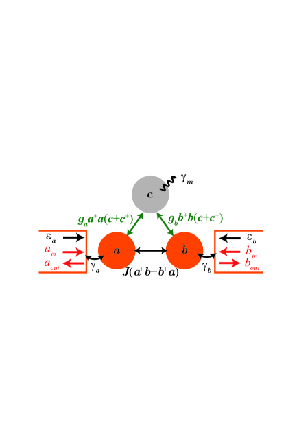
Figure 1: (Color online) Schematic diagram of an optomechanical system consisting of two optical modes ($a$ and $b$) and one mechanical mode ($c$). The optical modes and the mechanical mode are coupled via radiation pressure, respectively; meanwhile, the two optical modes are linearly coupled to each other.

We consider a three-mode optomechanical system LudwigPRL12 consisting of two optical modes ($a$ and $b$, frequencies $\omega_{a}$ and $\omega_{b}$) and one mechanical mode ($c$, frequency $\omega_{m}$) as shown in Fig. 1. The optomechanical coupling rates between the optical modes and the mechanical mode are denoted by $g_{a}$ and $g_{b}$; two optical modes are linearly coupled mutually at rate $J$ and driven by external laser sources with frequencies $\omega_{a,d}=\omega_{b,d}=\omega_{d}$ at rates $\varepsilon_{a}$ and $\varepsilon_{b}$ respectively. The Hamiltonian of the system in the rotating frame at the frequency of the driving fields $\omega_{d}$ is

$$H = \hbar\Delta_{a}a^{{\dagger}}a+\hbar\Delta_{b}b^{{\dagger}}b+\hbar\omega_{m}c^{{\dagger}}c+\hbar J\left(a^{{\dagger}}b+ab^{{\dagger}}\right)$$ (1)

$$+\hbar g_{a}a^{{\dagger}}a\left(c+c^{{\dagger}}\right)+\hbar g_{b}b^{{\dagger}}b\left(c+c^{{\dagger}}\right)$$

$$+i\hbar\left(\varepsilon_{a}a^{{\dagger}}e^{i\phi_{a}}+\varepsilon_{b}b^{{\dagger}}e^{i\phi_{b}}-\mathrm{H.c.}\right),$$

where $\Delta_{a}=\omega_{a}-\omega_{d}$ and $\Delta_{b}=\omega_{b}-\omega_{d}$ are the detunings between the optical modes and the driving fields. Without loss of generality, we assume that $J$, $\varepsilon_{a}$ and $\varepsilon_{b}$ are real and $\phi_{a}$ ($\phi_{b}$) is the phase of laser field coupling to the optical mode $a$ ($b$). This kind of Hamiltonian can be realized in the optomechanical system with a membrane in a Fabry-Pérot cavity ThompsonNat08 , microtoroid optomechanical cavities LinPRL09 , optomechanical crystals EichenfieldNat09 and electromechanical devices TeufelNat11 .

Substituting the Hamiltonian (1) into the Heisenberg equation and taking into account the damping and corresponding noise terms, we get the quantum Langevin equations (QLEs) for the operators of the optical and mechanical modes

$$\frac{d}{dt}a = \left\{-\frac{\gamma_{a}}{2}-i\left[\Delta_{a}+g_{a}\left(c+c^{{\dagger}}\right)\right]\right\}a-iJb$$ (2)

$$+\varepsilon_{a}e^{i\phi_{a}}+\sqrt{\gamma_{a}}a_{\mathrm{in}},$$

$$\frac{d}{dt}b = \left\{-\frac{\gamma_{b}}{2}-i\left[\Delta_{b}+g_{b}\left(c+c^{{\dagger}}\right)\right]\right\}b-iJa$$ (3)

$$+\varepsilon_{b}e^{i\phi_{b}}+\sqrt{\gamma_{b}}b_{\mathrm{in}},$$

$$\frac{d}{dt}c=\left(-\frac{\gamma_{m}}{2}-i\omega_{m}\right)c-i\left(g_{a}a^{{\dagger}}a+g_{b}b^{{\dagger}}b\right)+\sqrt{\gamma_{m}}c_{\mathrm{in}}.$$ (4)

Here, $\gamma_{a}$ ($\gamma_{b}$) is the damping rate of the optical mode $a$ ($b$) and $\gamma_{m}$ is the mechanical damping rate. $a_{\mathrm{in}}$, $b_{\mathrm{in}}$ and $c_{\mathrm{in}}$ are the input quantum fields with zero mean values, and the spectra of the input quantum fields, $s_{v,\mathrm{in}}\left(\omega\right)$, are defined via $\left\langle\widetilde{v_{\mathrm{in}}^{{\dagger}}}\left(\omega^{\prime}\right)\widetilde{v_{\mathrm{in}}}\left(\omega\right)\right\rangle=s_{v,\mathrm{in}}\left(\omega\right)\delta\left(\omega+\omega^{\prime}\right)$ and $\left\langle\widetilde{v_{\mathrm{in}}}\left(\omega^{\prime}\right)\widetilde{v_{\mathrm{in}}^{{\dagger}}}\left(\omega\right)\right\rangle=\left[1+s_{v,\mathrm{in}}\left(\omega\right)\right]\delta\left(\omega+\omega^{\prime}\right)$, where the term “1” results from the effect of vacuum noise and $\widetilde{v_{\mathrm{in}}^{{\dagger}}}$ ($\widetilde{v_{\mathrm{in}}}$) is the Fourier transform of $v_{\mathrm{in}}^{{\dagger}}$ ($v_{\mathrm{in}}$) for $v=a,b,c$.

The mean values of the operators in the steady state can be obtained from the nonlinear QLEs (2)-(4) by using factorization assumption like $\left\langle ca\right\rangle=\left\langle c\right\rangle\left\langle a\right\rangle$, and then

$$\left\langle a\right\rangle = \alpha=\frac{\left(\frac{\gamma_{b}}{2}+i\Delta_{b}^{\prime}\right)\varepsilon_{a}e^{i\phi_{a}}-iJ\varepsilon_{b}e^{i\phi_{b}}}{\left(\frac{\gamma_{a}}{2}+i\Delta_{a}^{\prime}\right)\left(\frac{\gamma_{b}}{2}+i\Delta_{b}^{\prime}\right)+J^{2}},$$ (5)

$$\left\langle b\right\rangle = \beta=\frac{\left(\frac{\gamma_{a}}{2}+i\Delta_{a}^{\prime}\right)\varepsilon_{b}e^{i\phi_{b}}-iJ\varepsilon_{a}e^{i\phi_{a}}}{\left(\frac{\gamma_{a}}{2}+i\Delta_{a}^{\prime}\right)\left(\frac{\gamma_{b}}{2}+i\Delta_{b}^{\prime}\right)+J^{2}},$$ (6)

$$\left\langle c\right\rangle = \xi=\frac{-i\left(g_{a}\left|\alpha\right|^{2}+g_{b}\left|\beta\right|^{2}\right)}{\left(\frac{\gamma_{m}}{2}+i\omega_{m}\right)},$$ (7)

where $\Delta_{a}^{\prime}=\Delta_{a}+g_{a}\left(\xi+\xi^{\ast}\right)$ and $\Delta_{b}^{\prime}=\Delta_{b}+g_{b}\left(\xi+\xi^{\ast}\right)$ are the effective detuning including the frequency shifts caused by the optomechanical interaction.

To solve the nonlinear QLEs (2)-(4), we linearize the equations in the strong driving condition (i.e., $\varepsilon_{a}\gg\gamma_{a}$, $\varepsilon_{b}\gg\gamma_{b}$), then the operators are rewritten as the sum of the mean values and the small quantum fluctuation terms i.e., $a=\alpha+\delta a$, $b=\beta+\delta b$, $c=\xi+\delta c$, where $\delta a\ll|\alpha|$ and $\delta b\ll|\beta|$. Substituting them into the nonlinear QLEs (2)-(4) and keeping only the first-order terms in the small quantum fluctuation terms $\delta a$, $\delta b$, and $\delta c$, we obtain the linearized QLEs

$$\frac{d}{dt}\delta a = \left(-\frac{\gamma_{a}}{2}-i\Delta_{a}^{\prime}\right)\delta a-iG_{a}\left(\delta c+\delta c^{{\dagger}}\right)$$ (8)

$$-iJ\delta b+\sqrt{\gamma_{a}}a_{\mathrm{in}},$$

$$\frac{d}{dt}\delta b = \left(-\frac{\gamma_{b}}{2}-i\Delta_{b}^{\prime}\right)\delta b-iG_{b}\left(\delta c+\delta c^{{\dagger}}\right)$$ (9)

$$-iJ\delta a+\sqrt{\gamma_{b}}b_{\mathrm{in}},$$

$$\frac{d}{dt}\delta c = \left(-\frac{\gamma_{m}}{2}-i\omega_{m}\right)\delta c-i\left(G_{a}\delta a^{{\dagger}}+G_{a}^{\ast}\delta a\right)$$ (10)

$$-i\left(G_{b}\delta b^{{\dagger}}+G_{b}^{\ast}\delta b\right)+\sqrt{\gamma_{m}}c_{\mathrm{in}},$$

where $G_{a}=g_{a}\alpha=|G_{a}|e^{i\theta_{a}}$ and $G_{b}=g_{b}\beta=|G_{b}|e^{i\theta_{b}}$ are the effective optomechanical coupling rates with phase difference $\theta\equiv\theta_{b}-\theta_{a}$.

For convenience, the linearized QLEs (8)-(10) can be concisely expressed as

$$\frac{d}{dt}V=-MV+\Gamma V_{\mathrm{in}},$$ (11)

where the fluctuation vector $V=\left(\delta a,\delta b,\delta c,\delta a^{{\dagger}},\delta b^{{\dagger}},\delta c^{{\dagger}}\right)^{T}$, the input field vector $V_{in}=\left(a_{\mathrm{in}},b_{\mathrm{in}},c_{\mathrm{in}},a_{\mathrm{in}}^{{\dagger}},b_{\mathrm{in}}^{{\dagger}},c_{\mathrm{in}}^{{\dagger}}\right)^{T}$, $\Gamma=\mathrm{diag}\left(\sqrt{\gamma_{a}},\sqrt{\gamma_{b}},\sqrt{\gamma_{m}},\sqrt{\gamma_{a}},\sqrt{\gamma_{b}},\sqrt{\gamma_{m}}\right)$ denotes the damping matrix and $M$ is the coefficient matrix

$$M=\left(\begin{array}[]{cccccc}\frac{\gamma_{a}}{2}+i\Delta_{a}^{\prime}&iJ&iG_{a}&0&0&iG_{a}\\ iJ&\frac{\gamma_{b}}{2}+i\Delta_{b}^{\prime}&iG_{b}&0&0&iG_{b}\\ iG_{a}^{\ast}&iG_{b}^{\ast}&\frac{\gamma_{m}}{2}+i\omega_{m}&iG_{a}&iG_{b}&0\\ 0&0&-iG_{a}^{\ast}&\frac{\gamma_{a}}{2}-i\Delta_{a}^{\prime}&-iJ&-iG_{a}^{\ast}\\ 0&0&-iG_{b}^{\ast}&-iJ&\frac{\gamma_{b}}{2}-i\Delta_{b}^{\prime}&-iG_{b}^{\ast}\\ -iG_{a}^{\ast}&-iG_{b}^{\ast}&0&-iG_{a}&-iG_{b}&\frac{\gamma_{m}}{2}-i\omega_{m}\end{array}\right).$$ (12)

Due to the stability condition, the real parts of all the eigenvalues of matrix $M$ have to be positive. By introducing the Fourier transform of the operators

$$\widetilde{o}\left(\omega\right) = \frac{1}{\sqrt{2\pi}}\int_{-\infty}^{+\infty}o\left(t\right)e^{i\omega t}dt,$$ (13)

$$\widetilde{o^{{\dagger}}}\left(\omega\right) = \frac{1}{\sqrt{2\pi}}\int_{-\infty}^{+\infty}o^{{\dagger}}\left(t\right)e^{i\omega t}dt,$$ (14)

(for any operator $o$) and using the properties of Fourier transformation, the solution to the linearized QLEs (11) in the frequency domain is

$$\widetilde{V}\left(\omega\right)=\left(M-i\omega I\right)^{-1}\Gamma\widetilde{V}_{\mathrm{in}}\left(\omega\right),$$ (15)

where $I$ denotes the identity matrix.

As a consequence of boundary conditions, the relation among the input, internal, and output fields is given as the fol1owing GardinerPRA85

$$v_{\mathrm{out}}+v_{\mathrm{in}}=\sqrt{\gamma_{v}}\delta v$$ (16)

for $v=a,b,c$, and $\gamma_{c}\equiv\gamma_{m}$. Then the output field vector in the frequency domain is

$$\widetilde{V}_{\mathrm{out}}\left(\omega\right)=U\left(\omega\right)\widetilde{V}_{\mathrm{in}}\left(\omega\right),$$ (17)

where the output field vector $\widetilde{V}_{\mathrm{out}}\left(\omega\right)$ is the Fourier transform of $V_{\mathrm{out}}=\left(a_{\mathrm{out}},b_{\mathrm{out}},c_{\mathrm{out}},a_{\mathrm{out}}^{{\dagger}},b_{\mathrm{out}}^{{\dagger}},c_{\mathrm{out}}^{{\dagger}}\right)^{T}$ and

$$U\left(\omega\right)=\Gamma\left(M-i\omega I\right)^{-1}\Gamma-I.$$ (18)

The spectrum of the output fields is defined by

$$s_{v,\mathrm{out}}\left(\omega\right)=\int d\omega^{\prime}\left\langle\widetilde{v_{\mathrm{out}}^{{\dagger}}}\left(\omega^{\prime}\right)\widetilde{v_{\mathrm{out}}}\left(\omega\right)\right\rangle.$$ (19)

By substituting the expression of $\widetilde{V}_{\mathrm{out}}\left(\omega\right)$ [Eq. (17)] into Eq. (19), one can obtain AgarwalPRA12

$$S_{\mathrm{out}}\left(\omega\right)=T\left(\omega\right)S_{\mathrm{in}}\left(\omega\right)+S_{\mathrm{vac}}\left(\omega\right).$$ (20)

Here $S_{\mathrm{in}}\left(\omega\right)=\left(s_{a,\mathrm{in}}\left(\omega\right),s_{b,\mathrm{in}}\left(\omega\right),s_{c,\mathrm{in}}\left(\omega\right)\right)^{T}$, $S_{\mathrm{out}}\left(\omega\right)=\left(s_{a,\mathrm{out}}\left(\omega\right),s_{b,\mathrm{out}}\left(\omega\right),s_{c,\mathrm{out}}\left(\omega\right)\right)^{T}$, $S_{\mathrm{vac}}\left(\omega\right)=\left(s_{a,\mathrm{vac}}\left(\omega\right),s_{b,\mathrm{vac}}\left(\omega\right),s_{c,\mathrm{vac}}\left(\omega\right)\right)^{T}$, and

$$T\left(\omega\right)=\left(\begin{array}[]{ccc}T_{aa}\left(\omega\right)&T_{ab}\left(\omega\right)&T_{ac}\left(\omega\right)\\ T_{ba}\left(\omega\right)&T_{bb}\left(\omega\right)&T_{bc}\left(\omega\right)\\ T_{ca}\left(\omega\right)&T_{cb}\left(\omega\right)&T_{cc}\left(\omega\right)\end{array}\right),$$ (21)

where the element $T_{ij}\left(\omega\right)$ ($i,j=a,b,c$) denotes the scattering probability that is corresponding to the output field of $i$ mode arising from the presence of a single photon (or single phonon) in the input field of $j$ mode. The scattering probabilities are given as

$$T_{aa}\left(\omega\right) = \left|U_{11}\left(\omega\right)\right|^{2}+\left|U_{14}\left(\omega\right)\right|^{2},$$ (22)

$$T_{ab}\left(\omega\right) = \left|U_{12}\left(\omega\right)\right|^{2}+\left|U_{15}\left(\omega\right)\right|^{2},$$ (23)

$$T_{ac}\left(\omega\right) = \left|U_{13}\left(\omega\right)\right|^{2}+\left|U_{16}\left(\omega\right)\right|^{2},$$ (24)

$$T_{ba}\left(\omega\right) = \left|U_{21}\left(\omega\right)\right|^{2}+\left|U_{24}\left(\omega\right)\right|^{2},$$ (25)

$$T_{bb}\left(\omega\right) = \left|U_{22}\left(\omega\right)\right|^{2}+\left|U_{25}\left(\omega\right)\right|^{2},$$ (26)

$$T_{bc}\left(\omega\right) = \left|U_{23}\left(\omega\right)\right|^{2}+\left|U_{26}\left(\omega\right)\right|^{2},$$ (27)

$$T_{ca}\left(\omega\right) = \left|U_{31}\left(\omega\right)\right|^{2}+\left|U_{34}\left(\omega\right)\right|^{2},$$ (28)

$$T_{cb}\left(\omega\right) = \left|U_{32}\left(\omega\right)\right|^{2}+\left|U_{35}\left(\omega\right)\right|^{2},$$ (29)

$$T_{cc}\left(\omega\right) = \left|U_{33}\left(\omega\right)\right|^{2}+\left|U_{36}\left(\omega\right)\right|^{2},$$ (30)

where $U_{ij}\left(\omega\right)$ (for $i,j=1,\cdots,6$) represents the element at the $i$th row and $j$th column of the matrix $U\left(\omega\right)$ given by Eq. (18). $s_{v,\mathrm{vac}}$ ($v=a,b,c$) is the output spectrum contributing from the input vacuum field,

$$s_{a,\mathrm{vac}}\left(\omega\right) = \left|U_{14}\left(\omega\right)\right|^{2}+\left|U_{15}\left(\omega\right)\right|^{2}+\left|U_{16}\left(\omega\right)\right|^{2},$$ (31)

$$s_{b,\mathrm{vac}}\left(\omega\right) = \left|U_{24}\left(\omega\right)\right|^{2}+\left|U_{25}\left(\omega\right)\right|^{2}+\left|U_{26}\left(\omega\right)\right|^{2},$$ (32)

$$s_{c,\mathrm{vac}}\left(\omega\right) = \left|U_{34}\left(\omega\right)\right|^{2}+\left|U_{35}\left(\omega\right)\right|^{2}+\left|U_{36}\left(\omega\right)\right|^{2}.$$ (33)

III Optical nonreciprocity

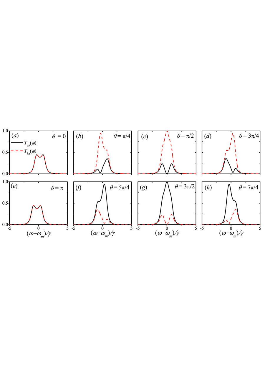
Figure 2: (Color online) Scattering probabilities $T_{ab}\left(\omega\right)$ (black solid lines) and $T_{ba}\left(\omega\right)$ (red dash lines) as functions of the frequency of the incoming signal $\omega$ for different phase difference: (a) $\theta=0$; (b) $\theta=\pi/4$; (c) $\theta=\pi/2$; (d) $\theta=3\pi/4$; (e) $\theta=\pi$; (f) $\theta=5\pi/4$; (g) $\theta=3\pi/2$; (h) $\theta=7\pi/4$. The other parameters are $\Delta_{a}^{\prime}=\Delta_{b}^{\prime}=\omega_{m}=10\gamma$, $J=G_{a}=G_{b}e^{-i\theta}=\gamma_{a}/2=\gamma_{b}/2=\gamma_{m}/2=\gamma/2$.

In this and next sections, we numerically evaluate the scattering probabilities to show the possibility of optical nonreciprocal response and optomechanical circulator behavior in the three-mode optomechanical system. The optimal parameters for the observation of optical nonreciprocal response are obtained according to the numerical results. The physical origin for the optical nonreciprocal response and optomechanical circulator behavior will be discussed in the next section.

Scattering probabilities $T_{ab}\left(\omega\right)$ and $T_{ba}\left(\omega\right)$ as functions of the frequency of the incoming signal $\omega$ for different phase difference are shown in Fig. 2, where the parameters are $\Delta_{a}^{\prime}=\Delta_{b}^{\prime}=\omega_{m}=10\gamma$, $J=G_{a}=G_{b}e^{-i\theta}=\gamma_{a}/2=\gamma_{b}/2=\gamma_{m}/2=\gamma/2$. The photon transmission satisfies the Lorentz reciprocal theorem [e.g. $T_{ab}\left(\omega\right)=T_{ba}\left(\omega\right)$] on the condition that $\theta=0$ or $\pi$. In the regime $0<\theta<\pi$, we have $T_{ab}\left(\omega\right)<T_{ba}\left(\omega\right)$; in the regime $\pi<\theta<2\pi$, we have $T_{ab}\left(\omega\right)>T_{ba}\left(\omega\right)$. The optimal optical nonreciprocal response is obtained as $\theta=\pi/2$ [$T_{ab}\left(\omega\right)\approx 0$ and $T_{ba}\left(\omega\right)\approx 1$ at $\omega=\omega_{m}$] and $\theta=3\pi/2$ [$T_{ab}\left(\omega\right)\approx 1$ and $T_{ba}\left(\omega\right)\approx 0$ at $\omega=\omega_{m}$]. The condition of $G_{a}=G_{b}e^{-i\theta}=\gamma/2$ with $g_{a}=g_{b}=g$ can be obtained approximately by setting the amplitudes and the phases of the coupling laser fields as

$$\varepsilon_{a}=\varepsilon_{b}\approx\frac{\gamma\omega_{m}}{2g},$$ (34)

$$\phi_{a}=\phi_{b}-\theta\approx\frac{\pi}{2}.$$ (35)

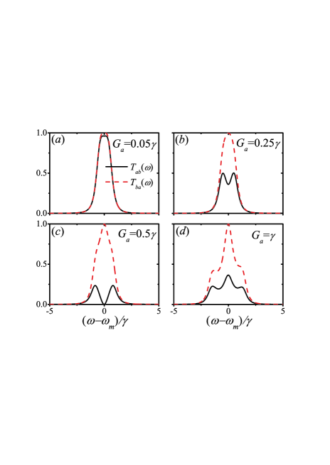
Figure 3: (Color online) Scattering probabilities $T_{ab}\left(\omega\right)$ (black solid line) and $T_{ba}\left(\omega\right)$ (red dash line) as functions of the frequency of the incoming signal $\omega$ for different effective optomechanical coupling rates: (a) $G_{a}=0.05\gamma$; (b) $G_{a}=0.25\gamma$; (c) $G_{a}=0.5\gamma$; (d) $G_{a}=\gamma$. The other parameters are $\Delta_{a}^{\prime}=\Delta_{b}^{\prime}=\omega_{m}=10\gamma$, $J=\gamma_{a}/2=\gamma_{b}/2=\gamma_{m}/2=\gamma/2$. Here we fix $G_{b}=iG_{a}$ which corresponds to the case of $\theta=\pi/2$.

In Fig. 3, the scattering probabilities $T_{ab}\left(\omega\right)$ and $T_{ba}\left(\omega\right)$ are shown as functions of the frequency of the incoming signal $\omega$ for different effective optomechanical coupling rates $G_{a}$ with the parameters: $\Delta_{a}^{\prime}=\Delta_{b}^{\prime}=\omega_{m}=10\gamma$, $J=\gamma_{a}/2=\gamma_{b}/2=\gamma_{m}/2=\gamma/2$, $G_{b}=iG_{a}$. It is shown that as the effective optomechanical coupling is weak ($\{|G_{a}|,|G_{b}|\}\ll\gamma$), the scattering probability from $b$ mode to $a$ mode is almost the same as the one from $a$ mode to $b$ mode, e.g., $T_{ab}\left(\omega\right)\approx T_{ba}\left(\omega\right)$. With the enhancement of the effective optomechanical coupling rates, the optical nonreciprocal response becomes obvious and gets to the optimal effect at about $G_{a}=0.5\gamma$.

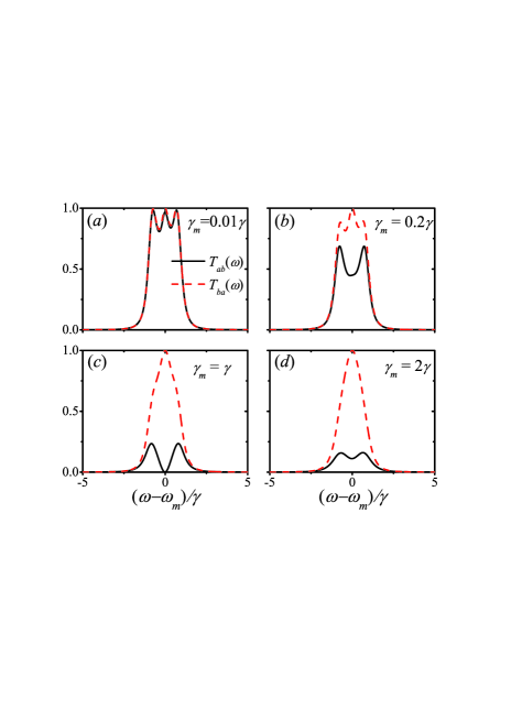
Figure 4: (Color online) Scattering probabilities $T_{ab}\left(\omega\right)$ (black solid lines) and $T_{ba}\left(\omega\right)$ (red dash lines) as functions of the frequency of the incoming signal $\omega$ for different mechanical damping rates: (a) $\gamma_{m}=0.01\gamma$; (b) $\gamma_{m}=0.2\gamma$; (c) $\gamma_{m}=\gamma$; (d) $\gamma_{m}=2\gamma$. The other parameters are $\Delta_{a}^{\prime}=\Delta_{b}^{\prime}=\omega_{m}=10\gamma$, $J=G_{a}=-iG_{b}=\gamma_{a}/2=\gamma_{b}/2=\gamma/2$.

In Fig. 4, we plot the scattering probabilities $T_{ab}\left(\omega\right)$ and $T_{ba}\left(\omega\right)$ for different mechanical damping rates $\gamma_{m}$ with the parameters: $\Delta_{a}^{\prime}=\Delta_{b}^{\prime}=\omega_{m}=10\gamma$, $J=G_{a}=-iG_{b}=\gamma_{a}/2=\gamma_{b}/2=\gamma/2$. It is shown that as the mechanical damping rates $\gamma_{m}$ is much smaller than the optical damping rate ($\gamma_{m}\ll\gamma$), the photon scattering probabilities are almost the same for the two directions, e.g. $T_{ab}\left(\omega\right)\approx T_{ba}\left(\omega\right)$. With the increase of the mechanical damping rate, the optical nonreciprocal response becomes obvious and achieves the optimal effect for $\gamma_{m}\approx\gamma$.

IV Optomechanical circulator

As done in most of the studies on optomechanical systems, the signal input and/or output from the mechanical mode is not considered in last section. With the development of phonon-based system, phonon is another useful media for quantum information processing HabrakenNJP12 . In this section, we assume that the mechanical mode is coupled to a continuous mode of phonon waveguide and the phonons can be input and output through the phonon waveguide. The scattering of both photons and phonons in the three-mode optomechanical system is considered in the following.

Using Eqs. (22)-(30), we now show the numerical results of all the scattering probabilities (nine elements) in Eqs. (21). As shown in Fig. 5, the three-mode optomechanical system shows circulator behavior: when $\theta=\pi/2$, we have $T_{ba}\left(\omega\right)\approx T_{cb}\left(\omega\right)\approx T_{ac}\left(\omega\right)\approx 1$ and the other scattering probabilities equal to zero at $\omega=\omega_{m}$ as shown in Figs. 5 (a), (c) and (e); when $\theta=3\pi/2$, we have $T_{ca}\left(\omega\right)\approx T_{ab}\left(\omega\right)\approx T_{bc}\left(\omega\right)\approx 1$ and the other scattering probabilities equal to zero at $\omega=\omega_{m}$ as shown in Figs. 5 (b), (d) and (f). That is to say the signal is transferred from one mode to another either counterclockwisely ($a\rightarrow b\rightarrow c\rightarrow a$) or clockwisely ($a\rightarrow c\rightarrow b\rightarrow a$), depending on the relative phase $\theta=\pi/2$ or $3\pi/2$ as shown in Fig. 6.

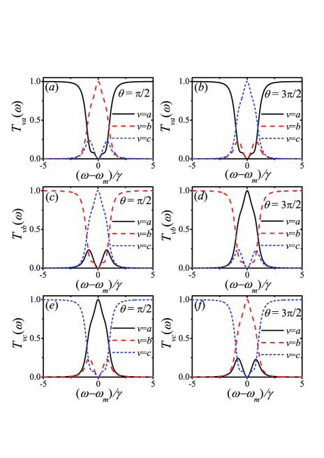
Figure 5: (Color online) Scattering probabilities $T_{va}\left(\omega\right)$ [(a) and (b)], $T_{vb}\left(\omega\right)$ [(c) and (d)] and $T_{vc}\left(\omega\right)$ [(e) and (f)] ($v=a,b,c$) as functions of the frequency of the incoming signal $\omega$ for different phase difference: (a), (c) and (e) $\theta=\pi/2$; (b), (d) and (f) $\theta=3\pi/2$. The other parameters are $\Delta_{a}^{\prime}=\Delta_{b}^{\prime}=\omega_{m}=10\gamma$, $J=G_{a}=G_{b}e^{-i\theta}=\gamma_{a}/2=\gamma_{b}/2=\gamma_{m}/2=\gamma/2$.

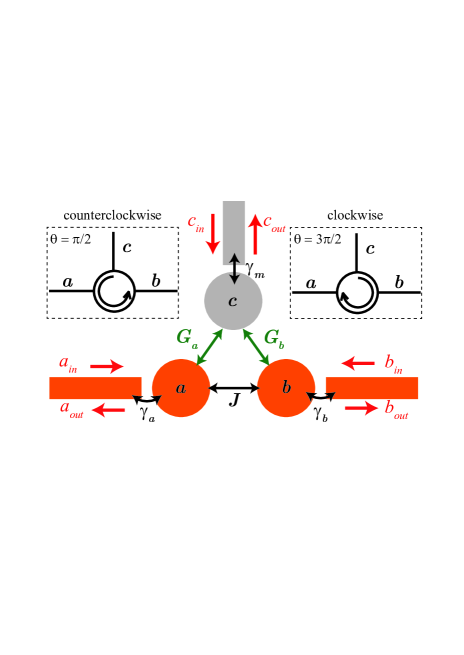
Figure 6: (Color online) Schematic diagram of a three-mode optomechanical circulator.

The scattering matrix for the optomechanical circulator in three-mode optomechanical systems can be obtained analytically, similar to the case for photon and phonon circulators in Refs. KochPRA10 ; HabrakenNJP12 . We assume that $\omega_{m}\approx\Delta\gg\{J,\left|G_{a}\right|,\left|G_{b}\right|,\gamma_{a},\gamma_{b},\gamma_{m}$}, then Eqs. (8)-(10) can be simplified by rotating wave approximation as

$$\frac{d}{dt}\delta a=\left(-\frac{\gamma_{a}}{2}-i\Delta_{a}^{\prime}\right)\delta a-iG_{a}\delta c-iJ\delta b+\sqrt{\gamma_{a}}a_{\mathrm{in}},$$ (36)

$$\frac{d}{dt}\delta b=\left(-\frac{\gamma_{b}}{2}-i\Delta_{b}^{\prime}\right)\delta b-iG_{b}\delta c-iJ\delta a+\sqrt{\gamma_{b}}b_{\mathrm{in}},$$ (37)

$$\frac{d}{dt}\delta c=\left(-\frac{\gamma_{m}}{2}-i\omega_{m}\right)\delta c-iG_{a}^{\ast}\delta a-iG_{b}^{\ast}\delta b+\sqrt{\gamma_{m}}c_{\mathrm{in}}.$$ (38)

Thus the effective Hamiltonian after linearization takes the form (effective system is shown in Fig. 6)

$$H_{\mathrm{eff}} = \hbar\Delta_{a}^{\prime}a^{{\dagger}}a+\hbar\Delta_{b}^{\prime}b^{{\dagger}}b+\hbar\omega_{m}c^{{\dagger}}c$$

$$+\hbar\left(Jb^{{\dagger}}a+|G_{a}|e^{i\theta_{a}}a^{{\dagger}}c+|G_{b}|e^{-i\theta_{b}}c^{{\dagger}}b+\mathrm{H.c.}\right).$$

The necessary and sufficient condition of time-reversal symmetry is the gauge-invariant phase sum is an integral multiple of $\pi$ KochPRA10 . That is,

$$\theta_{b}-\theta_{a}\equiv\theta=n\pi$$ (40)

for real $J$, where $n$ is an integral number [also see the numerical results as shown in Figs. 2(a) and 2(e)]. The optical nonreciprocal response and the optomechanical circulator behavior are induced by breaking the time-reversal symmetry (i.e., $\theta_{b}-\theta_{a}\neq n\pi$), and the optimal effect is realized at the halfway between the time-reversal symmetric points (i.e., $\theta_{a}=0$, $\theta_{b}=\theta=\pi/2$ or $3\pi/2$) as shown in Fig. 5.

Now we will derive the scattering matrix of the optomechanical circulator behavior analytically from the simplified linearized QLEs [Eqs. (36)-(38)]. Let us transform the linearized equations into the frequency domain,

$$\left(M^{\prime}-i\omega I\right)\left(\begin{array}[]{c}\widetilde{\delta a}\\ \widetilde{\delta b}\\ \widetilde{\delta c}\end{array}\right)=\left(\begin{array}[]{c}\sqrt{\gamma_{a}}\widetilde{a_{\mathrm{in}}}\\ \sqrt{\gamma_{b}}\widetilde{b_{\mathrm{in}}}\\ \sqrt{\gamma_{m}}\widetilde{c_{\mathrm{in}}}\end{array}\right),$$ (41)

where

$$M^{\prime}=\left(\begin{array}[]{ccc}\frac{\gamma_{a}}{2}+i\Delta_{a}^{\prime}&iJ&iG_{a}\\ iJ&\frac{\gamma_{b}}{2}+i\Delta_{b}^{\prime}&iG_{b}\\ iG_{a}^{\ast}&iG_{b}^{\ast}&\frac{\gamma_{m}}{2}+i\omega_{m}\end{array}\right).$$ (42)

In the conditions for the optimal optomechanical circulator, i.e. $\omega=\Delta_{a}^{\prime}=\Delta_{b}^{\prime}=\omega_{m}$ and $J=G_{a}=G_{b}e^{-i\theta}=\gamma_{a}/2=\gamma_{b}/2=\gamma_{m}/2=\gamma/2$, we have

$$\frac{\gamma}{2}\left(\begin{array}[]{ccc}1&i&i\\ i&1&ie^{i\theta}\\ i&ie^{-i\theta}&1\end{array}\right)\left(\begin{array}[]{c}\widetilde{\delta a}\\ \widetilde{\delta b}\\ \widetilde{\delta c}\end{array}\right)=\left(\begin{array}[]{c}\sqrt{\gamma}\widetilde{a_{\mathrm{in}}}\\ \sqrt{\gamma}\widetilde{b_{\mathrm{in}}}\\ \sqrt{\gamma}\widetilde{c_{\mathrm{in}}}\end{array}\right).$$ (43)

By choosing $\theta=\pi/2$, the scattering matrix is given through

$$\left(\begin{array}[]{c}\widetilde{a_{\mathrm{out}}}\\ \widetilde{b_{\mathrm{out}}}\\ \widetilde{c_{\mathrm{out}}}\end{array}\right)=\left(\begin{array}[]{ccc}0&0&-i\\ -i&0&0\\ 0&-1&0\end{array}\right)\left(\begin{array}[]{c}\widetilde{a_{\mathrm{in}}}\\ \widetilde{b_{\mathrm{in}}}\\ \widetilde{c_{\mathrm{in}}}\end{array}\right).$$ (44)

By choosing $\theta=3\pi/2$, we can get the scattering matrix through

$$\left(\begin{array}[]{c}\widetilde{a_{\mathrm{out}}}\\ \widetilde{b_{\mathrm{out}}}\\ \widetilde{c_{\mathrm{out}}}\end{array}\right)=\left(\begin{array}[]{ccc}0&-i&0\\ 0&0&-1\\ -i&0&0\end{array}\right)\left(\begin{array}[]{c}\widetilde{a_{\mathrm{in}}}\\ \widetilde{b_{\mathrm{in}}}\\ \widetilde{c_{\mathrm{in}}}\end{array}\right).$$ (45)

Equation (44) shows clearly a perfect circulator with the signal transferring counterclockwisely ($a\rightarrow b\rightarrow c\rightarrow a$) for $\theta=\pi/2$ and Eq. (45) also describes an ideal circulator but with the signal transferring clockwisely ($a\rightarrow c\rightarrow b\rightarrow a$) for $\theta=3\pi/2$. These agree well with the numerical results shown in Fig. 5.

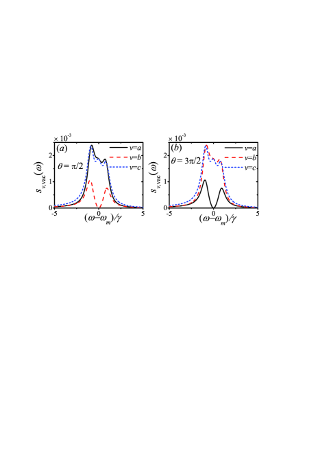
Figure 7: (Color online) The vacuum noise spectrum $s_{v,\mathrm{vac}}\left(\omega\right)$ ($v=a,b,c$) as a function of the frequency of the incoming signal $\omega$ for different phase difference: (a) $\theta=\pi/2$; (b) $\theta=3\pi/2$. The other parameters are $\Delta_{a}^{\prime}=\Delta_{b}^{\prime}=\omega_{m}=10\gamma$, $J=G_{a}=G_{b}e^{-i\theta}=\gamma_{a}/2=\gamma_{b}/2=\gamma_{m}/2=\gamma/2$.

Finally, we discuss the effects of the vacuum noise spectrum $s_{v,\mathrm{vac}}\left(\omega\right)$ given by Eqs. (31)-(33). The vacuum noise spectrum $s_{v,\mathrm{vac}}\left(\omega\right)$ ($v=a,b,c$) as a function of the frequency of the incoming signal $\omega$ is shown in Fig. 7. The effects of the vacuum noises are so small that they are insignificant even for the input signals of single-photon (single-phonon) level (about $0.2\%$ at $\omega=\omega_{m}=10\gamma$). The physical origin of the vacuum noise in the output spectrum is the anti-rotating-wave interactions between the optical and the mechanical modes [included in Eq. (11)]. The suppression of the vacuum noise for $b$ mode ($a$ mode) at $\omega=\omega_{m}$ as $\theta=\pi/2$ ($\theta=3\pi/2$) is the consequence of the rotating-wave approximation for the interaction between the two optical modes.

V Conclusions

In summary, we have shown the optical nonreciprocity in a three-mode optomechanical system. We demonstrated that the nonreciprocal response is enabled by tuning the phase difference between the optomechanical coupling rates to induce the time-reversal symmetry breaking of the system. Then we show that the three-mode optomechanical system can also be used as a three-port optomechanical circulator for two optical modes and one mechanical mode. Further, we note that the three-mode optomechanical system can work in the single-photon level and be integrated into a chip. The three-port optomechanical circulator might eventually provide the basis for applications on quantum information processing or quantum simulation NunnenkampNJP11 .

Note added

In the preparation of this work, we became aware of a related paper by Metelmann and Clerk Metelmann15arx .

Acknowledgement

We thank W. H. Hu for fruitful discussions. This work is supported by the Postdoctoral Science Foundation of China (under Grant No. 2014M550019), the National Natural Science Foundation of China (under Grants No. 11422437, No. 11174027, and No. 11121403) and the National Basic Research Program of China (under Grants No. 2012CB922104 and No. 2014CB921403).

References

• (1) R. J. Potton, Rep. Prog. Phys. 67, 717 (2004); I.V. Shadrivov, V. A. Fedotov, D. A. Powell, Y. S. Kivshar, and N. I. Zheludev, New J. Phys. 13, 033025 (2011).
• (2) J. Fujita, M. Levy, R. M. Osgood, L.Wilkens, and H. Dötsch, Appl. Phys. Lett. 76, 2158 (2000); R. L. Espinola, T. Izuhara, M. C. Tsai, R. M. Osgood Jr., H. Dötsch, Opt. Lett. 29, 941 (2004); T. R. Zaman, X. Guo, R. J. Ram, Appl. Phys. Lett. 90, 023514 (2007); F. D. M. Haldane and S. Raghu, Phys. Rev. Lett. 100, 013904 (2008); Y. Shoji, T. Mizumoto, H. Yokoi, I. Hsieh, and R. M. Osgood, Appl. Phys. Lett. 92, 071117 (2008); Z. Wang, Y. Chong, J. D. Joannopoulos, and M. Soljačić, Nature (London) 461, 772 (2009); Y. Hadad and B. Z. Steinberg, Phys. Rev. Lett. 105, 233904 (2010); A. B. Khanikaev, S. H. Mousavi, G. Shvets, and Y. S. Kivshar, ibid. 105, 126804 (2010); L. Bi, J. Hu, P. Jiang, D. H. Kim, G. F. Dionne, L. C. Kimerling, and C. A. Ross, Nat. Photon. 5, 758 (2011); Y. Shoji, M. Ito, Y. Shirato, and T. Mizumoto, Opt. Express 20, 18440 (2012).
• (3) K. Gallo, G. Assanto, K. R. Parameswaran, and M. M. Fejer, Appl. Phys. Lett. 79, 314 (2001); S. F. Mingaleev, Y. S. Kivshar, J. Opt. Soc. Am. B 19, 2241 (2002); M. Soljačić, C. Luo, J. D. Joannopoulos, S. Fan, Opt. Lett. 28, 637 (2003); A. Rostami, Opt. Laser Technol. 39, 1059 (2007); A. Alberucci and G. Assanto, Opt. Lett. 33, 1641 (2008); L. Fan, J. Wang, L. T. Varghese, H. Shen, B. Niu, Y. Xuan, A. M. Weiner, and M. Qi, Science 335, 447 (2012); L. Fan, L. T. Varghese, J. Wang, Y. Xuan, A. M. Weiner, and M. Qi, Opt. Lett. 38, 1259 (2013); B. Anand, R. Podila, K. Lingam, S. R. Krishnan, S. S. S. Sai, R. Philip, and A. M. Rao, Nano Lett. 13, 5771 (2013).
• (4) F. Biancalana, J. Appl. Phys. 104, 093113(2008); A. E. Miroshnichenko, E. Brasselet, and Y. S. Kivshar, Appl. Phys. Lett. 96, 063302 (2010); C. Wang, C. Zhou, and Z. Li, Opt. Express 19, 26948 (2011); C. Wang, X. Zhong, and Z. Li, Sci. Rep. 2, 674 (2012); K. Xia, M. Alamri, and M. S. Zubairy, Opt. Express 21, 25619 (2013); E. J. Lenferink, G. Wei, and N. P. Stern, ibid. 22, 16099 (2014); Y. Yu, Y. Chen, H. Hu, W. Xue, K. Yvind, and J. Mork, arXiv:1409.3147.
• (5) Z. F. Yu and S. H. Fan, Nat. Photon. 3, 91 (2009); K. Fang, Z. Yu, and S. Fan, ibid. 6, 782 (2012); E. Li, B. J. Eggleton, K. Fang, and S. Fan, Nat. Commun. 5, 3225 (2014); C. R. Doerr, N. Dupuis, and L. Zhang, Opt. Lett. 36, 4293 (2011); C. R. Doerr, L. Chen, and D. Vermeulen, Opt. Express 22, 4493 (2014); H. Lira, Z. F. Yu, S. H. Fan, and M. Lipson, Phys. Rev. Lett. 109, 033901 (2012); K. Fang, Z. Yu, and S. Fan, ibid. 108, 153901 (2012); M. C. Munoz, A. Y. Petrov, L. O’Faolain, J. Li, T. F. Krauss, and M. Eich, ibid. 112, 053904 (2014); Y. Yang, C. Galland, Y. Liu, K. Tan, R. Ding, Q. Li, K. Bergman, T. Baehr-Jones, and M. Hochberg, Opt. Express 22, 17409 (2014).
• (6) Q. Wang, F. Xu, Z. Y. Yu, X. S. Qian, X. K. Hu, Y. Q. Lu, and H. T. Wang, Opt. Express 18, 7340 (2010); M. S. Kang, A. Butsch, and P. S. J. Russell, Nat. Photon. 5, 549 (2011).
• (7) C. Eüter, K. G. Makris, R. EI-Ganainy, D. N. Christodoulides, M. Segev, and D. Kip, Nat. Phys. 6, 192 (2010); H. Ramezani, T. Kottos, R. El-Ganainy, and D. N. Christodoulides, Phys. Rev. A 82, 043803 (2010); L. Feng, M. Ayache, J. Q. Huang, Y. L. Xu, M. H. Lu, Y. F. Chen, Y. Fainman, and A. Scherer, Science 333, 729 (2011); B. Peng, S. K. Özdemir, F. Lei, F. Monifi, M. Gianfreda, G. L. Long, S. H. Fan, F. Nori, C. M. Bender, and L. Yang, Nat. Phys. 10, 394 (2014); J. H. Wu, M. Artoni, and G. C. La Rocca, Phys. Rev. Lett. 113, 123004 (2014).
• (8) D. W. Wang, H. T. Zhou, M. J. Guo, J. X. Zhang, J. Evers, and S. Y. Zhu, Phys. Rev. Lett. 110, 093901 (2013); S. A. R. Horsley, J. H. Wu, M. Artoni, and G. C. La Rocca, ibid. 110, 223602 (2013).
• (9) Y. Shen, M. Bradford, and J. T. Shen, Phys. Rev. Lett. 107, 173902 (2011); K. Xia, G. Lu, G. Lin, Y. Cheng, Y. Niu, S. Gong, and J. Twamley, Phys. Rev. A 90, 043802 (2014); H. Z. Shen, Y. H. Zhou, and X. X. Yi, ibid. 90, 023849 (2014).
• (10) T. J. Kippenberg and K. J. Vahala, Science 321, 1172 (2008); F. Marquardt and S. M. Girvin, Physics 2, 40 (2009); M. Aspelmeyer, P. Meystre, and K. Schwab, Phys. Today 65, 29 (2012); M. Aspelmeyer, T. J. Kippenberg, and F. Marquardt, Rev. Mod. Phys. 86, 1391 (2014).
• (11) S. Manipatruni, J. T. Robinson, and M. Lipson, Phys. Rev. Lett. 102, 213903 (2009).
• (12) M. Hafezi and P. Rabl, Opt. Express 20, 7672 (2012).
• (13) J. Koch, A. A. Houck, K. L. Hur, and S. M. Girvin, Phys. Rev. A 82, 043811 (2010).
• (14) S. J. M. Habraken, K. Stannigel, M. D. Lukin, P. Zoller, and P Rabl, New J. Phys. 14, 115004 (2012).
• (15) M. Ludwig, A. H. Safavi-Naeini, O. Painter, and F. Marquardt, Phys. Rev. Lett. 109, 063601 (2012); K. Stannigel, P. Komar, S. J. M. Habraken, S. D. Bennett, M. D. Lukin, P. Zoller, and P. Rabl, ibid. 109, 013603 (2012); Y. D. Wang and A. A. Clerk, ibid. 108, 153603 (2012); L. Tian, ibid. 108, 153604 (2012); W. J. Gu and G. X. Li, Phys. Rev. A 87, 025804 (2013).
• (16) J. D. Thompson, B. M. Zwickl, A. M. Jayich, F. Marquardt, S. M. Girvin, and J. G. E. Harris, Nature (London) 452, 72 (2008); G. Heinrich, J. G. E. Harris, and F. Marquardt, Phys. Rev. A 81, 011801(R) (2010); H. Z. Wu, G. Heinrich, and F. Marquardt, New J. Phys. 15, 123022 (2013).
• (17) Q. Lin, J. Rosenberg, X. Jiang, K. J. Vahala, and O. Painter, Phys. Rev. Lett. 103, 103601 (2009); S. Weis, R. Rivière. S. Deléglise, E. Gavartin, O. Arcizet, A. Schliesser, and T. J. Kippenberg, Science 330, 1520 (2010).
• (18) M. Eichenfield, R. Camacho, J. Chan, K. J. Vahala, and O. Painter, Nature (London) 459, 550 (2009); M. Li, W. H. P. Pernice, and H. X. Tang, Nat. Photon. 3, 464 (2009); A. H. Safavi-Naeini and O. Painter, New J. Phys. 13, 013017 (2011); J. T. Hill, A. H. Safavi-Naeini, J. Chan, and O. Painter, Nat. Commun. 3, 1196 (2012).
• (19) J. D. Teufel, D. Li, M. S. Allman, K. Cicak, A. J. Sirois, J. D. Whittaker, and R. W. Simmonds, Nature (London) 471, 204 (2011); F. Massel, S. Un Cho, J.-M. Pirkkalainen, P. J. Hakonen, T. T. Heikkilä, and M. A. Sillanpää, Nat. Commun. 3, 987 (2012); T. A. Palomaki, J. D. Teufel, R. W. Simmonds, and K. W. Lehnert, Science 342, 710 (2013); J. Suh, A. J. Weinstein, C. U. Lei, E. E. Wollman, S. K. Steinke, P. Meystre, A. A. Clerk, and K. C. Schwab, ibid. 344, 1262 (2014).
• (20) C. W. Gardiner and M. J. Collett, Phys. Rev. A 31, 3761 (1985).
• (21) G. S. Agarwal and S. Huang, Phys. Rev. A 85, 021801(R) (2012).
• (22) A. Nunnenkamp, J. Koch, and S. M. Girvin, New J. Phys. 13, 095008 (2011); A. L. C. Hayward, A. M. Martin, and A. D. Greentree, Phys. Rev. Lett. 108, 223602 (2012); R. O. Umucalılar and I. Carusotto, ibid. 108, 206809 (2012); I. M. Georgescu, S. Ashhab, and F. Nori, Rev. Mod. Phys. 86, 153 (2014).
• (23) A. Metelmann and A. A. Clerk, arXiv:1502.07274v1.