Chiral properties of topological-state loops

Abstract

The angular momentum quantization of chiral gapless modes confined to a circularly shaped interface between two different topological phases is investigated. By examining several different setups, we show analytically that the angular momentum of the topological modes exhibits a highly chiral behavior, and can be coupled to spin and/or valley degrees of freedom, reflecting the nature of the interface states. A simple general 1D model, valid for arbitrarily shaped loops, is shown to predict the corresponding energies and the magnetic moments. These loops can be viewed as building blocks for artificial magnets with tunable and highly diverse properties.

I Introduction

The appearance of gapless modes at the interface between insulating phases with distinct topologies is one of their quintessential traits, and holds many promises for novel device designs.martin08 ; qiao11 ; qian14 ; pan14 This feature is usually attributed to the so-called bulk-edge correspondence. Crudely speaking, in order to “unwind” one band structure into another one must close the gap at some point, rendering protected localized states, that usually display chiral properties.qi11 The prime example of this is the Quantum spin Hall (QSH) effect. There, counter-propagating modes belonging to opposite spins will emerge within the bulk band gap at the boundary between two time-reversal symmetric insulators with different $Z_{2}$ topological invariants.kane05a ; kane05b ; bernevig06

While the manifestation of chirality in electrical transport has been thoroughly researched,zarenia11 ; zarenia12 ; tudor12 ; jung12 ; qiao14 ; kim14 ; abergel14 ; wang14 ; rachel14 in this paper we will examine in detail what happens when the chiral states are forced into a loop delineating two topologically distinct insulating domains. This is somewhat different and more general than the case studied in Ref. shan11, , where the impact of circular vacuum domains in $Z_{2}$ topological insulators on transport was studied. In particular we will show that, depending on the particular topology and the type of material on either side of the loop, the chirality manifests as a spin and/or valley coupling between the states bound to the orbit and their angular momentum, making these loops potential building blocks for hybrid magnetic structures. More importantly, we will also show that a general 1D model captures all of the physics involved, even for noncircular loops, and discuss the limited impact of intervalley scattering. Our work is in particular focused on group IV honeycomb monolayers, which we analyze within a continuum approximation by employing the Dirac equation and the $\pi$-band tight-binding (TB) model.

The paper is organized as follows. In section II the analytical solutions for circular interfaces are studied using the Dirac equation. In section III, the tight-binding method is used to examine the impact of the magnetic fields on the topological states for varying loop geometries, as well as to establish the validity of a general formula for energy levels and magnetic moments of the states bound to the loops. Finally, in section IV we discuss the practical consequences of our proposal and summarize our results.

II The continuum approach: circular interfaces

We start by introducing our general model, which is the Dirac equation valid for honeycomb-lattice materials

$$H=\hbar v_{F}\left(\tau k_{x}\sigma_{x}+k_{y}\sigma_{y}\right)+s\tau\Delta_{KM}\sigma_{z}+\tau\Delta_{H}\sigma_{z}+\Delta_{SP}\sigma_{z}.$$ (1)

Here $\tau=+1$ ($\tau=-1$) denotes the $K$ ($K^{\prime}$) valley and $s=+1$ ($s=-1$) labels spin up (spin down). $\Delta_{KM}$ is Kane and Mele’s phenomenological term modeling spin-orbit coupling,kane05b while $\Delta_{H}$ was introduced by Haldane as a toy model for a non-trivial band structure in the absence of magnetic field,haldane88 inducing the quantum anomalous Hall (QAH) phase. Finally, $\Delta_{SP}$ is the staggered potential breaking the inversion symmetry, and opening a trivial band gap unlike the previous two.

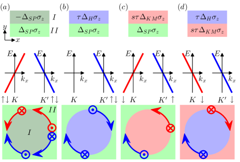
Figure 1: (a) - (d) The considered set of interfaces between insulating phases. The upper row shows the parameters related to each region, while the middle row depicts the corresponding dispersion of the emerging modes. The bottom row illustrates the hypothesis for the persistent currents in the closed loops inferred from the linear dispersion relations. Red (blue) lines depict the states belonging to the $K$ ($K^{\prime}$) valley, while the spin is denoted by the projection of the arrows.

An interface between any of the aforementioned insulating phases will support boundary modes. This can be shown by solving Eq. (1) for the geometry depicted in the upper row of Fig. 1. Note that in the domains $I$ and $II$ only a single mass term of the form $\Delta_{I/II}\sigma_{z}$ is used in Eq. (1). For instance, in case (c) $\Delta_{I}=s\tau\Delta_{KM}$ and $\Delta_{II}=\Delta_{SP}$. Then the evanescent modes, decaying exponentially away from the interface read

$$\Psi_{I/II}=e^{ik_{x}x}e^{\mp\kappa_{yI/II}y}\left[\begin{array}[]{c}1\\ \frac{\hbar v_{f}\left(\tau k_{x}\mp\kappa_{yI/II}\right)}{\Delta_{I/II}+E}\end{array}\right],$$ (2)

and we are interested in solutions $E=\pm\hbar v_{F}k_{x}$ with $\kappa_{yI/II}=\left|\Delta_{I/II}\right|/\hbar v_{F}$. Matching the wavefunctions at the boundary leads to the dispersion relations shown in the middle row of Fig. 1. These demonstrate chirality of the topological modes bound to the interface.qiao11 ; kane05b Unlike the cases in Figs. 1(c) and (d), the first two cases are spin degenerate.

Table 1: Summary of the numerical solutions. The symbol “$\times$” means that there are no allowed solutions, while the allowed modes are characterized by the corresponding angular momentum numbers $j$.

	$\uparrow K$	$\uparrow K^{\prime}$	$\downarrow K$	$\downarrow K^{\prime}$
(a)	$j>0$	$j<0$	$j>0$	$j<0$
(b)	$\times$	$j<0$	$\times$	$j<0$
(c)	$\times$	$j<0$	$j>0$	$\times$
(d)	$\times$	$\times$	$j<0$	$j<0$

We now present the main premise of our paper. Instead of straight interfaces, we consider circular ones, depicted in the bottom row of Fig. 1. The chirality of the boundary modes suggests that the angular momentum of the states in these loops must obey certain selection criteria depending on the particular phases in regions $I$ and $II$. For instance, in the cases (b) and (d) one would expect to see that only negative angular momentum valley and spin filtered states are allowed, respectively

To explore this explicitly, we solve the problem in polar coordinates, in which the Hamiltonian (1) reads

$$H=\left[\begin{array}[]{cc}\Delta_{I/II}&\pi^{-}\\ \pi^{+}&-\Delta_{I/II}\end{array}\right],$$ (3)

where $\pi^{\pm}=\tau\hbar v_{F}e^{\pm i\tau\phi}\left(-i\partial_{r}\pm\frac{\tau}{r}\partial_{\phi}\right)$. Because of the radial symmetry the total angular momentum $J_{z}=L_{z}+\tau\frac{\hbar}{2}\sigma_{z}$ is a good quantum number denoted by $j$,recher07 ; grujic11 and therefore the solution can be sought in the form

$$\Psi=e^{i(j-\tau/2)\phi}\left[\begin{array}[]{c}\chi_{A}(r)\\ e^{i\tau\phi}\chi_{B}(r)\end{array}\right].$$ (4)

The coupled system of equations reduces to the differential equation

$$\left[r^{2}\frac{d^{2}}{dr^{2}}+r\frac{d}{dr}-\frac{\Delta_{I/II}^{2}-E^{2}}{\hbar^{2}v_{F}^{2}}r^{2}-(j-\tau/2)^{2}\right]\chi_{A}=0.$$ (5)

Having in mind that we are interested in states lying within the bulk band gap $\Delta_{I/II}^{2}-E^{2}>0$, so that the solutions are the modified Bessel functions $I_{j-\tau/2}(r)$ and $K_{j-\tau/2}(r)$, which are exponentially divergent at $r\rightarrow\infty$ and $r=0$, respectively. The radially bound modes read

$$\Psi_{I}=e^{i(j-\tau/2)\phi}\left[\begin{array}[]{c}I_{j-\tau/2}\left(z_{I}(r)\right)\\ -i\tau e^{i\tau\phi}\frac{\sqrt{\Delta_{I}^{2}-E^{2}}}{\Delta_{I}+E}I_{j+\tau/2}\left(z_{I}(r)\right)\end{array}\right],$$ (6)

and

$$\Psi_{II}=e^{i(j-\tau/2)\phi}\left[\begin{array}[]{c}K_{j-\tau/2}\left(z_{II}(r)\right)\\ i\tau e^{i\tau\phi}\frac{\sqrt{\Delta_{II}^{2}-E^{2}}}{\Delta_{II}+E}K_{j+\tau/2}\left(z_{II}(r)\right)\end{array}\right],$$ (7)

where $z_{I/II}=\frac{\sqrt{\Delta_{I/II}^{2}-E^{2}}}{\hbar v_{F}}r$. Matching $\Psi_{I}$ and $\Psi_{II}$ at the interface $r=R$ results in the eigenvalue equation

$$\frac{\sqrt{\Delta_{II}^{2}-E^{2}}}{\Delta_{II}+E}K_{j+\tau/2}\left(z_{II}(R)\right)I_{j-\tau/2}\left(z_{I}(R)\right)$$

$$+\frac{\sqrt{\Delta_{I}^{2}-E^{2}}}{\Delta_{I}+E}I_{j+\tau/2}\left(z_{I}(R)\right)K_{j-\tau/2}\left(z_{II}(R)\right)=0,$$ (8)

which we solve numerically.

Our numerical results are summarized in Table 1 for four cases shown in Fig. 1. For those spin and valley flavors for which there exists a solution for a given interface we give the allowed angular momentum values, while the cases for which no solution is found are indicated by “$\times$”. Only results for positive energies are given, since the negative energy solutions are the same, albeit with opposite values of $j$. By inspecting Table 1 and comparing it with Fig. 1 one can see that the numerical results agree with the expectations deduced from the chirality of the topological modes. Namely, the angular momentum of the states bound to the loops not only display the expected orientation but are also: (a) valley-coupled, (b) valley-filtered, (c) spin-valley-filtered, and (d) spin-filtered.

In Fig. 2 the solid black lines are the numerically computed energies of the bound states for the radial interface corresponding to Fig. 1(a) for spin up in the $K$ valley. Note that for all the modes that are allowed, the set of energies is the same (only the angular momentum number $j$ varies), such that it suffices to show the spectrum for only one particular case. One can see that the larger loops can support states with larger $j$. Note also that, as a rule, there exists only one state for a given $j$. This is due to the exponential localization at the loop, which prevents oscillatory behavior in the radial direction and the emergence of a corresponding degree of freedom.

Interestingly, the energy curves follow a $1/R$ behavior with very high precision, a property also seen in states bound to the holes punched through topological insulators.shan11 It is relatively easy to obtain a good analytical fit of the energy levels using the following reasoning. Given the exponential localization of the modes near $r=R$, the loops effectively become 1D closed lines carrying states with pseudospin degree of freedom, described by $\psi$. Then, by requiring single-valuedness of $\psi$ upon one full revolution we must have $\psi(\phi+2\pi)=-e^{i\theta}\psi(\phi)$, where the contour is oriented counterclockwise. The minus sign comes from the spinorial nature of the state, and it forces the phase factor accumulated along the trajectory $\theta=\operatorname{sgn}(j)pL/\hbar$ ($L=2\pi R$ is the loop length) to be quantized in half integer multiples of $2\pi$. Denoting this half integer number by $j$, and recalling the dispersion of the topological modes $E=v_{F}p$, yields the following expression

$$E=\left|j\right|\frac{\hbar v_{F}}{R},$$ (9)

for the energy levels. They are shown in Fig. 2 by dashed red lines, and are in excellent agreement with the numerical results. Only small deviations are found for loops with small radius. This is to be expected, given that for small loops overlap of the wavefunction must occur, permitting tunneling of the modes between sections of the loop.

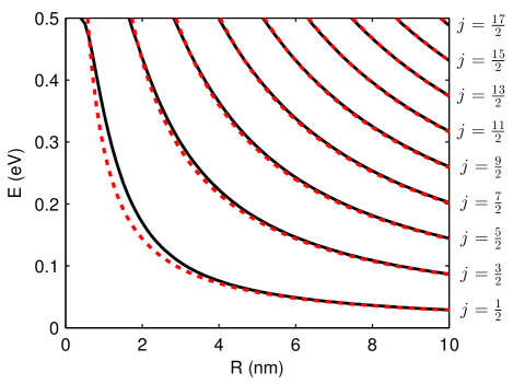
Figure 2: Variation of the numerically computed energy levels with radius $R$ (solid black lines), and the results from semiclassical quantization (dashed red lines) for the loop considered in Fig. 1(a). Here $\Delta_{SP}=0.5$ eV.

III The tight-binding method: generalization for arbitrarily shaped loops

Having analytically elucidated the chiral nature of the angular momenta, we now employ the TB method to study the behavior of the loops in a magnetic field. On the one hand, this is important because it can offer insights into intervalley scattering. Indeed, the most critical case is the setup (a), since valley flipping can cause back-reflection and mixing of the states, something not captured within the continuum approach. All the other loops are more robust, since either there are no counter-propagating states ((b) and (d)), or backscattering requires the simultaneous flipping of the valley and spin indices (setup (c)). On the other hand, the TB method will help us to resolve important details of the magnetic moments originating from the loops, even for noncircular geometries. The TB Hamiltonian that we employed reads

$$H=-t\sum_{\langle n,m\rangle}e^{i\varphi_{nm}}c^{\dagger}_{n}c_{m}+i\frac{s\Delta_{KM}}{3\sqrt{3}}\sum_{\langle\langle n,m\rangle\rangle}\nu_{nm}e^{i\varphi_{nm}}c^{\dagger}_{n}c_{m}.$$ (10)

We use $t=2.7$ eV for the hopping between nearest neighbor $p_{z}$ orbitals, while the second term is the SOC. Note that $\nu_{nm}=+1$ ($\nu_{nm}=-1$) if an electron makes a right (left) turn at the intermediate atom when hopping from site $m$ to site $n$. The Peierls term $\varphi_{nm}=-\frac{e}{\hbar}\int_{\mathbf{r_{m}}}^{\mathbf{r_{n}}}\mathbf{A}\cdot d\mathbf{l}$ accounts for the phase the electron acquires while traveling in the presence of the magnetic field. The staggered potential is simply added along the main diagonal of the Hamiltonian, like in the continuum model.

Our calculations were performed for a loop of radius $R=10$ nm contained within a larger circular quantum dot, with a $15$ nm radius, so that a proper decay of the topological modes is ensured. The results are shown by solid lines in Figs. 3(a) and (b) for the loop setups depicted in Figs. 1(a) and (c), respectively, as a function of the magnetic flux through the loop $\Phi=BR^{2}\pi$ in units of the flux quantum $\Phi_{0}=h/e$. For setup (a) the results are shown in black, since the TB model cannot resolve the two valleys, while for setup (c) (Fig. 3(b)) the valleys can be distinguished due to the additional spin polarization. In Fig. 3(a), for $B=0$ the majority of the levels are degenerate indicating the preservation of the valley index. Only a handful of levels (for instance those around $0.1$ eV) are offset by an equally small amount in the opposite directions with respect to the continuum solutions. This behavior indicates that such states are susceptible to intervalley scattering, causing bonding and anti-bonding states. As the magnetic field is turned on, the remaining valley degeneracy is lifted due to the opposite magnetic moments (see below). Moreover, an anticrossing behavior occurs at energies where intervalley scattering is prominent, resulting in an Aharonov-Bohm-like pattern of the curves. On the other hand, for the setup (c), such scattering is impossible in the TB picture due to the absence of spin-flipping terms in the Hamiltonian, as demonstrated by Fig. 3(b). Consequently, the spin up in the $K^{\prime}$ valley (solid blue curve), with a magnetic moment oriented along the magnetic field, and the spin down in the $K$ valley (solid red curve) with the opposite orientation of the magnetic moment are independent of each other, and experience a rigid, linear, decrease and an increase in energy, respectively.

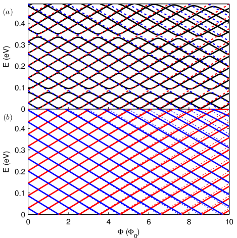
Figure 3: The magnetic field dependence of the energy spectrum for the loops depicted in (a) Fig. 1(a) and (b) Fig. 1(c). We used $\Delta_{SP}=\Delta_{KM}=0.5$ eV. Solid curves depict the TB results, while the dashed lines are given by Eq. (11). Red (blue) depicts the states belonging to the $K$ ($K^{\prime}$) valley.

In order to capture the behavior of the topological modes in the presence of a magnetic field, we again consider the phase change upon a single rotation around the loop. Now, due to the magnetic field an additional phase factor of the form (assuming $B$ is constant inside the loop) $-\frac{e}{\hbar}\oint\mathbf{A}\cdot d\mathbf{l}=-\frac{e}{\hbar}BS$ appears, where $S$ is the loop area. As before, $\theta$ must be a half integer multiple of $2\pi$, yielding

$$E=\left|j\right|\frac{hv_{F}}{L}+\operatorname{sgn}(j)\frac{ev_{F}}{L}SB.$$ (11)

These levels are depicted by dashed curves in Fig. 3 and show excellent agreement with the TB results, with small deviations at very large magnetic fields.latyshev14 Note that the change in energy due to magnetic field can be captured entirely by the classical formula for the energy of a closed current contour given by $-\mu B$. Besides the area of the loop, the magnetic moment of a classical contour $\mu=IS$ depends on the current due to one topological mode $I=\operatorname{sgn}(j)(-e)/T$, where $T=\operatorname{sgn}(j)(-e)v_{F}/L$ is the period, and matches the one in expression Eq. (11) exactly.

Most importantly, note that Eq. (11) is written in a general form, without specifying the precise shape of the loop, since it depends only on its length and area. In fact, we have verified numerically by using the TB method that the above formula accurately predicts the energies and magnetic moments of the states in loops with arbitrary shape. In particular, in Fig 4 we show the results for the same two setups as in Fig. 3, but for a elliptic, hexagonal zigzag and hexagonal armchair loops. Note that $j$ does not denote the total angular momentum now, due to the lack of rotational symmetry. However, it is still required to be a half-integer, while its sign reflects the orientation of the chiral current. For the elliptic loop (Figs. 4(a) and (b)) we have used $R_{1}=5$ nm, $R_{2}=15$ nm, $S=R_{1}R_{2}\pi$, and for the loop length we have used the approximation of the form

$$L=\pi(R_{1}+R_{2})\left(1+\frac{3d}{10+\sqrt{4-3d}}\right),$$ (12)

where $d=\left(R_{1}-R_{2}\right)^{2}/\left(R_{1}+R_{2}\right)^{2}$. The hexagonal loops are distinguished by the number of zigzag ($N_{ZG}$) or armchair ($N_{AC}$) segments along one edge. The loop length ($L=6l$) and area ($S=6l^{2}\sqrt{3}/4$), depend on the length of one side of the hexagon $l_{ZG}=N_{ZG}\sqrt{3}a$ ($l_{AC}=(3N_{AC}-2)a$), where $a$ is the nearest neighbor distance. The results depicted in Figs. 4(c) and (d), and (e) and (f) are for $N_{ZG}=42$ and $N_{AC}=25$, respectively. All the loops are surrounded by a region large enough to ensure the decay of the topological modes.

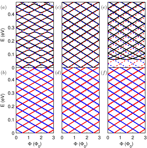
Figure 4: The same as in Fig. 3, but for an elliptic loop ((a) and (b)), hexagonal zigzag loop ((c) and (d)), and hexagonal armchair loop ((e) and (f)).

On the one hand, for setup (c) (where counterpropagating states belong to opposite spins, lower panels), it can be seen that regardless of the shape, the persistent current is robust, and that Eq. (11) predicts the energy levels with great accuracy. The very small mismatch that appears we attribute to the fact that the sharp turns and corners can effectively reduce the loop length and area due to tunneling, and hence cause some deviation from the expected behavior. On the other hand, the spectrum of setup (a) (upper panels) shows that intervalley scattering is geometry dependent, as one would expect, although Eq. (11) still provides a very good approximation for the results in general. While elliptic loops display stronger intervalley scattering and subsequent hybridization than the circular loops, intervalley scattering in zigzag hexagonal loops is practically nonexistent. Finally, in armchair hexagonal loops a gap is opened for low-energy chiral states, a situation resembling the appearance of mass barriers in graphene quantum rings.roman13 Remarkably, away from this energy region a behavior indicating chirality preservation is observed, although the valley degree of freedom is ill-defined in this structure. Therefore, to a good approximation one can say that the electronic and magnetic properties of these loops are largely independent on the precise details of the edges near the interface. This is unlike the case in regular graphene nanorings, where geometry and boundary of the rings can hinder the fidelity of the simplified 1D models,costa14 with the main reason for this contrast being the exponential localization of the topological states.

IV Discussion and the conclusion

Now we consider the possible applications of these effects. By controlling the valley population separately in the setup (a) for example (in loops with well preserved valley index), one could in turn control the total magnetization of the loop, since all orbits within a given valley have the same orientation of the persistent current. In setup (b) the $K$ valley does not host topological boundary modes, unlike the $K^{\prime}$ valley, where the persistent current has the same orientation regardless of spin. Hence, these particular loops should be inherently magnetic. Alternatively, in setup (c) one can control the total magnetization by adjusting the spin or spin-valley populations.grujic14a Finally the loops in setup (d) not only display nonzero magnetism, as those in setup (b), they have the additional benefit that the allowed topological modes have their spins aligned, which can contribute to the overall magnetic moment. Therefore, these loops have a tremendous potential for the design of novel magnetic structures and devices. One can imagine an array of these loops laid out in a pattern designed to suit a particular application. Moreover, since the states racing along these loops are exponentially localized in the radial direction the array can be densely packed, enabling the creation of hybrid magnets.

Before we conclude, let us reflect on the practical issues concerning the real materials that are required to create these structures. On the one hand, it is well known that inversion symmetry can be broken by layering graphene with boron-nitride, which has a naturally occurring staggered potential since it’s sublattices are composed out of different atomic species.hunt13 Moreover, in-plane heterostructures of graphene and boron-nitride have been demonstrated in recent experiments.liu13 ; liu14 In particular, in Ref. liu13, the authors presented a matrix array of circular graphene dots embedded in boron-nitride. Since the resulting structure was transferable, one can imagine layering it with a substrate which would enhance SOC in graphene, such as ${\rm WS}_{2}$ for instance,avsar14 thereby creating a macroscopic pattern of chiral closed-contour currents of the type shown in Fig. 1(c).

On the other hand, given the buckled lattice structure of silicene, germanene and stanene,cahangirov09 ; liu11 ; xu13 breaking of the inversion symmetry can be realized by external gates, while relatively heavy constituent atoms ensure nonzero SOC. Patterning gates on top of them could likewise induce chiral persistent currents described in this paper, making them detectable for instance by magnetic force microscopy. Additionally, there are theoretical proposals for inducing the QAH effect in graphene and silicene, although experimental validation is still lacking.kitagawa11 ; qiao14b ; barnea12 ; wright13 ; zhang13 ; kaloni14

As we have shown, the larger the bulk band gap and the loop radius, the larger the magnetization will be. However, large loops and inherent spin and valley relaxation mechanisms will inevitably lead to scattering, spoiling the effect to a certain degree. Nevertheless, no amount of scattering can change the orientation of the persistent current, which is related to the topology of the surrounding band structures, and the emptied states should quickly become repopulated. Note that, while the interplay of orbital magnetism emerging in insulating Dirac systems,xiao07 ; zhang11 ; grujic14b and the magnetism of topological-state loops remains to be explored, the main obstacle for realizing this effect is most likely related to the size of the bulk band gaps. This can not only restrict the amount of persistent current supported by the loops, but more importantly limit the temperature range of applicability.

To summarize, we investigated the behavior of electronic states bound to looped interfaces between insulating phases of distinct topologies. These structures can be a source of magnetic moments due to persistent currents flowing along the interfaces. The chirality of the states bound to these loops manifests as a chirality in the angular momentum and the corresponding magnetic moments. We have shown that a simple 1D model captures both the qualitative and the quantitative behavior of the electrons. By calculating energy levels and magnetic moments in elliptic, hexagonal zigzag, and hexagonal armchair loops, it was shown that the model’s validity extends to noncircular loops as well. Because of the intimate link between the magnetic moments and spin and valley degrees of freedom, novel magnetic structures and devices can be envisioned.

- (1) I. Martin, Y. M. Blater and A. F. Morpurgo, Phys. Rev. Lett. 100, 036804 (2008).
- (2) Z. Qiao, J. Jung, Q. Niu, and A. H. MacDonald, Nano Lett. 11, 3453 (2011).
- (3) Z. Qian, J. Liu, L. Fu and J. Li, Science 346, 1344 (2014).
- (4) H. Pan, X. Li, F. Zhang, and S. A. Yang, arXiv:1501.00114v1.
- (5) X.-L. Qi and S.-C. Zhang, Rev. Mod. Phys. 83, 1057 (2011).
- (6) C. L. Kane and E. J. Mele, Phys. Rev. Lett. 95, 146802 (2005).
- (7) C. L. Kane and E. J. Mele, Phys. Rev. Lett. 95, 226801 (2005).
- (8) B. A. Bernevig and S.-C. Zhang, Phys. Rev. Lett. 96, 106802 (2006).
- (9) M. Zarenia, J. M. Pereira Jr., G. A. Farias, and F. M. Peeters, Phys. Rev. B 84, 125451 (2011).
- (10) M. Zarenia, O. Leenaerts, B. Partoens, and F. M. Peeters, Phys. Rev. B 86, 085451 (2012).
- (11) T. Tudorovskiy and M. I. Katsnelson, Phys. Rev. B 86, 045419 (2012).
- (12) J. Jung, Z. Qiao, Q. Niu, and A. H. MacDonald, Nano Lett. 12, 2936 (2012).
- (13) Z. Qiao, J. Jung, C. Lin, Y. Ren, A. H. MacDonald, and Q. Niu, Phys. Rev. Lett. 112, 206601 (2014).
- (14) Y. Kim, K. Choi, J. Ihm, and H. Jin, Phys. Rev. B 89, 085429 (2014).
- (15) D. S. L. Abergel, J. M. Edge, and A. V. Balatsky, New J. Phys. 16, 065012 (2014).
- (16) S. K. Wang, J. Wang, and K. S. Chan, New J. Phys. 16, 045015 (2014).
- (17) S. Rachel and M. Ezawa, Phys. Rev. B 89, 195303 (2014).
- (18) W.-Y. Shan, J. Lu, H.-Z. Lu, and S.-Q. Shen, Phys. Rev. B 84, 035307 (2011).
- (19) F. D. M. Haldane, Phys. Rev. Lett. 61, 2015 (1988).
- (20) P. Recher, B. Trauzettel, A. Rycerz, Y. M. Blanter, C. W. J. Beenakker, and A. F. Morpurgo, Phys. Rev. B 76, 235404 (2007).
- (21) M. Grujić, M. Zarenia, A. Chaves, M. Tadić, G. A. Farias, and F. M. Peeters, Phys. Rev. B 84, 205441 (2011).
- (22) Non-topological Tamm-Dirac edge states, appearing near graphene nanoholes, also give rise to these levels, impacting the magnetotransport measurements, see: Yu I. Latyshev, A. P. Orlov, V. A. Volkov, V. V. Enaldiev, I. V. Zagorodnev, O. F. Vyvenko, Yu V. Petrov, and P. Monceau, Nat. Commun. 4, 7578 (2014).
- (23) I. Romanovsky, C. Yannouleas, and U. Landman, Phys. Rev. B 87, 165431 (2013).
- (24) D. R. da Costa, A. Chaves, M. Zarenia, J. M. Pereira Jr., G. A. Farias, and F. M. Peeters, Phys. Rev. B 89, 075418 (2014).
- (25) M. M. Grujić, M. Ž Tadić, and F. M. Peeters, Phys. Rev. Lett. 113, 046601 (2014).
- (26) B. Hunt, J. D. Sanchez-Yamagishi, A. F. Young, M. Yankowitz, B. J. LeRoy, K. Watanabe, T. Taniguchi, P. Moon, M. Koshino, P. Jarillo-Herrero, and R. C. Ashoori, Science 340, 1427 (2013).
- (27) Z. Liu, L. Ma, G. Shi, W. Zhou, Y. Gong, S. Lei, X. Yang, J. Zhang, J. Yu, K. P. Hackenberg, A. Babakhani, J.-C. Idrobo, R. Vajtai, J. Lou, and P. M. Ajayan, Nature Nanotech. 8, 119 (2013).
- (28) L. Liu, J. Park, D. A. Siegel, K. F. McCarty, K. W. Clark, W. Deng, L Basile, J.-C. Idrobo, A.-P. Li, and G. Gu, Science 343, 163 (2014).
- (29) A. Avsar, J. Y. Tan, T. Taychatanapat, J. Balakrishnan, G.K.W. Koon, Y. Yeo, J. Lahiri, A. Carvalho, A. S. Rodin, E.C.T. O’Farrell, G. Eda, A. H. Castro Neto, and B. Ozyilmaz, Nat. Commun. 5, 4875 (2014).
- (30) S. Cahangirov, M. Topsakal, E. Aktürk, H. Şahin, and S. Ciraci, Phys. Rev. Lett. 102, 236804 (2009).
- (31) Cheng-Cheng Liu, Wanxiang Feng, and Yugui Yao, Phys. Rev. Lett. 107, 076802 (2011).
- (32) Y. Xu, B. Yan, H. J. Zhang, J. Wang, G. Xu, P. Tang, W. Duan, and S. C. Zhang, Phys. Rev. Lett. 111, 136804 (2013).
- (33) T. Kitagawa, T. Oka, A. Brataas, L. Fu, and E Demler, Phys. Rev. B 84, 235108 (2011).
- (34) Z. Qiao, W. Ren, H. Chen, L. Bellaiche, Z. Zhang, A. H. MacDonald, and Q. Niu, Phys. Rev. Lett. 112, 116404 (2014).
- (35) T. Pereg-Barnea and G. Refael, Phys. Rev. B 85, 075127 (2012).
- (36) A. R. Wright, Sci. Rep. 3, 2736 (2013).
- (37) X.-L. Zhang, L.-F. Liu, and W.-M. Liu, Sci. Rep. 3, 2908 (2013).
- (38) T. P. Kaloni, N. Singh, and U. Schwingenschlögl, Phys. Rev. B 89, 035409 (2014).
- (39) D. Xiao, W. Yao, and Q. Niu, Phys. Rev. Lett. 99, 236809 (2007).
- (40) F. Zhang, J. Jung, G. A. Fiete, Q. Niu, and A. H. MacDonald, Phys. Rev. Lett, 106, 156801 (2011).
- (41) M. M. Grujić, M. Ž. Tadić, and F. M. Peeters, Phys. Rev. B 90, 205408 (2014).