When Social Influence Meets Item Inference
Abstract
Research issues and data mining techniques for product recommendation and viral marketing have been widely studied. Existing works on seed selection in social networks do not take into account the effect of product recommendations in e-commerce stores. In this paper, we investigate the seed selection problem for viral marketing that considers both effects of social influence and item inference (for product recommendation). We develop a new model, Social Item Graph (SIG), that captures both effects in form of hyperedges. Accordingly, we formulate a seed selection problem, called Social Item Maximization Problem (SIMP), and prove the hardness of SIMP. We design an efficient algorithm with performance guarantee, called Hyperedge-Aware Greedy (HAG), for SIMP and develop a new index structure, called SIG-index, to accelerate the computation of diffusion process in HAG. Moreover, to construct realistic SIG models for SIMP, we develop a statistical inference based framework to learn the weights of hyperedges from data. Finally, we perform a comprehensive evaluation on our proposals with various baselines. Experimental result validates our ideas and demonstrates the effectiveness and efficiency of the proposed model and algorithms over baselines.
1 Introduction
The ripple effect of social influence [3] has been explored for viral marketing via online social networks. Indeed, studies show that customers tend to receive product information from friends better than advertisements on traditional media [18]. To explore the potential impact of social influence, many research studies on seed selection, i.e., selecting a given number of influential customers to maximize the spread of social recommendation for a product, have been reported [6, 16].111All the top 5 online retailers, including Amazon, Staples, Apple, Walmart, and Dell, are equipped with sophisticated recommendation engines. They also support viral marketing by allowing users to share favorite products in Facebook. However, these works do not take into account the effect of product recommendations in online e-commerce stores. We argue that when a customer buys an item due to the social influence (e.g., via Facebook or Pinterest), there is a potential side effect due to the item inference recommendations from stores.222In this paper, we refer product/item recommendation based on associations among items inferred from purchase transactions as item inference recommendation. For example, when Alice buys a DVD of “Star War” due to the recommendation from friends, she may also pick up the original novel of the movie due to an in-store recommendation, which may in turn trigger additional purchases of the novel among her friends. To the best of our knowledge, this additional spread introduced by the item inference recommendations has not been considered in existing research on viral marketing.
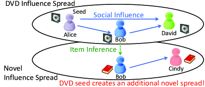
Figure 1 illustrates the above joint effects in a toy example with two products and four customers, where a dash arrow represents the association rule behind the item inference recommendation, and a solid arrow denotes the social influence between two friends upon a product. In the two separate planes corresponding to DVD and novel, social influence is expected to take effect on promoting interests in (and potential purchases of) the DVD and novel, respectively. Meanwhile, the item inference recommendation by the e-commerce store is expected to trigger sales of additional items. Note that the association rules behind item inference are derived without considering the ripple effect of social influence. In the example, when Bob buys the DVD, he may also buy the novel due to the item inference recommendation. Moreover, he may influence Cindy to purchase novel. However, the association rules behind item inference are derived without considering the ripple effect of social influence. On the other hand, to promote the movie DVD, Alice may be selected as a seed for a viral marketing campaign, hoping to spread her influence to Bob and David to trigger additional purchases of the DVD. Actually, due to the effect of item inference recommendation, having Alice as a seed may additionally trigger purchases of the novel by Bob and Cindy. This is a factor that existing seed selection algorithms for viral marketing do not account for.
We argue that to select seeds for maximizing the spread of product information to a customer base (or maximizing the sale revenue of products) in a viral marketing campaign, both effects of item inference and social influence need to be considered. To incorporate both effects, we propose a new model, called Social Item Graph (SIG) in form of hyperedges, for capturing “purchase actions” of customers on products and their potential influence to trigger other purchase actions. Different from the conventional approaches [6, 16] that use links between customers to model social relationship (for viral marketing) and links between items to capture the association (for item inference recommendation), SIG represents a purchase action as a node (denoted by a tuple of a customer and an item), while using hyperedges among nodes to capture the influence spread process used to predict customers’ future purchases. Unlike the previous influence propagation models [6, 16] consisting of only one kind of edges connecting two customers (in social influence), the hyperedges in our model span across tuples of different customers and items, capturing both effects of social influence and item inference.
Based on SIG, we formulate the Social Item Maximization Problem (SIMP) to find a seed set, which consists of selected products along with targeted customers, to maximize the total adoptions of products by customers. Note that SIMP takes multiple products into consideration and targets on maximizing the number of products purchased by customers.333SIMP can be extended to a weighted version with different profits from each product. In this paper, we focus on maximizing the total sales. SIMP is a very challenging problem, which does not have the submodularity property. We prove that SIMP cannot be approximated within with any , where is the number of nodes in SIMP, i.e., SIMP is extremely difficult to approximate with a small ratio because the best approximation ratio is almost .444While there is no good solution quality guarantee for the worst case scenario, we empirically show that the algorithm we developed achieves total adoptions on average comparable to optimal results.
To tackle SIMP, two challenges arise: 1) numerous combinations of possible seed nodes, and 2) expensive on-line computation of influence diffusion upon hyperedges. To address the first issue, we first introduce the Hyperedge-Aware Greedy (HAG) algorithm, based on a unique property of hyperedges, i.e., a hyperedge requires all its source nodes to be activated in order to trigger the purchase action in its destination node. HAG selects multiple seeds in each seed selection iteration to further activate more nodes via hyperedges.555A hyperedge requires all its source nodes to be activated to diffuse its influence to its destination node. To address the second issue, we exploit the structure of Frequent Pattern Tree (FP-tree) to develop SIG-index as an compact representation of SIG in order to accelerate the computation of activation probabilities of nodes in online diffusion.
Moreover, to construct realistic SIG models for SIMP, we also develop a statistical inference based framework to learn the weights of hyperedges from logs of purchase actions. Identifying the hyperedges and estimating the corresponding weights are major challenges for constructing of a SIG due to data sparsity and unobservable activations. To address these issues, we propose a novel framework that employs smoothed expectation and maximization algorithm (EMS) [20], to identify hyperedges and estimate their values by kernel smoothing.
Our contributions of this paper are summarized as follows.
-
•
We observe the deficiencies in existing techniques for item inference recommendation and seed selection and propose the Social Item Graph (SIG) that captures both effects of social influence and item inference in prediction of potential purchase actions.
-
•
Based on SIG, we formulate a new problem, called Social Item Maximization Problem (SIMP), to select the seed nodes for viral marketing that effectively facilitates the recommendations from both friends and stores simultaneously. In addition, we analyze the hardness of SIMP.
-
•
We design an efficient algorithm with performance guarantee, called Hyperedge-Aware Greedy (HAG), and develop a new index structure, called SIG-index, to accelerate the computation of diffusion process in HAG.
-
•
To construct realistic SIG models for SIMP, we develop a statistical inference based framework to learn the weights of hyperedges from data.
-
•
We conduct a comprehensive evaluation on our proposals with various baselines. Experimental result validates our ideas and demonstrates the effectiveness and efficiency of the proposed model and algorithms over baselines.
The rest of this paper is organized as follows. Section 2 reviews the related work. Section 3 details the SIG model and its influence diffusion process. Section 4 formulates SIMP and designs new algorithms to efficiently solve the problem. Section 5 describes our approach to construct the SIG. Section 6 reports our experiment results and Section 7 concludes the paper.
2 Related Work
To discover the associations among purchased items, frequent pattern mining algorithms find items which frequently appear together in transactions [2]. Some variants, such as closed frequent patterns mining [19], maximal frequent pattern mining [15], have been studied. However, those existing works, focusing on unveiling the common shopping behaviors of individuals, disregard the social influence between customers [26]. On the other hand, it has been pointed out that items recommended by item inference may have been introduced to users by social diffusion [25]. In this work, we develop a new model and a learning framework that consider both the social influence and item inference factors jointly to derive the association among purchase actions of customers. In addition, we focus on seed selection for prevalent viral marketing by incorporating the effect of item inference.
With a great potential in business applications, social influence diffusion in social networks has attracted extensive interests recently [6, 16]. Learning algorithms for estimating the social influence strength between social customers have been developed [9, 17]. Based on models of social influence diffusion, identifying the most influential customers (seed selection) is a widely studied problem [6, 16]. Precisely, those studies aim to find the best initial seed customers to target on in order to maximize the population of potential customers who may adopt the new product. This seed selection problem has been proved as NP-hard [16]. Based on two influence diffusion models, Independent Cascade (IC) and Linear Threshold (LT), Kempe et al. propose a approximation greedy algorithm by exploring the submodularity property under IC and LT [16]. Some follow-up studies focus on improving the efficiency of the greedy algorithm using various spread estimation methods, e.g., MIA[6] and TIM+[23]. However, without considering the existence of item inference, those algorithms are not applicable to SIMP. Besides the IC and LT model, Markov random field has been used to model social influence and calculate expected profits from viral marketing [8]. Recently, Tang et al. proposed a Markov model based on “confluence”, which estimates the total influence by combining different sources of conformity [22]. However, these studies only consider the diffusion of a single item in business applications. Instead, we incorporate item inference in spread maximization to estimate the influence more accurately.
3 Social Item Graph Model
Here we first present the social item graph model and then introduce the diffusion process in the proposed model.
3.1 Social Item Graph
We aim to model user purchases and potential activations of new purchase actions from some prior. We first define the notions of the social network and purchase actions.
Definition 1
A social network is denoted by a directed graph where contains all the nodes and contains all the directed edges in the graph. Accordingly, a social network is also referred to as a social graph.
Definition 2
Given a list of commodity items and a set of customers , a purchase action (or purchase for short), denoted by where is a customer, and is an item, refers to the purchase of item by customer .
Definition 3
An purchase log is a database consisting of all the purchase actions in a given period of time.
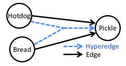
Association-rule mining (called item inference in this paper) has been widely exploited to discover correlations between purchases in transactions. For example, the rule obtained from the transactions of a supermarket indicates that if a customer buys hotdogs and bread together, she is likely to buy pickles. To model the above likelihood, the confidence [11] of a rule is the proportion of the transactions that have hotdogs and bread also include pickles. It has been regarded as the conditional probability that a customer buying both hotdogs and bread would trigger the additional purchase of pickles. To model the above rule in a graph, a possible way is to use two separate edges (see Figure 2; one from hotdog to pickle, and the other from bread to pickle, respectively), while the probability associated with each of these edges is the confidence of the rule. In the above graph model, however, either one of the hotdog or bread may trigger the purchase of pickle. This does not accurately express the intended condition of purchasing both the hotdog and bread. By contrast, the hyperedges in Graph Theory, by spanning multiple source nodes and one destination node, can model the above association rule (as illustrated in Figure 2). The probability associated with the hyperedge represents the likelihood of the purchase action denoted by the destination node when all purchase actions denoted by source nodes have happened.
On the other hand, in viral marketing, the traditional IC model activates a new node by the social influence probabilities associated with edges to the node. Aiming to capture both effects of item inference and social influence. We propose a new Social Item Graph (SIG). SIG models the likelihood for a purchase (or a set of purchases) to trigger another purchase in form of hyperedges, which may have one or multiple source nodes leading to one destination node. We define a social item graph as follows.
Definition 4
Given a social graph of customers and a commodity item list , a social item graph is denoted by , where is a set of purchase actions and is a set of hyperedges over . A node is denoted as , where and . A hyperedge is of the following form:
where is in the neighborhood of in , i.e., .666Notice that when , the hyperedge represents the item inference of item . On the other hand, when , it becomes the social influence of user on .
Note that the conventional social influence edge in a social graph with one source and one destination can still be modeled in an SIG as a simple edge associated with a corresponding influence probability. Nevertheless, the influence probability from a person to another can vary for different items (e.g., a person’s influence on another person for cosmetics and smartphones may vary.). Moreover, although an SIG may model the purchases more accurately with the help of both social influence and item inference, the complexity of processing an SIG with hyperedges is much higher than simple edges in the traditional social graph that denotes only social influence.777To solve this issue, one approach is to transform a SIG with hyperedges to a graph without hyperedges, by replacing a hyperedge with multiple simple edges connecting to the sources and destinations, or by aggregating the source nodes and destination nodes into two nodes, respectively. Nevertheless, as to be shown in Section 4, the above strategies do not work. Also, a destination node can be activated only if all source nodes of the hyperedge are activated (see Section 3.2).
For simplicity, let and (i.e., the symbols in Typewriter style) represent the nodes and in SIG for the rest of this paper. We also denote a hyperedge as , where is a set of source nodes and is the destination node. Let the associated edge weight be , which represents the activation probability for to be activated if all source nodes in are activated. Note that the activation probability is for one single hyperedge . Other hyperedges sharing the same destination may have different activation probabilities. For example, part of the source nodes in a hyperedge can still activate , e.g., by with a different hyperedge with its own activation probability.
3.2 Diffusion Process in Social Item Graph
Next we introduce the diffusion process in SIG, which is inspired by the probability-based approach behind Independent Cascade (IC) to captures the word-of-mouth behavior in the real world [6].888Notice that diffusion process in SIG is based on IC model since it only requires one diffusion probability parameter associated to each edge whereas LT model requires both influence degree of each edge and an influence threshold for each node. Moreover, several variants of IC model have been proposed [5, 4]. However, they focus on modeling the diffusion process between users, such as aspect awareness [5], which is not suitable for social item graph since the topic is embedded in each SIG node. This diffusion process fits the item inferences captured in an SIG naturally, as we can derive conditional probabilities on hyperedges to describe the trigger (activation) of purchase actions on a potential purchase.
The diffusion process in SIG starts with all nodes inactive initially. Let S denote a set of seeds (purchase actions). Let a node be a seed. It immediately becomes active. Given all the nodes in a source set at iteration , if they are all active at iteration , a hyperedge has a chance to activate the inactive with probability . Each node can be activated once, but it can try to activate other nodes multiple times, one for each incident hyperedges. For the seed selection problem that we target on, the total number of activated nodes represents the number of items adopted by customers (called total adoptions for the rest of this paper).
4 Social Item Maximization
Upon the proposed Social Item Graph (SIG), we now formulate a new seed selection problem, called Social Item Maximization Problem (SIMP), that selects a set of seed purchase actions to maximize potential sales or revenue in a marketing campaign. In Section 5, we will describe how to construct the SIG from purchase logs by a machine learning approach.
Definition 5
Given a seed number , a list of targeted items , and a social item graph , SIMP selects a set S of seeds in such that , the total adoption function of S, is maximized.
Note that a seed in SIG represents the adoption/purchase action of a specific item by a particular customer. The total adoption function represents the total number of product items () purchased. By assigning prices to products and costs to the selected seeds, an extension of SIMP is to maximize the total revenue subtracted by the cost.
Here we first discuss the challenges in solving SIMP before introducing our algorithm. Note that, for the influence maximization problem based on the IC model, Kempe et al. propose a approximation algorithm [16], thanks to the submodularity in the problem. Unfortunately, the submodularity does not hold for the total adoption function in SIMP. Specifically, if the function satisfies the submodularity, for any node i and any two subsets of nodes and where , should hold. However, a counter example is illustrated below.


Example 1
Consider an SIMP instance with a customer and five items in Figure 4. Consider the case where , , and i corresponds to node . For seed sets , , and , , , , and . Thus, . Hence, the submodularity does not hold.
Since the submodularity does not exist in SIMP, the approximation ratio of the greedy algorithm in [16] does not hold. Now, an interesting question is how large the ratio becomes. Example 2 shows an SIMP instance where the greedy algorithm performs poorly.
Example 2
Consider an example in Figure 4, where nodes , ,…, all have a hyperedge with the probability as 1 from the same sources , ,…, , and is an arbitrarily small edge probability . The greedy algorithm selects one node in each iteration, i.e., it selects , … as the seeds with a total adoption . However, the optimal solution actually selects , ,…, as the seeds and results in the total adoption . Therefore, the approximation ratio of the greedy algorithm is at least , which is close to for a large , where could approach in the worst case.


One may argue that the above challenges in SIMP may be alleviated by transforming into a graph with only simple edges, as displayed in Figure 5, where the weight of every with can be set independently. However, if a source node of v is difficult to activate, the probability for v to be activated approaches zero in Figure 5 (a) due to . However, in Figure 5 (b), the destination v is inclined to be activated by sources in U, especially when U is sufficiently large. Thus, the idea of graph transformation does not work.
4.1 Hyperedge-Aware Greedy (HAG)
Here, we propose an algorithm for SIMP, Hyperedge-Aware Greedy (HAG), with performance guarantee. The approximation ratio is proved in Section 4.3. A hyperedge requires all its sources activated first in order to activate the destination. Conventional single node greedy algorithms perform poorly because hyperedges are not considered. To address this important issue, we propose Hyperedge-Aware Greedy (HAG) to select multiple seeds in each iteration.
A naive algorithm for SIMP would examine, combinations are involved to choose seeds. In this paper, as multiple seeds tend to activate all source nodes of a hyperedge in order to activate its destination, an effective way is to consider only the combinations which include the source nodes of any hyperedge. We call the source nodes of a hyperedge as a source combination. Based on this idea, in each iteration, HAG includes the source combination leading to the largest increment on total adoption divided by the number of new seeds added in this iteration. Note that only the source combinations with no more than sources are considered. The iteration continues until seeds are selected. Note that HAG does not restrict the seeds to be the source nodes of hyperedges. Instead, the source node of any simple edge in SIG is also examined.
Complexity of HAG. To select seeds, HAG takes at most rounds. In each round, the source combinations of hyperedges are tried one by one, and the diffusion cost is , which will be analyzed in Section 4.2. Thus, the time complexity of HAG is .
4.2 Acceleration of Diffusion Computation
To estimate the total adoption for a seed set, it is necessary to perform Monte Carlo simulation based on the diffusion process described in Section 3.2 for many times. Finding the total adoption is very expensive, especially when a node v can be activated by a hyperedge with a large source set U, which indicates that there also exist many other hyperedges with an arbitrary subset of U as the source set to activate v. In other words, enormous hyperedges need to be examined for the diffusion on an SIG. It is essential to reduce the computational overhead. To address this issue, we propose a new index structure, called SIG-index, by exploiting FP-Tree [11] to pre-process source combinations in hyperedges in a compact form in order to facilitate efficient derivation of activation probabilities during the diffusion process.
The basic idea behind SIG-index is as follows. For each node with the set of activated in-neighbors in iteration , if has not been activated before , the diffusion process will try to activate via every hyperedge where the last source in has been activated in iteration . To derive the activation probability of a node from the weights of hyperedges associated with , we first define the activation probability as follows.
Definition 6
The activation probability of at is
where and denote the set of active neighbors of in iteration and , respectively.
The operations on an SIG-index occur two phases: Index Creation Phase and Diffusion Processing Phase. As all hyperedges satisfying Definition 6 must be accessed, the SIG-index stores the hyperedge probabilities in Index Creation Phase. Later, the SIG-index is updated in Diffusion Processing Phase to derive the activation probability efficiently.
Index Creation Phase. For each hyperedge , we first regard each source combination as a transaction to build an FP-tree [11] by setting the minimum support as 1. As such, forms a path from the root in the FP-tree to node in . Different from the FP-Tree, the SIG-index associates the probability of each hyperedge with the last source node in .999For ease of explanation, we assume the order of nodes in the SIG-index follows the ascending order of subscript. Initially the probability associated with the root is 0. Later the the SIG-index is updated during the diffusion process. Example 3 illustrates the SIG-index created based on an SIG.
Example 3
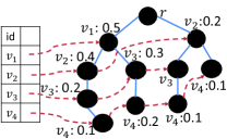
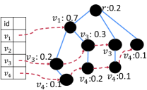
Consider an SIG graph with five nodes, -, and nine hyperedges with their associated probabilities in parentheses:101010For simplicity, the hyperedges in this example only have as the destination. (0.5), (0.4), (0.2), (0.1), (0.3), (0.2), (0.2), (0.1), (0.1). Figure 6 (a) shows the SIG-index initially created for node .
Diffusion Processing Phase. The activation probability in an iteration is derived by traversing the initial SIG-index, which takes time. However, a simulation may iterate a lot of times. To further accelerate the traversing process, we adjust the SIG-index for the activated nodes in each iteration. More specifically, after a node is activated, accessing an hyperedge with becomes easier since the number remaining inactivated nodes in is reduced. Accordingly, SIG-index is modified by traversing every vertex labeled as on the SIG-index in the following steps. 1) If is associated with a probability , it is crucial to aggregate the old activation probabilities of and of its parent , and update activation probability associated with as , since the source combination needed for accessing the hyperedges associated with and becomes the same. The aggregation is also performed when is . 2) If has any children , the parent of is changed to be , which removes the processed from the index. 3) After processing every node in the SIG-index, we obtain the activation probability of in the root . After the probability is accessed for activating v, the probability of is reset to 0 for next iteration.
Example 4
Consider an example with activated in an iteration. To update the SIG-index, each vertex in Figure 6 (a) is examined by traversing the linked list of . First, the left vertex with label is examined. SIG-index reassigns the parent of ’s child (labeled as ) to the vertex labeled as , and aggregate the probability 0.4 on the and 0.5 on vertex , since the hyperedge can be accessed if the node is activated later. The probability of becomes . Then the right vertex with label is examined. The parent of its two children is reassigned to the root . Also, the probability of itself (0.2) is aggregated with the root , indicating that the activation probability of node in the next iteration is 0.2.
Complexity Analysis. For Index Creation Phase, the initial SIG-index for is built by examining the hyperedges two times with time. The number of vertices in SIG-index is at most , where is the number of source nodes in the largest hyperedge. During Diffusion Processing Phase, each vertex in SIG-index is examined only once through the node-links, and the parent of a vertex is changed at most times. Thus, the overall time to complete a diffusion requires at most time.
4.3 Hardness Results
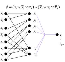
From the discussion earlier, it becomes obvious that SIMP is difficult. In the following, we will prove that SIMP is inapproximable with a non-constant ratio for all , with a gap-introducing reduction from an NP-complete problem 3-SAT to SIMP, where is the number of nodes in an SIG.
Given an expression in CNF, in which each clause has three variables, 3-SAT is to decide whether is satisfiable. The reduction includes two parts: 1) If is satisfiable, its transformed SIMP instance has optimal total adoption larger than . 2) If is unsatisfiable, its transformed SIMP instance has optimal total adoption less than . (Refer Lemma 1 for actual and .) Then inapproximability obtained by this gap-introducing induction is . Note that an -approximation algorithm is able to solve 3-SAT because it always returns a solution larger than for satisfiable and a solution smaller than for unsatisfiable , implying such approximation algorithm must not exist. Also note that the theoretical result only shows that for any algorithm, there exists a problem instance of SIMP (i.e., a pair of an SIG graph and a seed number ) that the algorithm can not obtain a solution better than times the optimal solution. It does not imply that an algorithm always performs badly in every SIMP instance.
Lemma 1
For a positive integer , there is a
gap-introducing reduction from 3-SAT to SIMP, which transforms an -variables expression to an SIMP instance with the SIG as and the as such that
if is satisfiable, , and
if is not satisfiable, ,
where is the optimal solution of this instance, is the number of Boolean variables, and is the number
of clauses.
Hence there is no approximation
algorithm for SIMP unless P NP.
Proof 4.1.
Given a positive integer , for an instance of 3-SAT with Boolean variables and clauses , we construct an SIG with three node sets X, Y and Z as follows. 1) Each Boolean variable corresponds to two nodes , in X and one node in Y. 2) Each clause corresponds to one node in Y. 3) Z has nodes. (Thus, has nodes.) 4) For each in Y, we add direct edges and . 5) For each in Y, we add direct edges , and , where , , are the nodes in X corresponding to the three literals in . 6) We add a hyperedge from all for every . The probability of every edge is set to 1. An example is illustrated in Figure 7.
We first prove that is satisfiable if and only if has a
seed set S with seeds and the total adoption of S contains Y. If is satisfiable, there exists a truth assignment on Boolean variables satisfying all clauses of . Let , and S then has nodes and the total adoption of S contains Y. On the other hand, if is not satisfiable, apparently there
exists no seed set S with exactly one of or selected for every such that the total adoption of S contains Y. For other cases, 1) all seeds are placed in X, but there exists at least one with both and
selected. In this case, there must exist some such that none
of or are selcted (since the
seed number is ), and thus Y is not covered by
the total adoption of S. 2) A seed is placed in Y. In
this case, the seed can be moved to an adjacent without reducing the total adoption. Nevertheless, as explained above,
there exists no seed set S with all seeds placed in X
such that the total adoption of S contains Y, and
thus the total adoption of any seed set with a seed placed in Y
cannot cover Y, either. With above observations, if is not satisfiable, does not have a seed set S with seeds such that the total adoption of S contains Y. Since the nodes of Z can be activated if and only if the total adoption of
S contains Y if and only if is satisfiable, we have
if is satisfiable, , and
if is not satisfiable, .
The lemma follows.
Theorem 4.2.
For any , there is no approximation algorithm for SIMP, assuming P NP.
Proof 4.3.
For any arbitrary , we set . Then, by Lemma 1, there is no approximation algorithm for SIMP unless P NP. Then . Since is arbitrarily small, thus for any , there is no approximation algorithm for SIMP, assuming P NP. The theorem follows.
With Theorem 4.6, no algorithm can achieve an approximation ratio better than . In Theorem 4.8, we prove that SIG-index is correct, and HAG with SIG-index achieves the best ratio, i.e., it is -approximated to SIMP. Note that the approximation ratio only guarantees the lower bound of total adoption obtained by HAG theoretically. Later in Section 6.3, we empirically show that the total adoption obtained by HAG is comparable to the optimal solution.
Theorem 4.4.
HAG with SIG-index is -approximated, where is the number of nodes in SIG.
Proof 4.5.
First, we prove that SIG-index obtains correctly. Assume that there exists an incorrect , i.e., there exists an hyperedge satisfying the conditions in Definition 6 (i.e., and ) but its probability is not aggregated to in . However, the probability can not be aggregated before since and it must be aggregated no later than since . There is a contradiction.
Proving that HAG with SIG-index is an -approximation algorithm is simple. The upper bound of total adoption for the optimal algorithm is , while the lower bound of the total adoption for HAG is because at least one seed is selected. In other words, designing an approximation algorithm for SIMP is simple, but it is much more difficult to have the hardness result for SIMP, and we have proven that SIMP is inapproximable within for any arbitrarily small .
Theorem 4.6.
For any , there is no approximation algorithm for SIMP, assuming P NP.
Proof 4.7.
For any arbitrary , we set . Then, by Lemma 1, there is no approximation algorithm for SIMP unless P NP. Then . Since is arbitrarily small, thus for any , there is no approximation algorithm for SIMP, assuming P NP. The theorem follows.
Corollary 4.8.
HAG with SIG-index is -approximated, where is the number of nodes in SIG.
Proving that HAG with SIG-index is an -approximation algorithm is simple. The upper bound of total adoption for the optimal algorithm is , while the lower bound of the total adoption for HAG is because at least one seed is selected. Note that SIG-index is only for acceleration and does not change the solution quality.
5 Construction of SIG
To select seeds for SIMP, we need to construct the SIG from purchase logs and the social network. We first create possible hyperedges by scanning the purchase logs. Let be the timestamp of a given purchase . ’s friends purchase and her own purchases that have happened within a given period before are considered as candidate source nodes to generate hyperedges to v.111111The considered periods of item inference and social influence can be different since social influence usually requires a longer time to propagate the messages while the item inference on the e-commerce websites can happen at the same time. The detail setting of time period will be discussed in Section 6.1. For each hyperedge , the main task is then the estimation of its their activation probability . Since is unknown, it is estimated by maximizing the likelihood function based on observations in the purchase logs. Note that learning the activation probability for each hyperedge faces three challenges.
C1. Unknown distribution of . How to properly model is critical.
C2. Unobserved activations. When is activated at time , this event only implies that at least one hyperedge successfully activates before . It remains unknown which or hyperedge(s) actually triggers v, i.e., it may be caused by either the item inference or social influence or both. Therefore, we cannot simply employ the confidence of an association-rule as the corresponding hyperedge probability.
C3. Data Sparsity. The number of activations for a user to buy an item is small, whereas the number of possible hyperedge combinations is large. Moreover, new items emerge every day in e-commerce websites, which incurs the notorious cold-start problem. Hence, a method to deal with the data sparsity issue is necessary to properly model a SIG.
To address these challenges, we exploit a statistical inference approach to identify those hyperedges and learn their weights. In the following, we first propose a model of the edge function (to address the first challenge) and then exploit the smoothed expectation and maximization (EMS) algorithm [20] to address the second and third challenges.
5.1 Modeling of Hyperedge Probability
To overcome the first challenge, one possible way is to model the number of success activations and the number of unsuccessful activations by the binomial distributions. As such, is approximated by the ratio of the number of success activations and the number of total activation trials. However, the binomial distribution function is too complex for computing the maximum likelihood of a vast number of data. To handle big data, previous study reported [13] that the binomial distribution can be approximated by the Poisson distribution when the time duration is sufficiently large. According to the above study, it is assumed that the number of activations of a hyperedge follows the Poisson distribution to handle the social influence and item inference jointly. The expected number of events equals to the intensity parameter . Moreover, we use an inhomogeneous Poisson process defined on the space of hyperedges to ensure that varies with different .
In the following, a hyperedge is of size , if the cardinality of its source set is . We denote the intensity of the number of activation trials of the hyperedge as . Then the successful activations of hyperedge follows another Poisson process where the intensity is denoted by . Therefore, the hyperedge probability can be derived by parameters and , i.e., .
The maximum likelihood estimation can be employed to derive . Nevertheless, cannot be derived as explained in the second challenge. Therefore, we use the expectation maximization (EM) algorithm, which is an extension of maximum likelihood estimation containing latent variables to which is modeled as the latent variable. Based on the observed purchase logs, the E-step first derives the likelihood Q-function of parameter with as the latent variables. In this step, the purchase logs and are given to find the probability function describing that all events on in the logs occur according to , whereas the probability function (i.e., Q-function) explores different possible values on latent variable . Afterward, The M-step maximizes the Q-function and derives the new for E-Step in the next iteration. These two steps are iterated until convergence.
With the employed Poisson distribution and EM algorithm, data sparsity remains an issue. Therefore, we further exploit a variant of EM algorithm, called EMS algorithm [20], to alleviate the sparsity problem by estimating the intensity of Poisson process using similar hyperedges. The parameter smoothing after each iteration is called S-Step, which is incorporated in EMS algorithm, in addition to the existing E-Step and M-Step.
5.2 Model Learning by EMS Algorithm
Let and denote the true probability and estimated probabilities for hyperedge in the EMS algorithm, respectively, where . Let and denote the number of activations of source set in the purchase logs and the number of successful activations on hyperedge , respectively. The EM algorithm is exploited to find the maximum likelihood of , while is the latent variable because cannot be observed (i.e., only can be observed). Therefore, E-Step derives the likelihood function for (i.e., the Q-function) as follows,
| (1) |
where is the hyperedge probability derived in the previous iteration, Note that and are given parameters in iteration , whereas is a variable in the Q-function, and is a random variable governed by the distribution . Since is correlated to and , we derive the likelihood as follows.
It is assumed that is independent with , and can be derived as follows:
Since only the first term contains the hidden , only this term varies in different iterations of the EMS algorithm, because in the second term always can be derived by finding the maximum likelihood as follows. Let denote the probability that the source set exactly tries to activate the destination node times, i.e., . The log-likelihood of is
We acquire the maximum likelihood by finding the derivative with regard to :
| (2) |
Thus, the maximum log-likelihood estimation of , representing that the expected activation times (i.e., is . Let denote the action log set, where each log represents that is activated at time . is calculated by scanning and find the times that all the nodes in are activated.
Afterward, we focus on the first term of . Let denote the probability that the hyperedge exactly activates the destination node times. In E-step, we first find the expectation for as follows.
Since and , the log-likelihood of the first term is further simplified as
Afterward, M-step maximizes the Q-function by finding the derivative with regard to :
Therefore, the maximum likelihood estimator is , is , and .
The problem remaining is to take expectation of the latent variables in E-step. Let be the conditional probability that is activated by the source set of at given is activated at , and let denote the set of candidate hyperedges containing every possible with its source set activated at time , i.e., . It’s easy to show that given the estimation of the probability of hyperedges, , since is the probability for to be activated by any hyperedge at time . The expectation of is , i.e., the sum of expectation of each successful activation of from hyperedge , and contains all size hyperedges.
To address the data sparsity problem, we leverage information from similar hyperedges (described later). Therefore, our framework includes an additional step to smooth the results of M-Step. Kernel smoothing is employed in S-Step.
In summary, we have the following steps:
E-Step:
M-Step:
| Dataset | Douban | Gowalla | Epinions | ||||||
|---|---|---|---|---|---|---|---|---|---|
| Precision | Recall | F1-Score | Precision | Recall | F1-Score | Precision | Recall | F1-Score | |
| GT | 0.420916 | 0.683275 | 0.520927 | 0.124253 | 0.435963 | 0.171214 | 0.142565 | 0.403301 | 0.189999 |
| IC | 0.448542 | 0.838615 | 0.584473 | 0.217694 | 0.579401 | 0.323537 | 0.172924 | 0.799560 | 0.247951 |
| SIG | 0.869348 | 0.614971 | 0.761101 | 0.553444 | 0.746408 | 0.646652 | 0.510118 | 0.775194 | 0.594529 |
S-Step: To address the data sparsity problem, we leverage information from similar hyperedges (described later). Therefore, in addition to E-Step and M-Step, EMS includes S-Step, which smooths the results of M-Step. Kernel smoothing is employed in S-Step as follows:
where is a kernel function with bandwidth , and is the mapping function of hyperedges, i.e., maps a hyperedge to a vector. The details of dimension reduction for calculating to efficiently map hyperedges into Euclidean space are shown in the next subsection. If the hyperedges and are similar, the distance of the vectors and is small. Moreover, a kernel function is a positive function symmetric at zero which decreases when increases, and the bandwidth controls the extent of auxiliary information taken from similar hyperedges.121212A symmetric Gaussian kernel function is often used [12]. Intuitively, kernel smoothing can identify the correlation of with and with for nearby and and similar and .
5.3 Dimension Reduction
To facilitate the computation of smoothing function in EMS algorithm, we exploit a dimension reduction technique [24, 27] to map a graph into Euclidean space as a set of vectors. Specifically, given users, let denote the projection matrix, where is the -th row of and is the projection of vertex . We derive as follows:
where is a diagonal matrix, is the identity matrix, and is the Laplacian matrix of distance matrix . This optimization problem attempts to preserve the distance between nodes. However, the constraint restricts that only columns of can be non-zero vector. Therefore, the objective function reduces the dimension of from to while maintaining the local structure as much as possible.
Suppose we solve this generalized eigenproblem for first solutions and the -th component of -th eigenvector is denoted as . The projection of -th node has a -dimensional representation . In our paper, we employ one of the most widely used nonlinear dimension reduction technique, ISOMAP [24] only. The distance matrix , where ( is the identity matrix and is the vector of all ones) and is distance between two nodes in the graph. For our SIG, we first project the users whose graph is , and then the items whose graph is set to be the complete graph. Other method sharing the above optimization formulation can be used as a substitute without much effort.
By employing the above graph embedding approaches, we project the graph into Euclidean space while preserving the distance between the nodes locally. Therefore, the customers who are socially near and the similar commodity items can be extracted efficiently. Therefore, after the dimension reduction procedure, each node has a -dimensional representation. Therefore, each hyperedge of size comprising of source nodes and destination node can be mapped to a vector on the space .
6 Evaluations
We conduct comprehensive experiments to evaluate the proposed SIG model, learning framework and seed selection algorithms. In Section 6.1, we discuss the data preparation for our evaluation. In Section 6.2, we compare the predictive power of the SIG model against two baseline models: i) independent cascade (IC) model learned by implementing [17] and ii) the generalized threshold (GT) model learned by [10].131313http://people.cs.ubc.ca/~welu/downloads.html In addition, we evaluate the learning framework based on the proposed EM and EMS algorithms. Next, in Section 6.3, we evaluate the proposed HAG algorithm for SIMP in comparison to a number of baseline strategies, including random, single node selection, social, and item approaches. Finally, in Section 6.4, we evaluate alternative approaches for diffusion processing, which is essential and critical for HAG, based on SIG-index, Monte Carlo simulations and sorting enhancement.
6.1 Data Preparation
Here, we conduct comprehensive experiments using three real datasets to evaluate the proposed ideas and algorithms. The first dataset comes from Douban [1], a social networking website allowing users to share music and books with friends. Dataset Douban contains users and friendship links, together with (user, music) and (user, bookmark) pairs, representing the music noted and the bookmarks noted by each user, respectively. We treat those (user, music) and (user, bookmark) pairs as purchase actions. In addition to Douban, we adopt two public datasets, i.e., Gowalla and Epinions. Dataset Gowalla contains users, links, and check-ins [7]. Dataset Epinions contains users, links, categories of items, and ratings with timestamp [21]. Notice that we do not have data directly reflecting item inferences in online stores, so we use the purchase logs for learning and evaluations. The experiments are implemented in an HP DL580 server with 4 Intel Xeon E7-4870 2.4 GHz CPUs and 1 TB RAM.
We split all three datasets into 5-fold, choose one subsample as training data, and test the models on the remaining subsamples. Specifically, we ignore the cases when the user and her friends did not buy anything. Finally, to evaluate the effectiveness of the proposed SIG model (and the learning approaches), we obtain the purchase actions in the following cases as the ground truth: 1) item inference - a user buys some items within a short period of time; and 2) a user buys an item after at least one of her friends bought the item. The considered periods of item inference and social influence are set differently according to [14] and [28], respectively. It is worth noting that only the hyperedges with the probability larger than a threshold parameter are considered. We empirically tune to obtain the default setting based on optimal F1-Score. Similarly, the threshold parameter for the GT model is obtained empirically. The reported precision, recall, and F1 are the average of these tests. Since both SIGs and the independent cascade model require successive data, we split the datasets into continuous subsamples.
6.2 Model Evaluation
Tables 1 present the precision, recall, and F1 of SIG, IC and GT on Douban, Gowalla, and Epinions. All three models predict most accurately on Douban due to the large sample size. The SIG model significantly outperforms the other two models on all three datasets, because it takes into account both effects of social influence and item inference, while the baseline models only consider the social influence. The difference of F1 score between SIG and baselines is more significant on Douban, because it contains more items. Thus, item influence plays a more important role. Also, when the user size increases, SIG is able to extract more social influence information leading to better performance than the baselines. The offline training time is 1.68, 1.28, and 4.05 hours on Epinions, Gowalla, Douban, respectively.
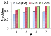
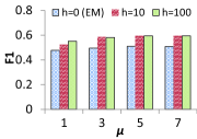
To evaluate the approaches adopted to learn the activation probabilities of hyperedges for construction of SIG, Fig. 8 compares the prevision and F1 of EMS and EM algorithms on Epinions (results on other datasets are consistent and thus not shown due to space limitation). Note that EM is a special case of EMS (with the smoothing parameter , i.e., no similar hyperedge used for smoothing). EMS outperforms EM on both precision and F1-score in all settings of (the maximum size of hyperedges) and tested. Moreover, the precision and F1-score both increases with as a larger overcomes data sparsity significantly. As increases, more combinations of social influence and item inference can be captured. Therefore, the experiments show that a higher improves F1-score without degrades the precision. It manifests that the learned hyperedges are effective for predicting triggered purchases.
6.3 Algorithm Effectiveness and Efficiency
We evaluate HAG proposed for SIMP, by selecting top 10 items as the marketing items to measure their total adoption, in comparison with a number of baselines: 1) Random approach (RAN). It randomly selects nodes as seeds. Note that the reported values are the average of 50 random seed sets. 2) Single node selection approach (SNS). It selects a node with the largest increment of the total adoption in each iteration, until seeds are selected, which is widely employed in conventional seed selection problem [5, 6, 16]. 3) Social approach (SOC). It only considers the social influence in selecting the seeds. The hyperedges with nodes from different products are eliminated in the seed selection process, but they are restored for calculation of the final total adoption. 4) Item approach (IOC). The seed set is the same as HAG, but the prediction is based on item inference only. For each seed set selected by the above approaches, the diffusion process is simulated 300 times. We report the average in-degree of nodes learned from the three datasets in the following: Douban is 39.56; Gowalla is 9.90; Epinions is 14.04. In this section, we evaluate HAG by varying the number of seeds (i.e., ) using two metrics: 1) total adoption, and 2) running time.
To understand the effectiveness, we first compared all those approaches with the optimal solution (denoted as OPT) in a small subgraph sampled, Sample, from the SIG of Douban with 50 nodes and 58 hyperedges. Figures 9 (a) displays the total adoption obtained by different approaches. As shown, HAG performs much better than the baselines and achieves comparable total adoption with OPT (the difference decreases with increased k). Note that OPT is not scalable as shown in Figures 9 (b) since it needs to examine all combination with nodes. Also, OPT takes more than 1 day for selecting 6 seeds in Sample. Thus, for the rest of experiments, we exclude OPT.
Figures 10 (a)-(c) compare the total adoptions of different approaches in the SIG learnt from real networks. They all grow as increases, since a larger increases the chance for seeds to influence others to adopt items. Figure 10 (a)-(c) manifest that HAG outperforms all the other baselines for any in SIG model. Among them, SOC fails to find good solutions since item inference is not examined during seed selection. IOC performs poorly without considering social influence. SNS only includes one seed at a time without considering the combination of nodes that may activate many other nodes via hyperedges.
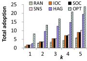
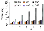

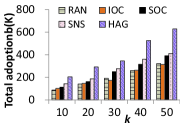
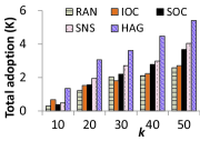
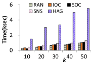
Figure 10 (d) reports the running time of those approaches. Note that the trends upon Gowalla and Epinions are similar with Douban. Thus we only report the running time of Douban due to the space constraint. Taking the source combinations into account, HAG examines source combinations of hyperedges in and obtains a better solution by spending more time since the number of hyperedges is often much higher than the number of nodes.141414To further reduce the running time, we eliminate the source combinations with little gain in previous iterations.
6.4 Online Diffusion Processing
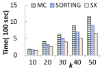
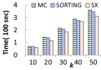
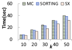
Diffusion processing is an essential operation in HAG. We evaluate the efficiency of diffusion processing based on SIG-index (denoted as SX), in terms of the running time, in comparison with that based on the original Monte Carlo simulation (denoted as MC) and the sorting enhancement (denoted as SORTING), which accesses the hyperedges in descending order of their weights. Figure 11 plots the running time of SX, SORTING, and MC under various using the Douban, Gowalla, and Epinions. For each , the average running times of 50 randomly selected seed sets for SX, SORTING, and MC, are reported. The diffusion process is simulated 300 times for each seed set. As Figure 11 depicts, the running time for all the three approaches grows as increases, because a larger number of seeds tends to increas the chance for other nodes to be activated. Thus, it needs more time to diffuse. Notice that SX takes much less time than SORTING and MC, because SX avoids accessing hyperedges with no source nodes newly activated while calculating the activation probability. Moreover, the SIG-index is updated dynamically according to the activated nodes in diffusion process. Also note that the improvement by MC over SORTING in Douban is more significant than that in Gowalla and Epinions, because the average in-degree of nodes is much larger in Douban. Thus, activating a destination at an early stage can effectively avoid processing many hyperedges later.
7 Conclusion
In this paper, we argue that existing techniques for item inference recommendation and seed selection need to jointly take social influence and item inference into consideration. We propose Social Item Graph (SIG) for capturing purchase actions and predicting potential purchase actions. We propose an effective machine learning approach to construct a SIG from purchase action logs and learn hyperedge weights. We also develop efficient algorithms to solve the new and challenging Social Item Maximization Problem (SIMP) that effectively select seeds for marketing. Experimental results demonstrate the superiority of the SIG model over existing models and the effectiveness and efficiency of the proposed algorithms for processing SIMP. We also plan to further accelerate the diffusion process by indexing additional information on SIG-index.
References
- [1] The Douban dataset download. http://arbor.ee.ntu.edu.tw/~hhshuai/Douban.tar.bz2.
- [2] R. Agrawal, T. Imielinski, and A. N. Swami. Mining association rules between sets of items in large databases. In SIGMOD, 1993.
- [3] R. M. Bond, C. J. Fariss, J. J. Jones, A. D. Kramer, C. Marlow, J. E. Settle, and J. H. Fowler. A 61-million-person experiment in social influence and political mobilization. Nature, 2012.
- [4] S. Bourigault, S. Lamprier, and P. Gallinari. Representation learning for information diffusion through social networks: an embedded cascade model. In WSDM, 2016.
- [5] S. Chen, J. Fan, G. Li, J. Feng, K. Tan, and J. Tang. Online topic-aware influence maximization. In VLDB, 2015.
- [6] W. Chen, C. Wang, and Y. Wang. Scalable influence maximization for prevalent viral marketing in large-scale social networks. In KDD, 2010.
- [7] E. Cho, S. A. Myers, and J. Leskovec. Friendship and mobility: user movement in location-based social networks. In KDD, 2011.
- [8] P. Domingos and M. Richardson. Mining the network value of customers. In KDD, 2001.
- [9] A. Goyal, F. Bonchi, and L. V. S. Lakshmanan. Learning influence probabilities in social networks. In WSDM, 2010.
- [10] A. Goyal, W. Lu, and L. V. S. Lakshmanan. SIMPATH: An efficient algorithm for influence maximization under the linear threshold model. In ICDM, 2011.
- [11] J. Han, M. Kamber, and J. Pei. Data Mining: Concepts and Techniques. Morgan Kaufmann, 3rd Edition, 2011.
- [12] N. L. Hjort and M. C. Jones. Locally parametric nonparametric density estimation. In The Annals of Statistics, 1996.
- [13] R. V. Hogg and E. A. Tanis. Probability and statistical inference. Prentice Hall, 7th Edition, 2005.
- [14] R. Jones and K. Klinkner. Beyond the session timeout: automatic hierarchical segmentation of search topics in query logs. In CIKM, 2008.
- [15] R. J. B. Jr. Efficiently mining long patterns from databases. In SIGMOD, 1998.
- [16] D. Kempe, J. M. Kleinberg, and É. Tardos. Maximizing the spread of influence through a social network. In KDD, 2003.
- [17] H. Li, T. Cao, and Z. Li. Learning the information diffusion probabilities by using variance regularized em algorithm. In ASONAM, 2014.
- [18] J. Nail. The consumer advertising backlash, 2004. Forrester Research and Intelliseek Market Research Report.
- [19] N. Pasquier, Y. Bastide, R. Taouil, and L. Lakhal. Discovering frequent closed itemsets for association rules. In ICDT, 1999.
- [20] B. W. Silverman, M. C. Jones, J. D. Wilson, and D. W. Nychka. A smoothed em approach to indirect estimation problems, with particular, reference to stereology and emission tomography. Journal of the Royal Statistical Society. Series B (Methodological), 1990.
- [21] J. Tang, H. Gao, H. Liu, and A. D. Sarma. etrust: Understanding trust evolution in an online world. In KDD, 2012.
- [22] J. Tang, S. Wu, and J. Sun. Confluence: conformity influence in large social networks. In KDD, 2013.
- [23] Y. Tang, X. Xiao, and Y. Shi. Influence maximization: near-optimal time complexity meets practical efficiency. In SIGMOD, 2014.
- [24] J. B. Tenenbaum, V. d. Silva, and J. C. Langford. A global geometric framework for nonlinear dimensionality reduction. Science, 2000.
- [25] H. Vahabi, I. K. F. Gullo, and M. Halkidi. Difrec: A social-diffusion-aware recommender system. In CIKM, 2015.
- [26] Z. Wen and C.-Y. Lin. On the quality of inferring interests from social neighbors. In KDD, 2010.
- [27] S. Yan, D. Xu, B. Zhang, H.-J. Zhang, Q. Yang, and S. Lin. Graph embedding and extensions: A general framework for dimensionality reduction. IEEE Transactions on Pattern Analysis and Machine Intelligence, 2007.
- [28] J. Yang and J. Leskovec. Modeling information diffusion in implicit networks. In ICDM, 2010.