Herschel Hi-GAL imaging of massive young stellar objects

Abstract

We used Herschel Hi-GAL survey data to determine whether massive young stellar objects (MYSOs) are resolved at 70$\mu$m and to study their envelope density distribution. Our analysis of three relatively isolated sources in the $l=30$^∘ and $l=59$^∘ Galactic fields show that the objects are partially resolved at 70$\mu$m. The Herschel Hi-GAL survey data have a high scan velocity which makes unresolved and partially resolved sources appear elongated in the 70$\mu$m images. We analysed the two scan directions separately and examine the intensity profile perpendicular to the scan direction. Spherically symmetric radiative transfer models with a power law density distribution were used to study the circumstellar matter distribution. Single dish sub-mm data were also included to study how different spatial information affects the fitted density distribution. The density distribution which best fits both the 70$\mu$m intensity profile and SED has an average index of $\sim 0.5$. This index is shallower than expected and is probably due to the dust emission from bipolar outflow cavity walls not accounted for in the spherical models. We conclude that 2D axisymmetric models and Herschel images at low scan speeds are needed to better constrain the matter distribution around MYSOs.

1 Introduction

The formation of massive stars presents many challenges due to the competing and interlinked roles of gravity, magnetic fields and radiation. It is becoming clear through numerical simulations that material can continue to accrete on to a luminous, massive forming star via an accretion disc despite the strong radiation pressure on dust (Krumholz et al. 2009; Kuiper et al. 2010). Bipolar outflows appear to be a ubiquitous ingredient in the star formation process driven by magnetic forces (Banerjee & Pudritz 2007) which also helps relieve the extreme radiation pressure (Cunningham et al. 2011).

These competing infall and outflow processes shape the circumstellar matter distribution around massive forming stars. The corollary of this is that a detailed mapping of the circumstellar matter distribution can be used to constrain models of massive star formation. One way to probe the circumstellar matter close to the protostar is to use the emission from the heated dust. This has some advantages over using molecular line emission for which complex chemical and excitation effects have to be taken into account before the total gas density distribution can be recovered. There are also disadvantages with using warm dust emission as it does not convey any kinematic information and becomes optically thick for $\lambda<100$$\mu$m. However, a full understanding of the dust emission also yields the temperature distribution of the material which is an important input back into the molecular line diagnostic process.

Different IR wavelengths will probe regions at different distances from the central accreting source due to the temperature gradients. Typical temperature gradients vary from $T\propto r^{-3/4}$ in the optically thick part to $T\propto r^{-1/2}$ in optically thin regions (eg. Ivezić & Elitzur 1997). Taking the over-simplified approach of the Wien Displacement law to locate where most of the emission arises from, we then see that the size of the emitting region $r\propto\lambda^{4/3}$ or $r\propto\lambda^{2}$ in optically thick and thin regions respectively. In the immediate environment of a protostar we will have optically thick conditions in the dense mid-plane regions whilst the bipolar outflow cavities will be mostly optically thin.

High resolution studies of the warm dust emission around massive forming stars have included the 8-13$\mu$m interferometric studies by de Wit et al. (2007;2010;2011). These 40 milliarcsecond resolution studies probe size scales of about 100 AU for typical distances of nearby massive young stellar objects (MYSOs) which approaches the size of the dust sublimation radius of about 25 AU. The mid-IR visibilities are mostly matched by 2D axisymmetric radiative transfer models where most of the emission arises from the warm dust along cavity walls. A compact element inside the dust sublimation radius such as an accretion disc may be needed to explain the rising 8$\mu$m visibilities.

Since the dusty bipolar cavity walls are directly illuminated by the central star then this is mostly optically thin emission. We would therefore expect the size of the emitting region to scale as $\lambda^{2}$. For single-dish observations then this size scale is getting larger faster than the diffraction-limited resolution is degrading. Hence, for a given diameter telescope it is better to use the longest wavelength possible. For the thermal-IR regime from the ground this is 24.5$\mu$m at the far end of the Q band. Scaling from the 60 milliarcsecond size for W33A at 13$\mu$m (de Wit et al. 2007) this would yield a size of 0.2″ at 24.5$\mu$m which would be partially resolved by the 0.6″ diffraction limit for 8 m telescopes. This is what was found by de Wit et al. (2009) and Wheelwright et al. (2012) who partially resolved a sample of massive YSOs. de Wit et al. (2009) modelled the extended emission with spherical models and concluded that the density distribution needed to be $n\propto r^{-1}$. This was interpreted as requiring some rotational support on these scales as it is shallower than the $n\propto r^{-1.5}$ expected for free-falling material. Wheelwright et al. (2012) again used 2D axisymmetric radiative transfer models to show that the 20$\mu$m emission is also dominated by the warm envelope dust along the cavity walls. This is seen explicitly in some edge-on systems (e.g. De Buizer 2005; 2006).

The recent release of Herschel space telescope data provides the highest resolution images to date at far-IR wavelengths. If we extend the scaling above to the shortest wavelength of Herschel of 70$\mu$m then we would expect a size of the emitting region of about 2″. This is comparable to the 5″ diffraction-limited beam of Herschel at 70$\mu$m. Hence, we expect to recover further spatial information on the somewhat cooler dust located further from the central object, but not so far as to be more influenced by the general molecular core environment and ambient radiation field as is likely at the longer Herschel wavebands.

The most extensive observations of massive forming stars with Herschel comes from the Hi-GAL survey of the Galactic Plane (Molinari et al. 2010a) where most massive young stars are located. Here we examine these data from the first two Science Demonstration Phase fields observed as part of Hi-GAL (Molinari et al. 2010a) to determine whether massive YSOs are indeed extended at 70$\mu$m.

We define massive YSOs as deeply embedded, luminous (L$\,\stackrel{{\scriptstyle\raisebox{-0.60275pt}{$\textstyle>$}}}{{\sim}}\,$3000L_⊙), mid-IR-bright, point sources that are not ionizing their surroundings to form an ultra-compact H II region (UCHII). The lifetime of this phase is about 10⁵ years (Davies et al. 2011; Mottram et al. 20111a). Davies et al. (2011) show that the luminosity function of MYSOs and UCHII regions is consistent with the MYSOs becoming swollen due to high accretion rates as predicted by the models of Hosokawa & Omukai (2009). This means their effective temperatures are too low to ionise their surroundings until either they stop accreting at high rates or grow to greater than about 30M_⊙, when they contract rapidly down to their main sequence radius.

The sample of MYSOs we use comes from the Red MSX Survey (RMS) (Lumsden et al. 2013). Starting from an initial colour selection of mid-IR bright sources (Lumsden et al. 2002) from the MSX satellite point source catalogue (Price et al. 2001) we have followed these up with radio continuum observations to distinguish UCHII regions and dusty planetary nebulae (Urquhart et al. 2009); determined kinematic distances from ¹³CO observations and H I absorption (Urquhart et al. 2008; 2012); and determined luminosities from far-IR fluxes (Mottram et al. 2010; 2011b). All MYSOs discussed in this paper are undetected at 5 GHz at the 1 mJy level.

In this paper we examine the Herschel imaging of the RMS MYSOs in two lots of 2 square degree regions of the Galactic plane. The peculiarities of the Hi-GAL 70$\mu$m point spread function (PSF) are discussed in section 2 and the 70$\mu$m imaging of the RMS MYSOs in these regions is described in section 3. Radiative transfer modelling of the 70$\mu$m emission is presented in section 4 and the results discussed in section 5. Conclusions are drawn in section 6.

2 Hi-GAL 70$\mu$m Point Spread Function

The Hi-GAL survey was carried out in a specially developed parallel mode whereby the PACS and SPIRE instruments simultaneously scan the sky at a fast rate of 60″ per second (Molinari et al. 2010). This causes the nominally circular PACS 70$\mu$m beam with FWHM of 5.3″ to be smeared out in the scan direction with a resultant size of 5.8″ $\times$ 12.1″ (Lutz 2012). A high signal-to-noise representation of the PACS parallel mode 70$\mu$m PSF is shown in figure 1, which shows an image of the asteroid Vesta observed in similar conditions as Hi-GAL data (see Lutz 2012). The first Airy ring can also be seen smeared out along the scan direction (PA=42.5^∘) and a dark spot is seen at one end of the scan direction.

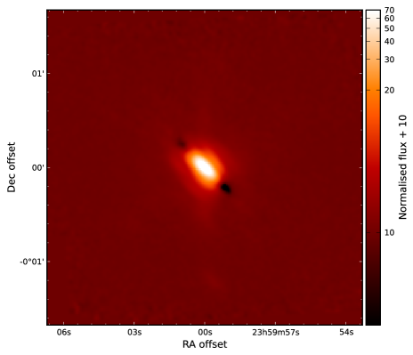
Figure 1: Image of Vesta taken in parallel mode with a scan speed of 60″ per second and array-to-map inclination angle of $\alpha=$ 42.5^∘ showing the details of the point spread function. In order to use a logarithmic stretch, a constant value of 10 was added to the normalised fluxes.

The two Science Demonstration Phase (hereafter SDP) Hi-GAL fields were visually inspected to search for objects that might be suitable PSF objects at 70$\mu$m, i.e. bright, unresolved and isolated. Such objects are rare and we only found two in each of the SDP fields and their details are listed in table 1. These appear to be all AGB or post-AGB stars and they were all located away from the mid-plane consistent with an evolved, intermediate mass population. Such stars are losing mass with dusty winds which makes them suitable for IR PSF stars. However, as de Wit et al. (2009) found these stars can also be extended and so have to be treated with caution when using as PSF objects.

Table 1: Parameters of the PSF objects found within the two Hi-GAL SDP fields at 70$\mu$m.

Name	Nature	RA	Dec	$f_{70\mbox{$\mu$m}}$
		(J2000)		(Jy)
V1362 Aql	Mira	18:48:41.9	$-$02:50:28	66
IRAS 18491$-$0207	PAGB	18:51:46.2	$-$02:04:12	80
IRAS 19374+2359	PAGB	19:39:35.5	$+$24:06:27	29
IRAS 19348+2229	?	19:36:59.8	$+$22:36:08	32

An image of the PSF object V1362 Aql from the l=30^∘ SDP field is shown in figure 2. This is from the so-called naive map constructed from the Hi-GAL data which adds together the two different scan directions referred to as nominal and orthogonal. Unfortunately this results in a complex PSF which is basically a cross-shape. The naive maps we used had not had any astrometric corrections applied, which also resulted in an offset cross-shape. Such a complex PSF makes the search for extended emission very difficult and certainly precludes the use of azimuthally averaged radial profiles as we used for ground-based 24$\mu$m imaging (de Wit et al. 2009; Wheelwright et al. 2012). We decided to analyse images made from the nominal and orthogonal scans separately which maximises the resolution in the minor axis of the elongated PSF.

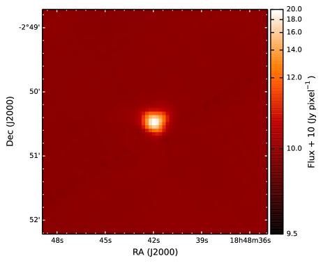
Figure 2: Image of the PSF star V1362 Aql in the naive map of the l=30 region. Note the offset cross shape caused by the addition of the nominal and orthogonal scans each of which has an elongated PSF.

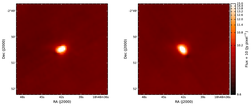
Figure 3: Nominal (left) and orthogonal (right) scan image of the PSF star V1362 Aql. The flux scale is the same for both images.

We compared the Vesta PSF to that of the PSF objects from the SDP field. This was to make sure that they were consistent with each other as the PSF changes because the angle between the scan and the detector axis (hereafter array-to-map angle, $\alpha$) changes with map direction (Lutz 2012). The values of the array-to-map angle used are $\alpha=+42.5$^∘ for the nominal direction, same as Vesta in figure 1, and $\alpha=-42.5$^∘ for the orthogonal direction (Molinari et al. 2010a). Separate scan images of the PSF object V1362 Aql are shown in figure 3. The structure in these images is similar to that in the Vesta image in figure 1. Each Vesta image was rotated so that the major axis was horizontal and the scan direction pointing to the right, and then rebinned to the coarser pixel scale used in Hi-GAL as in figure 4. A vertical slice was then taken along the minor axis, three pixels wide and centred on the peak pixel. Each of the three columns were normalised to the central peak value and then a mean and standard deviation were taken from the three values at each offset position.

The same procedure was applied to the nominal and orthogonal PSF objects after first subtracting a mean background level determined in an annulus surrounding the object, and the intensity profile of the slices compared. The images were rotated so the positive scan legs point in the same direction as the rebinned Vesta image. To ensure the best comparison between objects at the subpixel level, a 2D Gaussian was fitted to the image and the slice was shifted so that the zero offset coincides with the Gaussian peak.

Figure 5 shows that the intensity slices of the rebinned Vesta and the PSF stars V1362 Aql and IRAS 18491-0207 drop to about 1% of the peak or about 14″ from the centre, which is where the uncertainties on the background level of the PSF objects become significant. Hence, since most of the MYSO targets are of similar or brighter flux than these PSF objects, comparing the MYSOs to these PSF objects would introduce more noise especially in the wings. Therefore, we compared our MYSOs to the much higher signal-to-noise image of Vesta from figure 1.

It is also worth noticing that the minor axis of the PSF objects is independent of whether the object was present in one (e.g. IRAS 18491-0207 orthogonal) or both (e.g. IRAS 18491-0207 nominal) scan legs. However, for the purpose of modelling the continuum emission (see Section 4) a Vesta image averaged with its reflection along the major axis was used for sources present in both scan legs. The difference along the minor axis slice is less than 10% between this averaged Vesta slices and the original one.

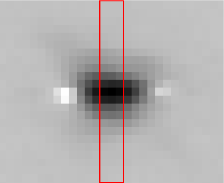
Figure 4: Image of Vesta ($\alpha=42.5$^∘) rotated and rebinned to Hi-GAL resolution showing the slice along the minor axis used in this work (red box). Each pixel has a size of 3.2″ and the image is $29\times 23$ pixels in size.

3 Observations

3.1 70$\mu$m Imaging of RMS MYSOs

There are a total of 12 RMS MYSOs in the $l$=30^∘ SDP field and 7 in the $l$=59^∘ field. We visually inspected each of these and found that only one in the $l$=30^∘ and two in the $l$=59^∘ field were sufficiently isolated from neighbouring sources and/or complex background (e.g. filamentary structures) emission to allow an investigation of their extended emission. The parameters of the these MYSOs are given in table 2. Figure 6 shows the naive 70$\mu$m map of the brightest of the MYSOs, G030.8185+00.2729, and an example MYSO ignored for its complex background and the presence of a nearby object, G030.4117-00.2277. In our sampled objects, between 2 to 4 point sources were detected at 8$\mu$m in the GLIMPSE/IRAC observations within the Herschel 70$\mu$m resolution ($\sim 6$″), but $\gtrsim 50$% of the emission is dominated by the MYSO at 8$\mu$m and totally dominates in MIPS 24$\mu$m images. Therefore, in what follows we will not consider multiplicity as major concern.

Table 2: Parameters of the isolated RMS MYSOs found within the two Hi-GAL SDP fields at 70$\mu$m.

Name	RA	Dec	d	L	$\sqrt{\rm L}$/d b	$f_{70\mbox{$\mu$m}}$	$f_{170\mbox{$\mu$m}}$	$f_{250\mbox{$\mu$m}}$	$f_{350\mbox{$\mu$m}}$	$f_{500\mbox{$\mu$m}}$
			(kpc)	(L⊙)	(L⊙1/2 kpc-1)	(Jy)	(Jy)	(Jy)	(Jy)	(Jy)
G030.8185+00.2729	18:46:36.6	$-$01:45:22	5.7	1.1$\times 10^{4}$	18.4	321	269	131	57.6	22.7
G058.7087+00.6607	19:38:36.8	$+$23:05:43	4.4	4.4$\times 10^{3}$	15.1	30.9	70.5	44.4	23.2	12.2
G059.8329+00.6729	19:40:59.3	$+$24:04:44	4.2	1.9$\times 10^{3}$a	10.4	150	361	150	61.0	25.2

^a Note this object is in a cluster with several other YSOs within about 5″. Its GLIMPSE 8$\mu$m flux is only 20% of the larger MSX beam 8$\mu$m flux and its total luminosity has therefore been reduced by this amount to reflect the fact there may be other luminosity sources in the large beam far-IR measurements of bolometric luminosity (see Mottram et al. 2011).

^b The physical size of a spherical dusty cloud heated to a particular temperature by a central source depends on the square root of the heating source luminosity which determines the spatial scales of the solution to the radiative transfer equation (Ivecić & Elitzur 1997). The angular size is then inversely proportional to the distance. Therefore, it is an indicator of how resolved is a source (see Section 5).

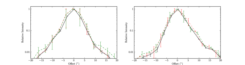
Figure 5: A comparison of the intensity profile of Vesta (solid black line) and PSF stars V1362 Aql (dash-dotted red line) and IRAS 18491$-$0207 (dashed green line) slices in the nominal (left) and orthogonal (right) map directions. Note the agreement within the errors between Vesta and the PSF objects out to about the 1% level.

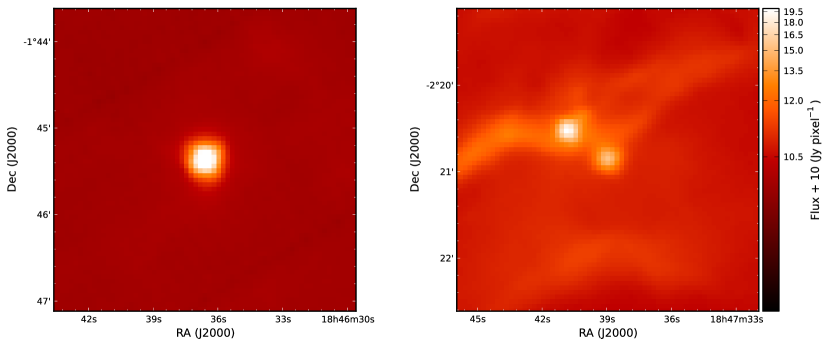
Figure 6: Image of the RMS MYSOs G030.8185+00.2729 (left) and G030.4117-00.2277 (right) from the naive map of the l=30 region. Note the partially resolved nature of G030.8185+00.2729 compared to the PSF star in figure 2 and the background level and morphology compared to G030.4117-00.2277.

Comparing G030.8185+00.2729 in figure 6 to the naive map of the PSF star V1362 Aql in figure 2, clearly shows that the former is more extended compared to the PSF star. Similarly, figure 7 shows the nominal and orthogonal scan images for G030.8185+00.2729 and these clearly show extended emission along the minor axis direction compared to the PSF star in figure  3. Intensity profiles for slices along the minor axis were constructed for each of the MYSOs as described above for the PSF objects. In figures 8 to 10 these slices (square blue points with error bars) are compared with those for Vesta (dashed cyan line). Again the 70$\mu$m emission from the MYSO is clearly more extended in the minor axis direction than the Herschel PSF for all the MYSOs in both scan directions.

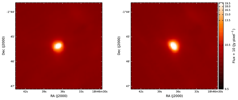
Figure 7: Nominal (left) and orthogonal (right) scan images for the RMS MYSO G030.8185+00.2729. The flux scale is the same for both images.

3.2 Sub-mm Radial Profiles

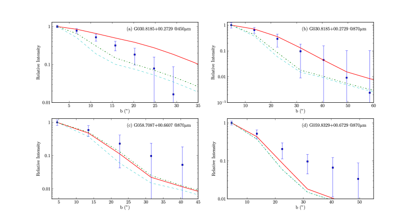
Figure 11: Azimuthally averaged radial profiles of sub-mm observations for each source (blue squares). The radial profiles from the best fitted models using the 70$\mu$m intensity profile and SED for nominal (solid red line) and orthogonal (dash-dotted green line) directions are also shown. (a) and (b) show G030.8185+00.2729 radial profiles for 450 and 870$\mu$m, respectively. (c) and (d) show the 870µm radial profile of G058.7087+00.6607 and G059.8329+00.6729, respectively. The dashed cyan line corresponds to the PSF. The impact parameter $b$ corresponds to the angular distance to the peak of the emission in the plane of the sky.

Although Herschel images of the same fields at 160, 250, 350 and 500$\mu$m are available, we limited the use of these images only for the SED. However, ground-based sub-mm observations are available which are at higher resolution. Azimuthally averaged radial profiles at 870$\mu$m were obtained from ATLASGAL images (Contreras et al. 2013) and at 450$\mu$m from the SCUBA Legacy Catalogues (Di Francesco et al. 2008) and are shown in figure 11. Annulii of 1.5 times the pixel size (6″ at 870$\mu$m and 3″ at 450$\mu$m) were chosen to compute the average flux in each bin of angular distance from the peak. The errors in each bin were estimated by the standard deviation of the fluxes in each annulus.

4 Results

To interpret the extended emission that we see at 70$\mu$m we have adapted the modelling procedure used by de Wit et al. (2009). We used the same grid of spherical radiative transfer models for MYSOs that was calculated by de Wit et al. (2009) using the DUSTY code (Ivezić & Elitzur 1997). The grid of 120 000 models spans a range in density law exponent $p$ where $n(r)\propto r^{-p}$ with $p$ varying from 0 to 2 in steps of 0.5, A_V from 5 to 200 in steps of 5, and the ratio of outer radius to sublimation radius, $Y\equiv R_{outer}/R_{sub}$, varying from 10 to 5000. For this study other model grid parameters were kept constant. These include the stellar effective temperature that was kept at 25 000 K corresponding to a B0 V star as the IR emission is insensitive to this parameter. For the dust model we used the ’ISM’ model as described in de Wit et al. (2009) that consists of Draine & Lee (1984) graphite and silicate with an MRN size distribution (Mathis et al. 1977). This has a sub-mm emissivity law with a slope of $\beta=2$. The dust sublimation temperature was kept constant at 1500 K.

Each model was scaled to the appropriate luminosity and distance for the MYSOs in table 2. A circular image of the emergent 70$\mu$m emission from the spherical model was generated and then convolved with the Vesta PSF rebinned for the Hi-GAL pixel scale. As before, an intensity profile slice was generated from an average of the three rows across the minor axis of the PSF direction normalised to the peak pixel. These model slices were then compared to the observed ones, both in the nominal and orthogonal scan directions.

Simultaneously with fitting the intensity profile slice we also fitted the spectral energy distributions (SEDs). The luminosity used to scale the models comes from fitting the SED. The data points in the SEDs in figures 8 to 10 are from 2MASS (Skrutskie et al. 2006), GLIMPSE (Churchwell et al. 2009), MSX (Price et al. 2001), Herschel (this work), sub-millimetre (Di Francesco et al. 2008; Contreras et al. 2013) and millimetre observations (Beuther et al. 2002; Beltrán et al. 2006). Errors of 10% were adopted for all the SED data points to account for uncertainties in the absolute calibration across different datasets. During the fitting procedure reduced-$\chi^{2}$ (hereafter $\chi^{2}$) values were calculated for both the fits to the intensity slice and SED, where the degrees of freedom were the number of fitted points minus one. These are each placed in order of increasing $\chi^{2}$ and the model that is top of the combined order is considered to be the best fitting model (e.g. de Wit 2009).

The best combined fits to the 70$\mu$m intensity profile and SED for each direction are shown in figures 8 to 10 whilst the parameters are listed in table 3. In what follows, the results are not referred to any particular scan direction unless otherwise stated. Reasonable combined fits to the intensity profile of most of the objects are obtained with the models, with $\chi^{2}$ near 1 for the 70$\mu$m profile. The SED fit shows that fluxes at $\lambda<3$$\mu$m are always underestimated. This is common for spherical models as they do not account for near-IR light being scattered and escaping from the bipolar outflow cavities (de Wit et al. 2010). The average power law index of the best fitting models is $p=0.5$.

Figure 11 show the profiles at 450 and 870$\mu$m as seen in the combined fit of the SED and 70$\mu$m intensity profile. Sub-mm radial profiles were also used instead of the 70$\mu$m slices to analyse the effects of the spatial information from different wavelengths on the density distribution fit. These profiles constrain the density distribution of the cool outer regions. The combined 850/450$\mu$m profile and SED best fits have an average exponent $p=0.5$, which is consistent with the combined 70$\mu$m profile and SED fit.

Finally, fits to each individual observation were also calculated. The results show that the best fits to radial profiles have exponents between 1 and 2, whilst the fits to SEDs have exponents between 0 and 0.5. In addition, the exponent of the best fitted models to the radial profiles is independent of A_V and the size of the cloud.

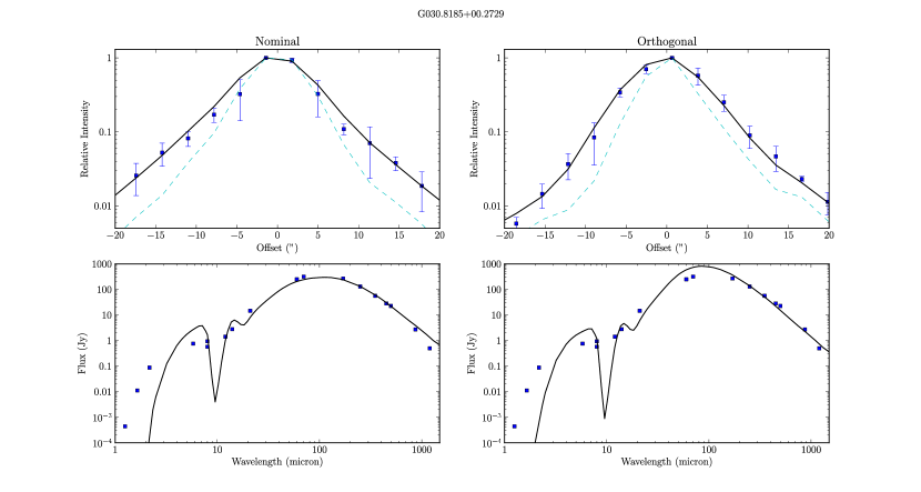
Figure 8: The combined best fit model (solid black) in terms of the 70$\mu$m scan profile (top) and SED (bottom) compared to the data (blue squares) for G030.8185+00.2729. The left hand panels are for the scan in the nominal direction whilst the right hand panel is for the scan in the orthogonal direction. The Vesta PSF scan is shown in the top panel (dashed cyan) to illustrate the extended nature of the MYSO emission. An error of 10% of the total observed fluxes was considered in the observed SED.

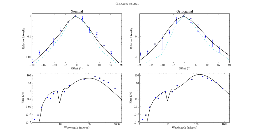
Figure 9: As in figure 8 but for G058.7087+00.6607.

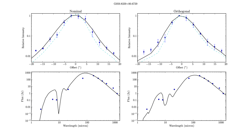
Figure 10: As in figure 8 but for G059.8329+00.6729.

5 Discussion

The average power law index is shallower than the $p\sim 1$ exponent in the sample of de Wit et al. (2009) who fitted 24.5$\mu$m intensity profiles and SED. In addition, our averages do not agree in general with other works which have found that the values of the power law index vary between $1$ and $2$ by combining SED and sub-mm observations (e.g. Mueller et al. 2002). Nevertheless, in the particular case of G030.8185+00.2729, Williams et al. (2005) obtained an exponent of $0.5$ by using the SED and 850$\mu$m radial profile, which agrees with our results. The results of Williams et al. (2005) where obtained by including in the SED points with $\lambda\geqslant 12$$\mu$m whilst Mueller et al. (2002) included points with $\lambda\geqslant 30$$\mu$m. We experimented with also only fitting data with $\lambda\geqslant 30$$\mu$mand found that in general values of exponents are 0.5 lower than using the whole SED, and therefore the exponents are still between 0 and 1. We obviously do not expect to match the average results of Mueller et al. and de Wit et al. since our sample has only 3 objects.

The power law indexes for the slice only and 870$\mu$m only cases vary between $1.5$ and $2$, whilst in the 450$\mu$m only cases its value is $p=1$. These values are consistent with those obtained by Beuther et al. (2002), who found an average value of $p=1.6$, even though they derived their values from a power law fitted to the radial profiles instead of doing the radiative transfer. Of course, these models do not fit the SED well.

On the other hand, the power law indexes for the fits to the SED only vary between $0$ and $0.5$. This is similar to previous studies that use a dust emissivity law with a slope of $\beta=2$ (e.g. Chini et al. 1986). As discussed by Hoare et al. (1991), a shallower dust emissivity law allows fits with a steeper density distribution. In fact, inspection of the SED fits at $\lambda>100$$\mu$m in figure 9 appears to show that the $\lambda^{-2}$ emissivity law used in the modelling is slightly too steep. Moreover, a study of the dust emissivity law in these two regions by Paradis et al. (2010) shows that the emissivity slope should be $\sim 1.5$ in $l=30$^∘ and $\sim 1$ in $l=59$^∘ for a dust temperature of 30 K. Our higher value of the slope would also explain the large values of A_V, for steeper emissivity laws need more dust mass to match the dust emission in the far-IR/submm.

The values of A_V range between 95 and 200 for the combined SED and slice fit, but most of the sources have an A_V of 200. This is consistent with them being massive, young and embedded objects in their parental clouds. However, de Wit et al. (2009) found lower values than ours. In the particular case of G030.8185+00.2729, Williams et al. (2005) found a value $\sim 4$ times larger than ours, and using the method of Mueller et al. (2002) we obtain similar values of A_V as those obtained by considering all the points in the SED. Either way, all these results point towards values of A_V greater than 90 magnitudes, and the inclusion of points at smaller wavelengths does not determine the value of A_V though it helps to constrain it. The value of A_V seems to be determined by the amount of dust necessary to reproduce the far-IR/sub-mm dust emission given its emissivity law.

Table 3: Best fit model parameters for the fits to the 70$\mu$m intensity slice and the 450$\mu$m and 870$\mu$m radial profiles.

Name	Scan	Fit	$p$	AV	$Y^{a}$	$\chi^{2}_{SED}$	$\chi^{2}_{70\mbox{$\mu$m}}$	$\chi^{2}_{450\mbox{$\mu$m}}$	$\chi^{2}_{870\mbox{$\mu$m}}$
G030.8185+00.2729	nominal	SED + 70$\mu$m	1.0	200	5000	109	1.4	4.7	0.23
		SED + 450$\mu$m	0.5	170	2000	40	3.2	0.4	1.48
		SED + 870$\mu$m	0.5	120	5000	73	3.6	4.1	0.04
	orthogonal	SED + 70$\mu$m	0.5	200	1000	77	0.7	1.9	2.17
		SED + 450$\mu$m	0.5	170	2000	40	1.6	0.4	1.48
		SED + 870$\mu$m	0.5	120	5000	73	13.6	4.1	0.04
G058.7087+00.6607	nominal	SED + 70$\mu$m	1.0	120	5000	132	0.6	…	0.48
		SED + 870$\mu$m	0.5	150	5000	62	3.2	…	0.25
	orthogonal	SED + 70$\mu$m	0.0	95	5000	45	2.6	…	0.35
		SED + 870$\mu$m	0.5	150	5000	62	2.8	…	0.25
G059.8329+00.6729	nominal	SED + 70$\mu$m	0.5	200	1000	4800	4.8	…	1.42
		SED + 870$\mu$m	0.5	200	5000	101	6.2	…	0.57
	orthogonal	SED + 70$\mu$m	0.0	200	2000	403	1.5	…	1.88
		SED + 870$\mu$m	0.5	200	5000	101	2.0	…	0.57

Notes: The values of $\chi^{2}$ correspond to the reduced $\chi^{2}$.

^a $Y\equiv R_{outer}/R_{sub}$ with $R_{outer}$ the outer radius and $R_{sub}$ the sublimation radius of the envelope

Table 2 shows the values of the $\sqrt{\rm L}$/d ratio, which has previously found to be a good indicator of how resolved these objects are (e.g. Wheelwright et al. 2011). This ratio is proportional to the angular size of the inner rim of the spherical envelope (Ivecić & Elitzur 1997) and, as is shown in table 3, the envelopes have sizes a few thousands times the sublimation radius ($\sim 25$ au for $\rm L=10^{4}$L_⊙), and should therefore be resolved at longer wavelengths. Figures 8 to 10 show the degree to which the objects are resolved at 70$\mu$m agrees with this.

To explore whether this extends to the other 16 MYSOs with more complex background/neighbouring sources, we repeat the procedures used in the previous sections to obtain slices from the other sources in the Hi-GAL fields and from two models with similar physical properties as those obtained by the radiative transfer results, and then fitted 1D Gaussian to measure the FWHM of these slices to see how resolved the sources are. Figure 12 shows the relation between the FWHM and the $\sqrt{\rm L}/\rm d$ ratio. All observed sources are consistent with the models with some of them more extended due to the complex background.

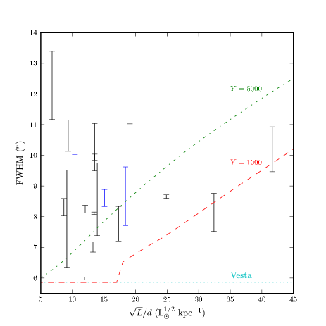
Figure 12: Relation between $\sqrt{\rm L}/\rm d$ and FWHM of a 1D Gaussian fitted to the 70$\mu$m slices from MYSOs in the $l=30$^∘ and $l=59$^∘ fields and models. The bar ranges are defined by the FWHM of the fit to the nominal and orthogonal directions, and the blue bars correspond to our sample. The predicted relation from two models with $p=0.5$ and A${}_{\rm V}=200$ is shown in red dashed line for $Y=1000$ and in greed dot-dashed line for $Y=5000$. Model images were convolved with the nominal Vesta PSF and a mean error of 1.2″ is estimated for the Gaussian fit. The horizontal cyan dotted line represents the FWHM of the Vesta nominal slice.

6 Conclusions

We have presented 70$\mu$m observations made with the Herschel PACS instrument towards two regions of the Galactic plane and identified three relatively isolated MYSOs. The peculiarities of the Hi-GAL survey PSF and its effects on the MYSOs observations were analysed. The sources in our sample are all partially resolved at 70$\mu$m.

Using spherical radiative transfer models to simultaneously fit the 70$\mu$m profile and SED, we find we need a density law exponent of around 0.5. This is shallower than we previously found from fitting partially resolved 24.5$\mu$m ground-based imaging, though both observations give an exponent between 0 and 1. It is also shallower than expected for infalling material ($p=1.5$). This could be due to rotational support, but since the emitting region is well outside of the expected disk/centrifugal radius (less than a few thousands AU, e.g. Zhang 2005) this is unlikely. It is more likely due to warm dust along the outflow cavity walls as seen in the mid-IR. We will investigate this further using 2D axisymmetric models. Intrinsic asymmetry could explain why we do not always get the same results on the same object from the nominal and orthogonal scan directions.

Finally, the images at 70$\mu$m were smeared along the scan direction due to the scan speed. Moreover, the lack of PSF stars in the fields does not allow a characterisation of the PSF specific for these observations. Therefore, slow scan data, with a better behaved PSF, will be better to map and constrain the matter distribution of MYSOs. In particular, if the dust emission at 70$\mu$m comes from a non-spherical structure like bipolar cavity walls, data at 70$\mu$m can provide useful insights for 2D models.

References

Banerjee, R. & Pudritz, R. E. 2007, ApJ, 660, 479

Beltrán, M. T., Brand, J., Cesaroni, R., Fontani, F., Pezzuto, S., Testi, L., & Molinari, S. 2006, A&A, 447, 221

Beuther, H., Schilke, P., Menten, K. M., Motte, F.; Sridharan, T. K.; Wyrowski, F. 2002, ApJ, 566, 945

Chini, R., Kruegel, E., & Kreysa, E. 1986, A&A, 167, 315

Churchwell, E., et al. 2009, PASP, 121, 213

Contreras, Y., Schuller, F., Urquhart, J. S., et al. 2013, A&A, 549, A45

Cunningham, A. J., Klein, R. I., Krumholz, M. R., McKee, C. F. 2011, ApJ, 740, 107

Davies, B. et al. 2011, MNRAS, 416, 972

De Buizer, J. M., 2006, ApJ, 642, L57

De Buizer, J. M., 2007, ApJ, 654, L147

de Wit, W. J., Hoare, M. G., Oudmaijer, R. D., & Mottram, J. C. 2007, ApJ, 671, L169

de Wit, W. J., Hoare, M. G., Fujiyoshi, T., et al. 2009, A&A, 494, 157

de Wit, W. J., Hoare, M. G., Oudmaijer, R. D., & Lumsden, S. L. 2010, A&A, 515, A45

de Wit, W. J., Hoare, M. G., Oudmaijer, R. D., et al. 2011, A&A, 526, L5

Di Francesco, J., Johnstone, D., Kirk, H., MacKenzie, T., & Ledwosinska, E., 2008, ApJS, 175, 277

Draine, B. T., & Lee, H. M. 1984, ApJ, 285, 89

Hoare, M. G., Roche, P. F., & Glencross, W. M. 1991, MNRAS, 251, 584

Hosokawa T. & Omukai K., 2009, ApJ, 691, 823

Ivezic, Z., & Elitzur, M. 1997, MNRAS, 287, 799

Krumholz, M. et al. 2009, Sci 323, 754

Kuiper, R., Klahr, H., Beuther, H., Henning, T., 2010, ApJ, 722, 1556

Lumsden, S. L., Hoare, M. G., Oudmaijer, R. D., & Richards, D. 2002, MNRAS, 336, 621

Lumsden, S. L., Hoare, M. G., Urquhart, J. S., et al. 2013, ApJS, 208, 11

Lutz, D. 2012, Herschel internal document PICC-ME-TN-033

Mathis, J. S., Rumpl, W., & Nordsieck, K. H. 1977, ApJ, 217, 425

Molinari, S., et al., 2010a, PASP, 122, 314

Molinari, S., et al., 2010b, A&A, 518, L100

Mottram, J. C., et al. 2010, A&A, 510, 89

Mottram, J. C., et al. 2011, A&A, 525, 149

Mottram, J. C., et al. 2011, ApJ, 730, L33

Mueller, K. E., Shirley, Y. L., Evans, N. J., II, & Jacobson, H. R. 2002, ApJS, 143, 469

Paradis, D., Veneziani, M., Noriega-Crespo, A., et al. 2010, A&A, 520, L8

Price S. D., et al., 2001, AJ, 121, 2819

Skrutskie, M. F. et al. 2006, AJ, 131, 1163

Urquhart, J. S., et al. 2008, A&A, 487, 253

Urquhart, J. S., et al. 2009, A&A, 501, 539

Urquhart, J. S., et al. 2012, MNRAS, 420, 1656

Wheelwright, H. E., de Wit, W. J., Oudmaijer, R. D., et al. 2012, A&A, 540, A89

Williams, S. J., Fuller, G. A., & Sridharan, T. K. 2005, A&A, 434, 257

Zhang, Q. 2005, Massive Star Birth: A Crossroads of Astrophysics, 227, 135