Galaxy Cluster Mass Reconstruction Project:
II. Quantifying scatter and bias using contrasting mock catalogues

Abstract

This article is the second in a series in which we perform an extensive comparison of various galaxy-based cluster mass estimation techniques that utilise the positions, velocities and colours of galaxies. Our aim is to quantify the scatter, systematic bias and completeness of cluster masses derived from a diverse set of 25 galaxy-based methods using two contrasting mock galaxy catalogues based on a sophisticated halo occupation model and a semi-analytic model. Analysing 968 clusters, we find a wide range in the RMS errors in $\log M_{\rm 200c}$ delivered by the different methods (0.18 to 1.08 dex, i.e., a factor of $\sim$1.5 to 12), with abundance matching and richness methods providing the best results, irrespective of the input model assumptions. In addition, certain methods produce a significant number of catastrophic cases where the mass is under- or over-estimated by a factor greater than 10. Given the steeply falling high-mass end of the cluster mass function, we recommend that richness or abundance matching-based methods are used in conjunction with these methods as a sanity check for studies selecting high mass clusters. We see a stronger correlation of the recovered to input number of galaxies for both catalogues in comparison with the group/cluster mass, however, this does not guarantee that the correct member galaxies are being selected. We do not observe significantly higher scatter for either mock galaxy catalogues. Our results have implications for cosmological analyses that utilise the masses, richnesses, or abundances of clusters, which have different uncertainties when different methods are used.

1 Introduction

Statistical studies of the galaxy cluster population, in particular the cluster mass function, provide indispensable knowledge of cosmological model parameters (see Allen et al. 2011 for a review, Tinker et al. 2012), large scale structure (e.g., Bahcall 1988; Einasto et al. 2001; Yang et al. 2005b; Papovich 2008; Willis et al. 2013) and galaxy evolution (e.g., Goto et al. 2003; Postman et al. 2005; Martínez et al. 2008). However, deducing accurate masses of these gravitationally bound structures remains a fundamental challenge for current and future cosmological studies.

A variety of techniques exist to detect galaxy clusters, and from this their masses can be estimated in a number of different ways. However, cluster masses cannot be directly measured, but only indirectly inferred from observed properties that are correlated with mass. To maximise the constraining power of clusters for future cosmological surveys, it is essential to characterise the level of scatter and systematic bias associated with these mass proxies. The Galaxy Cluster Mass Reconstruction Project was created in order to ascertain how accurately we can measure cluster masses using techniques that rely upon the positions, velocities, colours and magnitudes of galaxies. Our goals are to quantify the systematic bias, intrinsic scatter and completeness that these methods produce and try to enhance their performance by deducing which type of method (or combination of methods) is best for any given observational set-up.

There are three general steps that galaxy-based techniques follow. The first is to locate the cluster overdensity and determine the cluster centre, the second is to choose which galaxies are members of the cluster and the final step is to use the properties of this membership to estimate a cluster mass. Popular cluster finding techniques include using Red Sequence filtering techniques (e.g., Gladders & Yee 2000; Murphy et al. 2012; Rykoff et al. 2014) and brightest cluster galaxy (BCG) searches (e.g., Yang et al. 2005a; Koester et al. 2007). Friends-Of-Friends (FOF) group-finding algorithm based methods are also widely used (e.g., Berlind et al. 2006; Li & Yee 2008; Jian et al. 2014; Tempel et al. 2014, see FOF optimisation study of Duarte & Mamon, 2014), along with methods based upon Voronoi tessellation (e.g., Marinoni et al. 2002; Lopes et al. 2004; van Breukelen & Clewley 2009; Soares-Santos et al. 2011). Finally, the magnitudes and positions of galaxies are also used to search for over-densities via the matched filter algorithm (e.g., Postman et al. 1996; Olsen et al. 1999; Kepner et al. 1999; Menanteau et al. 2009).

The second procedure of galaxy-based mass estimation is to deduce accurate galaxy membership. Initial membership can be chosen in a variety of ways. Some methods use the galaxies obtained during the first step of the cluster overdensity search via the FOF algorithm (e.g., Yang et al. 2005b; Yang et al. 2007; Muñoz-Cuartas & Müller 2012; Tempel et al. 2014; Pearson et al. in preparation). Other commonly used methods are to select galaxies within a specified region of the colour–magnitude space (e.g., Saro et al. 2013) or in projected phase space (e.g., von der Linden et al. 2007; Wojtak et al. 2009; Mamon et al. 2013; Gifford & Miller 2013; Sifón et al. 2013; Pearson et al. in preparation). Though these techniques generate an impression of which galaxies are associated with a cluster, deducing which galaxies are true members of the cluster is often problematic due to interloping galaxies. These interlopers are close to but not gravitationally bound to the cluster and their inclusion can lead to strong bias in velocity dispersion based mass estimates (e.g., Lucey 1983; Borgani et al. 1997; Cen 1997; Biviano et al. 2006; Wojtak et al. 2007; Mamon et al. 2010). To avoid the inclusion of these interloper galaxies, often methods use a variety of techniques such as iterative clipping (Yahil & Vidal 1977) or the Gapper technique (Beers et al. 1990; Girardi et al. 1993) to reach convergence on cluster properties. Alternatively, this interloper contamination can be modelled when performing density fitting (e.g., Wojtak et al. 2007).

The final and often deemed most important step of galaxy-based techniques is to use properties of the refined membership to estimate the cluster mass. One of more traditional methods is to apply the virial theorem to the projected phase space distribution of member galaxies (e.g., Zwicky 1937; Yahil & Vidal 1977; Evrard et al. 2008), maintaining the assumption that the cluster is in virial equilibrium (and sometimes including the surface term, see The & White 1986). Perhaps the simplest of approaches to measure the mass is to use richness: the number of galaxies associated with the cluster above a certain magnitude limit (e.g., Yee & Ellingson 2003). The distribution of galaxies in projected phase space is also used to estimate cluster mass, assuming that the cluster follows a Navarro, Frenk and White (NFW) density profile (Navarro et al. 1996; Navarro et al. 1997). Finally, in the caustic technique, the escape velocity profile is identified in projected phase space through an abrupt decrease in phase space density at higher velocities, delivering a cluster mass (e.g., Diaferio & Geller 1997; Diaferio 1999; Gifford & Miller 2013).

In our first study (Old et al. 2014, hereafter Paper I), we set out to determine the simplest-case baseline by using a clean well defined data set based on a Halo Occupation Distribution (HOD), hereafter referred to as ‘HOD1’. This simple model delivers spherically symmetric clusters, idealised substructure, a strong richness correlation and isotropic, isothermal Maxwellian velocities. For this straight-forward test, we found that, above $\rm 10^{14}M_{\odot}$, recovered cluster masses are correlated with the true underlying cluster mass with scatter of typically a factor of two. However, below $\rm 10^{14}M_{\odot}$, the scatter rises and rapidly approaches an order of magnitude. We also found that richness-based approaches produced the lowest scatter, though it is not clear if this is due to the simplicity of the HOD1 model used.

Paper I raised important questions: would a more complex and realistic input galaxy catalogue change the performance of the different classes of methods in extracting accurate cluster masses? Is the success of the richness-based methods caused by the simplicity of the HOD model used to generate the input galaxy catalogue? To address these questions, we test the performance of 25 different galaxy-based methods by using two mock galaxy catalogues that are produced using more sophisticated, observationally realistic and, most importantly, contrasting models. Using two distinct mock catalogues for this test not only allows us to evaluate how, or if, our results vary as a result of the model we use, but also allows us to explore how different prescriptions of populating galaxies impacts the efficacy of mock galaxy catalogues. The ultimate goal of this project is not only to rank cluster mass methods but to gain insight into how we can improve both the cluster mass measurement techniques and generate more realistic mock galaxy catalogues.

The article is organised as follows. We describe the mock galaxy catalogue in Section 2, and the mass reconstruction methods applied to this catalogue are briefly described in Section 3. In Section 4, we provide details of our analysis and present our results on cluster mass and membership comparisons in Section 5. We end with a discussion of our results and conclusions in Section 6. Throughout the article we adopt a Lambda cold dark matter ($\Lambda$CDM) cosmology with $\Omega_{\rm 0}=0.27$, $\Omega_{\rm\Lambda}=0.73$, $\sigma_{\rm 8}=0.82$ and a Hubble constant of $H_{\rm 0}=100\,\rm{km\,s^{-1}}\,\rm{Mpc^{-1}}$ where $h=0.7$, although none of the conclusions depend strongly on these parameters.

2 Data

This article is the second in a series in which we perform an extensive comparison of galaxy-based techniques using two different mock galaxy catalogues. The two catalogues are produced by populating the underlying dark matter simulation with two sophisticated models that, importantly, are fundamentally different in nature. Both the more sophisticated HOD, referred to as ‘HOD2’, and Semi-Analytic model, referred to as ‘SAM2’, are described below along with a description of how the light cone was constructed. To deliver a sample containing both high mass clusters and lower mass groups, 1000 groups/clusters are selected from the two diverse mock galaxy catalogues by taking the 800 most massive and then the next 200 richest clusters. Any duplicate clusters present due to the way in which the light cones are constructed as well as clusters lying close to the edge of the cone are removed from the main analysis leaving, 968 groups/clusters.

2.1 Underlying dark matter simulation

We begin by using the Bolshoi dissipationless cosmological simulation which follows the evolution of $2048^{3}$ dark matter particles of mass $1.35\times 10^{8}\,h^{-1}{\rm M_{\rm\odot}}$ from $z=80$ to $z=0$ within a box of side length $250\,h^{-1}{\rm Mpc}$ (Klypin et al. 2011). The force resolution of the simulation is $1\,h^{-1}$ kpc and the halo catalogues are complete for haloes with circular velocity $V_{\rm circ}>50\,\rm{km\,s^{-1}}$ (corresponding to $M_{\rm 360\rho}\approx 1.5\times 10^{10}\,h^{-1}{\rm M_{\rm\odot}}$). The simulation adopts a flat $\Lambda$CDM cosmology with the following parameters: $\Omega_{\rm 0}=0.27$, $\Omega_{\rm\Lambda}=0.73$, $\sigma_{\rm 8}=0.82$, $n=0.95$ and $h=0.70$ and was run with the ART adaptive mesh refinement code. Dark matter haloes, substructure and tidal features are identified using ROCKSTAR, a 6D FOF group-finder based on adaptive hierarchical refinement (Behroozi et al. 2013). This halo finder has been shown to recover halo properties with high accuracy and produces consistent results with other halo finders (Knebe et al. 2011). The haloes and subhaloes found using ROCKSTAR are then joined into hierarchical merging trees that describe in detail how structures grow as the universe evolves.

2.2 Light cone construction

The light cones used in this work were produced using the Theoretical Astrophysical Observatory (TAO, Bernyk et al. 2014), an online eResearch tool that provides access to semi-analytic galaxy formation models and N-body simulations, including tools which modify them to produce more realistic mock catalogues. Here, we use the light cone generation tool that remaps the original spatial and temporal positions of each galaxy in the box onto an observer cone specified by the user, which in our case subtends 60^∘ by 60^∘ on the sky, covering a redshift range of $0<z<0.15$. Note that this cone is not flux-limited. However, as in Paper I, we specify a minimum $r$-band luminosity for the galaxies of $M_{r}=-19+5\log h$ for both the HOD2 and SAM2 catalogues.

2.3 Halo Occupation Distribution model

For the HOD2 model, a galaxy group/cluster catalogue was constructed with the halo catalogue using an updated version of the model described in Skibba et al. (2006) and Skibba & Sheth (2009). We refer the reader to these articles and Paper I for details. Briefly, haloes are populated with galaxies whose luminosities and colours are modelled such that they approximately reproduce the luminosity function, colour-magnitude distribution, and luminosity- and colour-dependant redshift- and real-space clustering in the Sloan Digital Sky Survey (SDSS,York et al. 2000). An important assumption in this HOD2 model is that all galaxy properties –their abundances, spatial distributions, velocities, luminosities, and colours–are determined by parent halo mass alone, using the mass ($M_{\rm 200c}$) given by the ROCKSTAR algorithm.

The relevant model updates include the following. First, the Skibba & Sheth (2009) model is extended by allowing for a dependence of the colour distribution on halo mass at fixed luminosity (More et al. 2011; Hearin & Watson 2013; Rodríguez-Puebla et al. 2013), and we include colour gradients within haloes (Hansen et al. 2009; van den Bosch et al. 2008), which results in red galaxies having higher number density concentrations than blue galaxies in haloes of a given mass (as measured by Collister & Lahav 2005). We include stellar masses based on the Zibetti et al. (2009) calibration, and the resulting distributions are approximately consistent with the Moustakas et al. (2013) stellar mass function. Secondly, we update the concentration-mass relation and scatter by adopting those of Wojtak & Mamon (2013) and account for the fact that galaxies and subhaloes are less concentrated than dark matter (e.g., Hansen et al. 2005; Yang et al. 2005b, Wojtak & Mamon 2013) by adopting concentration index $c_{\mathrm{gal}}=c_{\mathrm{DM}}/1.5$. Thirdly, the updated model includes a treatment of dynamically unrelaxed systems, including some non-central brightest halo galaxies, central galaxy velocity bias, and massive substructures, all of which depend on host halo mass (see Skibba et al. 2011; Skibba & Macciò 2011).

With these changes, the motions of galaxies in the haloes are no longer isothermal and isotropic, contrary to the HOD model used in Paper I. For haloes without these effects, the velocity dispersion profiles are isothermal and isotropic as in Paper I, with a velocity dispersion that depends on halo mass and radius through the scaling $\sigma_{\mathrm{\rm 200}}^{2}=\tfrac{1}{2}GM_{\rm 200}/R_{\rm 200}$ (but see Mamon et al. 2010; Munari et al. 2013; Old et al. 2013). The updated model, including a more realistic velocity dispersion profile and an anisotropy model, will be described in Skibba (in preparation).

2.4 Semi-analytic model

The Semi-Analytic Galaxy Evolution (SAGE) galaxy formation model used in this work (Croton et al. in preparation) is an updated version of that described in Croton et al. (2006). The merger trees described in Section 2.1 form the backbone on which the model of galaxy formation is applied. Inside each tree and at each redshift, virialised dark matter haloes are assumed to attract pristine gas from the surrounding environment, from which galaxies form and evolve. The model tracks a wide range of galaxy formation physics, including reionisation of the inter-galactic medium at early times, the infall of this gas into haloes, radiative cooling of hot gas and the formation of cooling flows, star formation in the cold disk of galaxies and the resulting supernova feedback, black hole growth and active galactic nuclei (AGN) feedback through the ‘quasar’ and ‘radio’ epochs of AGN evolution, metal enrichment of the inter-galactic and intra-cluster medium from star formation, and galaxy morphology shaped through secular processes, mergers and merger induced starbursts.

Each group identified by ROCKSTAR has one ‘central’ galaxy whose central position and velocity is determined by averaging the positions and velocities of the subset of halo particles. Each group also has a number of ‘satellite’ galaxies that maintain the positions and velocities of the subhaloes that merged with the parent halo. As a result, galaxies retain the ‘memory’ of the dynamical history of the underlying DM simulation (this is not the case for the HOD2 model).

The SAGE model is primarily calibrated against $z=0$ observations, including the stellar mass function and SDSS-band luminosity functions, baryonic Tully-Fisher relation, black hole-bulge relation, and metallicity-stellar mass relation. At higher redshift the model provides a good match to the star formation rate density evolution and stellar mass function evolution. See Lu et al. (2014) and Croton et al. 2014 (in preparation) for more details and focused comparisons.

3 Mass Reconstruction Methods

Table 1: Summary of the cluster mass estimation methods. Listed is an acronym identifying the method, an indication of the main property used to undertake member galaxy selection and an indication of the method used to convert this membership list to a mass estimate. The type of observational data required as input for each method is listed in the fourth column. Note that acronyms denoted with an asterisk indicate that the method did not use our initial object target list but rather matched these locations at the end of their analysis. Please see Tables 3 and A2 in the appendix for more details on each method.

Method	Initial Galaxy Selection	Mass Estimation	Type of data required	Reference
PCN	Phase space	Richness	Spectroscopy	Pearson et al. (in prep.)
PFN*	FOF	Richness	Spectroscopy	Pearson et al. (in prep.)
NUM	Phase space	Richness	Spectroscopy	Mamon et al. (in prep.)
RM1	Red Sequence	Richness	Multi-band photometry, sample of central spectra	Rykoff et al. (2014)
RM2*	Red Sequence	Richness	Multi-band photometry, sample of central spectra	Rykoff et al. (2014)
ESC	Phase space	Phase space	Spectroscopy	Gifford & Miller (2013)
MPO	Phase space	Phase space	Multi-band photometry, spectroscopy	Mamon et al. (2013)
MP1	Phase space	Phase space	Spectroscopy	Mamon et al. (2013)
RW	Phase space	Phase space	Spectroscopy	Wojtak et al. (2009)
TAR*	FOF	Phase space	Spectroscopy	Tempel et al. (2014)
PCO	Phase space	Radius	Spectroscopy	Pearson et al. (in prep.)
PFO*	FOF	Radius	Spectroscopy	Pearson et al. (in prep.)
PCR	Phase space	Radius	Spectroscopy	Pearson et al. (in prep.)
PFR*	FOF	Radius	Spectroscopy	Pearson et al. (in prep.)
MVM*	FOF	Abundance matching	Spectroscopy	Muñoz-Cuartas & Müller (2012)
AS1	Red Sequence	Velocity dispersion	Spectroscopy	Saro et al. (2013)
AS2	Red Sequence	Velocity dispersion	Spectroscopy	Saro et al. (2013)
AvL	Phase space	Velocity dispersion	Spectroscopy	von der Linden et al. (2007)
CLE	Phase space	Velocity dispersion	Spectroscopy	Mamon et al. (2013)
CLN	Phase space	Velocity dispersion	Spectroscopy	Mamon et al. (2013)
SG1	Phase space	Velocity dispersion	Spectroscopy	Sifón et al. (2013)
SG2	Phase space	Velocity dispersion	Spectroscopy	Sifón et al. (2013)
SG3	Phase space	Velocity dispersion	Spectroscopy	Lopes et al. (2009)
PCS	Phase space	Velocity dispersion	Spectroscopy	Pearson et al. (in prep.)
PFS*	FOF	Velocity dispersion	Spectroscopy	Pearson et al. (in prep.)

We present details of the additional cluster mass reconstruction methods tested in the second phase of the project and we highlight below any changes to the methods that participated in Phase I of the project. The type of data the methods require as input and a summary of the basic properties of all methods are listed in Table 1. As for Phase I, we provide a more detailed overview of the methods in Tables 3 and A2 in the appendix. Each method is identified by an acronym and the subsection titles for each method are given in the form (author name; initial galaxy selection technique, mass estimation property). The initial cluster membership is performed in three classes: projected phase space, FOF, or Red Sequence. The subsequent mass estimation is performed according to five classes of methods: richness, projected phase space, radii, velocity dispersions, or abundance matching. For detailed descriptions of methods that also participated in Phase I of the project, please refer to Paper I.

3.1 NUM (Mamon; Phase space, Richness)

In Paper I, NUM was based on the mass derived from a robust linear fit to mock clusters analysed by the CLE mass estimation method, $\log\left(M_{\rm CLE}/{\rm M}_{\odot}\right)=a+b\log N_{1\,\rm Mpc,1333\,km\,s^{-1}}^{\rm CLE}$, which yielded $a=12.02$ and $b=1.38$. Now NUM uses the robust bilinear fit to $\log\left(M_{\rm CLE}/{\rm M}_{\odot}\right)=a+b\,\log N_{1\,\rm Mpc,1333\,km\,s^{-1}}^{\rm CLE}+c\log(1+z)$. The metric radius is now 1 Mpc comoving. The constants are now $a=12.43,b=1.22,c=-4.25$ and $a=12.21,b=1.24,c=-2.53$ for the HOD2 and SAM2 catalogues respectively. For a given richness $\log N_{1\,\rm Mpc,1333\,km\,s^{-1}}^{\rm CLE}$, the SAM2 masses are typically 0.19 dex lower than the HOD2 masses.

3.2 RM1 (Rykoff & Rozo; Red Sequence, Richness)

The Red Sequence Matched-filter Probabilistic Percolation (redMaPPer) algorithm (Rykoff et al., 2014), based on the optimised richness estimator $\lambda$ (Rykoff et al., 2012), is a photometric cluster finder that identifies galaxy clusters as overdensities of Red Sequence galaxies. It has excellent photo-$z$ performance and $\lambda$ has been found to be a low-scatter mass proxy (Rozo & Rykoff, 2014; Rykoff et al., 2014). The algorithm is divided into two stages: the first is a calibration stage where the Red Sequence model is derived directly from the data, and the second is the cluster-finding stage. Given a list of cluster/halo positions and estimated redshifts, it is also possible to directly compute the richness and photo-$z$ given the Red Sequence calibration.

As redMaPPer works entirely in observed magnitude space, all absolute magnitudes from the input catalog are de-k-corrected to observed $g$ and $r$ magnitudes using sdss_kcorrect (Blanton & Roweis, 2007). Although redMaPPer can be run using multi-band data, the current data set comprised only two bands. We use a random sample of halo centres as the “seed” spectroscopic galaxies used to calibrate the Red Sequence over the redshift range $0.05<z<0.15$. Only the Phase 2 HOD2 galaxy sample could be used with redMaPPer, as the colour model in the Phase 2 SAM2 does not result in a prominent enough Red Sequence.

Two separate runs of redMaPPer are performed, with both using the same calibration as described above. The first run, denoted RM1, directly computed the richness and photo-$z$ at the location of each halo (using the true redshift as a starting point). Mass estimates are made using the abundance-matching estimate for $\lambda$-$M_{\rm 200c}$, calibrated by Rykoff et al. (2012), which follows a power law (see Appendix B of Rykoff et al. 2012).

3.3 RM2 (Rykoff & Rozo; Red Sequence, Richness)

This method is similar to RM1, but is a full cluster finding run using the algorithm of Rykoff et al. (2014). After detection, the clusters are sorted by descending richness, and each cluster is matched to the nearest halo within $3\sigma_{\rm z}$. Mass estimates are performed as for RM1. We note that only for the RM2 run will there be any offsets between the redMaPPer cluster centres and the halo centres.

3.4 SG3 (de Carvalho; Phase space, Velocity dispersion)

SG3 is a method for the rejection of velocity interlopers to produce a final list of cluster members, making no hypotheses about the dynamical status of the cluster (e.g. Wojtak et al. 2007). The algorithm is similar to the one proposed by Fadda et al. (1996) and used by SG1 and SG2. It applies the Gapper technique in radial bins with sizes of $0.42h^{-1}\rm{Mpc}$ or larger, to guarantee at least 15 galaxies per bin. The procedure is repeated until there are no more interlopers and the list of members is used to estimate cluster properties. We perform virial analysis in an analogous way to Girardi et al. (1998), Popesso et al. (2005), Biviano et al. (2006) and Popesso et al. (2007). First, we compute the robust aperture velocity dispersion ($\sigma_{\rm ap}$) of the cluster depending on the number of members available: gapper ($<$ 15) or bi-weight ($\geq$15, Beers et al. 1990). Then, $\sigma_{\rm ap}$ is corrected for redshift errors (Danese et al. 1980) and an estimate of virial radius is obtained following Girardi et al. (1998). These steps lead us to an initial virial mass estimate (equation 5 of Girardi et al. 1998), which is then corrected for the surface pressure term (The & White 1986).

After applying such a correction, $R_{\rm 200c}$ is estimated considering the virial mass density. If $M_{V}$ is the virial mass in a volume of radius $R_{\rm A}$, then $R_{\rm 200c}$ = $R_{\rm A}\{{\rho_{\rm V}/[200\rho_{\rm c}(z)]}\}^{1/2.4}$, where $\rho_{\rm V}$= 3$M_{\rm V}$/(4$\pi R^{3}_{\rm A}$) and $\rho_{\rm c}$(z) is the critical density at redshift z. Finally, assuming an NFW profile, we obtain $M_{\rm 200c}$ from the interpolation (most cases) or extrapolation of the virial mass $M_{\rm V}$ from $R_{\rm A}$ to $R_{\rm 200c}$ . This procedure is analogous to what is done by Biviano et al. (2006) and Popesso et al. (2007).

3.5 MVM (Müller; FOF, Abundance Matching)

The member galaxy selection stage of MVM has been modified. In Phase I, an ellipsoidal boundary was used to define group/cluster membership. Now membership is determined by including all galaxies within a joint line-of-sight and plane-of-sky distance from the group centres until the background galaxy density is reached.

3.6 CLE & CLN (Mamon; Phase space, Velocity dispersion)

CLE and CLN are as in Paper I, except that when the group is split by the gapper technique, the subsample containing the mean halo velocity is kept (instead of the largest one, as in Paper I).

4 Analysis

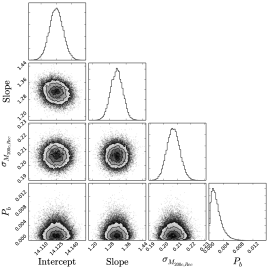
Figure 1: Example of the marginalised probability distributions produced by our MCMC analysis of the PCN method using the HOD2 catalogue for the parameters: the slope ($m$), the intercept ($c$), the scatter in the recovered mass ($\sigma_{M_{\rm Rec}}$) and the posterior fraction of data points belong to the ‘bad’ outlier distribution ($P_{\rm b}$).

We employ various statistics to examine the performance of the mass reconstruction methods including the Root Mean Square (RMS) difference between the recovered and input log mass, the scatter in the recovered mass, $\sigma_{M_{\rm Rec}}$, the scatter about the true mass $\sigma_{M_{\rm True}}$ and the bias. For the latter three statistics, we assume a model where there is a linear relationship between the recovered and true log mass and residual offsets in the recovered mass are drawn from a normal distribution. Instead of clipping outliers, we try the preferable approach of modelling the uncertainties in the data as justified in Hogg et al. (2010). We take a Bayesian approach, computing a likelihood that is a sum of the probability of obtaining the data point assuming it is drawn from a ‘good’ distribution and the probability of obtaining the data point assuming it is drawn from a ‘bad’ outlier distribution. This ensures that the measured scatter is not affected by a very small number of extreme outliers. For example, in the case of a method that produces very low scatter in general but has, say, one or two extreme outliers, the measured scatter will not be falsely inflated.

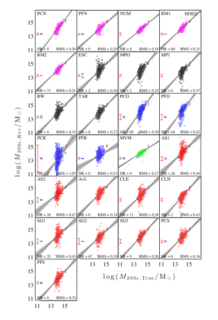
Figure 2: Recovered versus true cluster mass for the 25 methods applied to the HOD2 input catalogue. The colour scheme reflects the approach implemented by each method to deliver a cluster mass from a chosen galaxy membership: magenta (richness), black (phase space), blue (radial), green (abundance-matching) and red (velocity dispersion). The solid black line represents the fit to the recovered log mass produced by the MCMC analysis and the filled grey area presents the $\rm 3\sigma$ boundary of this fit. The red dotted line represents the 1:1 relation. ‘NR’ in the legend represents the number of missing groups/clusters. The black ticks that lie across the 1:1 relation represent the minimum and maximum ‘true’ halo $\log M_{\rm 200c}$. The vertical red bar (left) represents the mean statistical error and the vertical blue bar (right) represents the mean systematic error delivered by methods directly.

Each component of this likelihood is weighted by the probability that any given point belongs to either of these distributions:

$$\mathcal{L} \!\!\!\!=\!\!\!\! \prod_{i=1,N}p_{i}$$

$$p_{i} \!\!\!\!=\!\!\!\! \left[(1-P_{\rm b})P(\log M_{{\rm Rec},i}|\log M_{{\rm True},i},\sigma_{\log M_{{\rm Rec},i}},m,c)\right.$$ (1)

$$\qquad+\left.P_{\rm b}P(\log M_{{\rm Rec},i}|\log M_{{\rm True},i},\sigma_{\rm outlier},m,c)\right]\ .$$

Here $P_{\rm b}$ is the posterior fraction of objects belonging to the ‘bad’ outlier distribution, $\sigma_{M_{\rm Rec,i}}$ is the variance of the ‘good’ distribution and $m$, $c$ are the slope and intercept of the fit respectively, which together give the bias at any true or recovered mass. The variance of the ‘bad’ outlier distribution is fixed to be a very large number with the prior that the variance of the ‘good’ distribution must always be smaller than variance of the ‘bad’ distribution. Flat priors are adopted for the variance of the ‘good’ distribution, the slope, the intercept, while the probability that $N$ data points belong to a ‘bad’ outlier distribution must be between zero and one.

To efficiently sample our parameter space, we utilise Markov Chain Monte Carlo (MCMC) techniques that produce posterior probability distributions for these parameters. In particular, we use the parallel-tempered MCMC sampler emcee (Foreman-Mackey et al., 2013). This sampler uses several ensembles of walkers at different temperatures to explore the parameter space. A walker represents a point in the parameter space and at each iteration of the MCMC, the walkers explore by taking a randomly-sized step towards another (randomly chosen) walker i.e., towards another point in parameter space.

Each ensemble of walkers works at a certain ‘temperature’ where the likelihood is modified, enabling walkers to easily explore different local maxima i.e., preventing walkers becoming stuck at regions of local instead of global maxima in the case of a multi-modal likelihood. We employ 50 walkers at 5 temperatures and perform 2800 iterations, including a ‘burn-in’ of 1500 iterations that are discarded. In total, $50\times 5\times 2800=700\;000$ points in parameter space are sampled for each method and input catalogue. We use the autocorrelation length, which is a measure of the number of evaluations of the posterior required to produce independent samples to verify that convergence has been reached. An example of the marginalised probability distributions of the parameters produced by this parallel-tempered MCMC can be found in Figure 1. Figures of the marginalised probability distributions of parameters for all methods are available upon request.

Employing various statistics allows us to examine different aspects of the performance of the mass reconstruction methods. The RMS encompasses both scatter and bias and, hence, delivers the overall uncertainty we can expect for our ensemble of mock clusters. The scatter in the recovered mass, $\sigma_{M_{\rm Rec}}$, delivers a measure of the intrinsic scatter, i.e., in the case of no bias (a slope of unity) and no normalisation/offset. The scatter about the true mass, $\sigma_{M_{\rm True}}$, provides a measure of how well a method performs assuming there is no normalisation/offset in the relationship between recovered and true log mass. Both the scatter in the recovered mass and scatter about the true mass are useful quantities to measure when comparing methods, assuming one could accurately calibrate both the bias and normalisation/offset. The bias at the pivot mass is also calculated, where the pivot mass is taken as the median log mass of the input groups/clusters sample (log $M_{\rm 200c,true}=14.05$).

5 Results and Discussion

Now that we have described our analysis procedure, we move on to present the results of the cluster mass estimation comparison. We consider an effective method to be one that minimises scatter, has no bias in the amplitude and the slope of the relation between recovered to true mass and minimises catastrophic outliers and missing groups/clusters (whose masses cannot be determined). We therefore examine several aspects of method performance in the following subsections.

5.1 Scatter in group/cluster mass recovery

Figure 2 shows the recovered versus input log mass for the case of the HOD2 model. The colour scheme reflects the approach implemented by each method to deliver a cluster mass from a chosen galaxy membership, as introduced in Section 3. These colours are magenta (richness), black (phase space), blue (radial), green (abundance-matching) and red (velocity dispersion). Methods which select an initial cluster membership via the FOF linking method have square shaped markers, phase-space based methods have circle shaped markers and Red Sequence-based methods have diamond shaped markers.

Figure 2 clearly shows that most methods produce significant scatter for this HOD2 mock galaxy catalogue. In the case of radial based methods, we find an RMS of at least 0.39 dex up to 1.10 dex, which translates to a factor of 2.5 and 12.6 respectively. We see a better performance of phase-space and velocity dispersion -based methods -eps-converted-to.pdffor the HOD2 model where scatter is in the range of 0.26 dex up to 0.47 dex, a factor of $\sim$1.8 to 3.0.

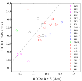
Figure 3: RMS cluster mass accuracies with the simple HOD1 input catalogue versus those derived from the more sophisticated HOD2 catalogue. The dotted black line represents a 1:1 relation. Note: PCR lies beyond the axes of this figure with an RMS of 1.07 dex for HOD2 and 0.74 dex for HOD1.

More traditional richness methods based on simply counting the number of galaxies out-perform almost all other methods based on galaxy properties using the HOD2 model.

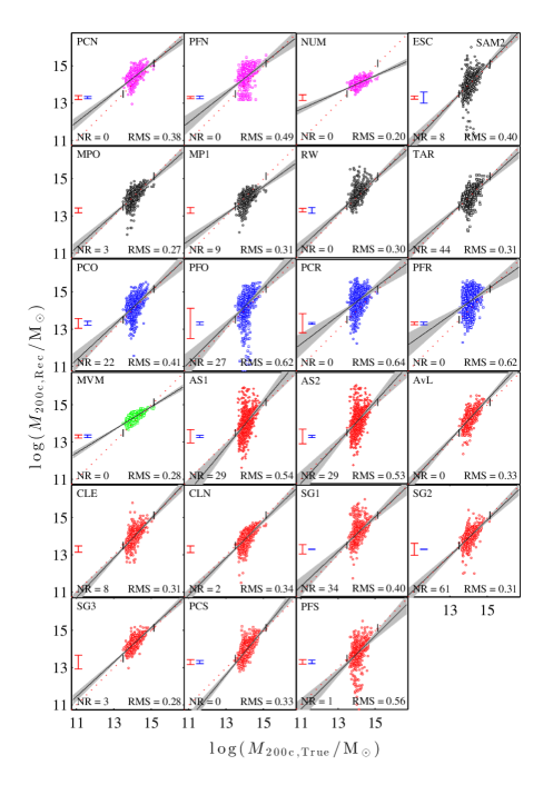
Figure 4: Recovered versus true cluster mass for the 23 methods applied to the SAM2 input catalogue. Same notation as in Figure 2.

Methods PCN, PFN, NUM, RM1 and RM2 generate much lower scatter of $\sim$0.18 – 0.26 dex and the abundance matching based method, MVM, also performs slightly better than the best richness method (NUM), producing a scatter of 0.17 dex. Note that according to Poisson statistics and the median number of galaxies in both catalogues (31), richness-based methods should produce a minimum of scatter of $\rm 1/(\sqrt{31}\ln 10)=0.08~{}dex$.

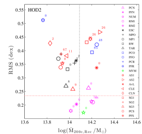
Figure 5: RMS difference in recovered versus true cluster mass versus the mean of the recovered log mass distribution, for the 25 methods applied to the HOD2 input catalogue. The dotted black line identifies where the mean of the true mass distribution lies. The red dashed line represents the RMS produced when assuming all clusters have the median true mass of the sample. The number next to each methods’ marker represents the number of groups/clusters that are not recovered because they are found to have very low ($\rm<10^{10}\,M_{\odot}$) or zero mass. Note: PCR lies beyond the axes of this figure with an RMS of 1.07 dex and $\log\bar{M}_{\rm 200c}=13.37$.

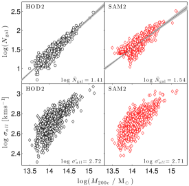
Figure B1: Upper row: richness versus mass of the 968 groups/clusters for both the HOD2 and SAM2 input catalogues. The intrinsic scatter of the richness versus mass relation of the HOD2 and SAM2 catalogue is 0.09 dex and 0.12 dex, respectively. Lower row: velocity dispersion versus mass of the 968 groups/clusters for both the HOD2 and SAM2 input catalogues. The velocity dispersion is calculated by taking the deviation of the line-of-sight velocities of all member galaxies associated with the groups/clusters. The intrinsic scatter of the velocity dispersion versus mass relation is 0.071 dex and 0.066 dex for HOD2 and SAM2, respectively. We note that this scatter is higher than Munari et al. (2013), who compute the 3D velocity dispersion, while we consider the line-of-sight velocity dispersion, which naturally results in a larger scatter, especially if the clusters are triaxial (see discussion in Mamon et al. (2010).

This can also be compared to the intrinsic scatter of both the HOD2 and SAM2 number of galaxies versus mass, shown in Figure B1. The RMS scatter in this relation is 0.09 and 0.12 dex, respectively. The recovered log mass distributions for all methods can be seen in Figure E3 along with the true log mass distributions. Figure 2 also highlights the importance of the initial galaxy selection stage of mass estimation. PCR, a method which deduces cluster mass by calculating the RMS radius of galaxies within a $\rm 1\,Mpc$ aperture and velocity range, performs poorly without any interloper removal implemented. However, PFR, a method also based on the RMS radius, is far less affected by the presence of interloping galaxies as it uses galaxies selected via FOF linking.

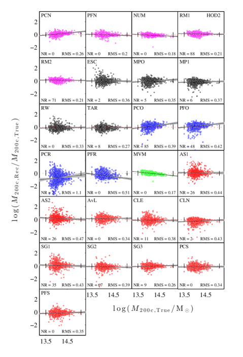
Figure E1: Residuals of the recovered versus true cluster mass for the 25 methods using the HOD2 input catalogue. This Figure follows the same notation as in Figure 2.

As expected, for the majority of methods, the RMS is higher than for Paper I, as shown Figure 3, where a catalogue based on a simple HOD model was used (HOD1). Interestingly, there are some methods (abundance matching method MVM, shifting gapper method SG2, and phase space-based methods RW and TAR) that actually have lower RMS values for the more complex HOD2 model. When we examine the residual recovered mass versus true mass for the HOD2 catalogue, shown in Figure E1, it becomes evident that the scatter is substantially higher at lower true masses, although this effect appears less severe for richness and abundance matching based methods.

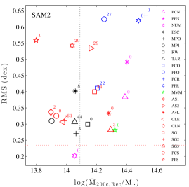
Figure 6: RMS difference in recovered versus true cluster mass versus the mean of the recovered log mass distribution, for the 23 methods applied to the SAM2 input catalogue. The dotted black line identifies where the mean of the true mass distribution lies. The red dashed line represents the RMS produced when assuming all clusters have the median true mass of the sample. The number next to each methods’ marker represents the number of groups/clusters that are not recovered because they are found to have very low ($\rm<10^{10}\,M_{\odot}$) or zero mass.

In addition to the RMS, the scatter in the recovered mass, $\rm\sigma_{M_{\rm Rec}}$, the scatter about the true mass, $\sigma_{M_{\rm True}}$, the slope and the bias at the pivot mass can be seen in Table 2 for both the HOD2 and SAM2 models. The final column of the two sub-tables shows the merit, a form of ranking based on the RMS.

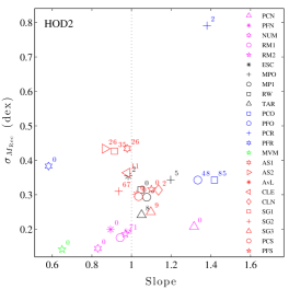
Figure 7: Scatter in the recovered cluster mass versus the slope of the fit to the recovered log mass, both delivered by the likelihood analysis, for the 25 methods applied to the HOD2 input catalogue. The dotted black line identifies a slope of unity. The number next to each methods’ marker represents the number of groups/clusters that are not recovered because they are found to have very low ($\rm<10^{10}\,M_{\odot}$) or zero mass.

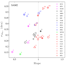
Figure 8: Scatter in the recovered cluster mass versus the slope of the fit to the recovered log mass delivered by the likelihood analysis, for the 23 methods applied to the SAM2 input catalogue. This Figure follows the same notation as in Figure 7.

It is assigned in different bins: an RMS scatter of below 0.2 dex is assigned 8 stars and then decreasing numbers of stars are assigned in subsequent bins of size 0.05 dex. The final bin of methods producing an RMS scatter greater than 0.5 dex, is given one star. In Paper I of the project, the ranking of the methods was not binned but instead, each method was assigned a rank between 1 and 23 corresponding to the lowest and highest RMS. Here, we assign a merit according to RMS bins to highlight the similarity/disparity between the scatter produced by different methods in a more linear fashion.

We see the same trends in the magnitude of the scatter for different classes of methods when we look at the scatter in the recovered mass, $\sigma_{M_{\rm Rec}}$, and the scatter about the true mass, $\sigma_{M_{\rm True}}$. According to these values, if we assume that the methods have no bias (slope of unity and zero intercept) in the relation between true and recovered mass, then they would deliver scatter as low as 0.14 – 0.15 dex (MVM and NUM respectively).

Table 2: Mass recovery accuracy (RMS, scatter in the recovered mass, $\sigma_{M_{\rm Rec}}$, slope, scatter about the true mass $\sigma_{M_{\rm True}}$ and the ranking based on $\sigma_{M_{\rm True}}$) and the bias at the pivot mass for all clusters, for both the HOD2 and SAM2 input galaxy catalogues. The merit is assigned in different bins according to the level of scatter computed by the RMS. A method producing an RMS scatter of below 0.2 dex is assigned 8 stars and then decreasing numbers of stars are assigned in subsequent bins of size 0.05 dex. The final bin of methods producing an RMS scatter greater than 0.5 dex, which is given one star.

Method	HOD2						SAM2
	RMS (dex)	$\sigma_{M_{\rm Rec}}$	Slope	$\sigma_{M_{\rm True}}$	Bias	Merit	RMS (dex)	$\sigma_{M_{\rm Rec}}$	Slope	$\sigma_{M_{\rm True}}$	Bias	Merit
PCN	0.26	0.21	1.32	0.16	$\phantom{-}0.07$	******	0.38	0.23	0.78	0.30	$\phantom{-}0.31$	****
PFN	0.20	0.20	0.89	0.22	$-0.02$	*******	0.49	0.38	0.79	0.48	$\phantom{-}0.32$	**
NUM	0.18	0.14	0.83	0.17	$-0.07$	********	0.20	0.15	0.45	0.34	$-0.01$	*******
RM1	0.21	0.18	0.94	0.19	$\phantom{-}0.12$	*******
RM2	0.21	0.19	0.97	0.19	$\phantom{-}0.11$	*******
ESC	0.36	0.35	0.98	0.36	$-0.03$	****	0.40	0.33	1.05	0.32	$-0.01$	***
MPO	0.35	0.34	1.20	0.29	$-0.05$	****	0.27	0.27	0.90	0.30	$-0.02$	******
MP1	0.37	0.29	1.08	0.27	$-0.19$	****	0.31	0.24	0.72	0.32	$-0.18$	*****
RW	0.33	0.31	1.05	0.30	$-0.11$	*****	0.30	0.29	0.92	0.32	$\phantom{-}0.05$	******
TAR	0.27	0.24	1.05	0.23	$-0.12$	******	0.31	0.31	0.91	0.34	$-0.03$	*****
PCO	0.39	0.34	1.42	0.24	$\phantom{-}0.10$	****	0.41	0.39	0.93	0.42	$\phantom{-}0.12$	***
PFO	0.42	0.34	1.33	0.26	$\phantom{-}0.15$	***	0.62	0.49	1.01	0.49	$\phantom{-}0.20$	*
PCR	1.07	0.79	1.38	0.57	$-0.73$	*	0.64	0.46	0.76	0.61	$\phantom{-}0.44$	*
PFR	0.51	0.38	0.58	0.66	$-0.31$	*	0.62	0.48	0.70	0.68	$\phantom{-}0.40$	*
MVM	0.17	0.14	0.65	0.22	$\phantom{-}0.05$	********	0.28	0.13	0.62	0.21	$\phantom{-}0.25$	******
AS1	0.44	0.43	0.98	0.44	$\phantom{-}0.10$	***	0.54	0.54	1.20	0.45	$-0.06$	*
AS2	0.47	0.43	0.87	0.50	$\phantom{-}0.19$	**	0.53	0.53	1.10	0.48	$\phantom{-}0.07$	*
AvL	0.34	0.30	1.03	0.29	$\phantom{-}0.15$	*****	0.33	0.27	1.08	0.25	$\phantom{-}0.19$	*****
CLE	0.38	0.36	0.98	0.37	$-0.11$	****	0.31	0.28	1.06	0.26	$-0.12$	*****
CLN	0.43	0.31	1.14	0.28	$-0.26$	***	0.34	0.26	0.99	0.27	$-0.19$	*****
SG1	0.43	0.43	0.91	0.47	$\phantom{-}0.07$	***	0.40	0.39	0.94	0.41	$\phantom{-}0.10$	****
SG2	0.39	0.31	0.94	0.33	$-0.15$	****	0.31	0.28	0.96	0.29	$-0.10$	*****
SG3	0.26	0.25	1.10	0.23	$-0.06$	******	0.28	0.19	0.92	0.21	$\phantom{-}0.21$	******
PCS	0.34	0.29	1.04	0.28	$-0.17$	*****	0.33	0.28	1.21	0.23	$-0.16$	*****
PFS	0.35	0.32	1.10	0.29	$-0.16$	****	0.56	0.47	0.99	0.47	$-0.29$	*

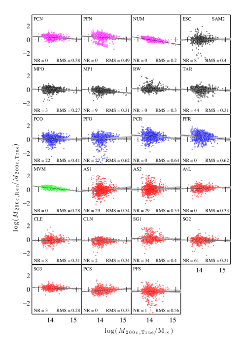
Figure E2: Residuals of the recovered versus true cluster mass for the 23 methods applied to the SAM2 input catalogue. This Figure follows the same notation as in Figure E1.

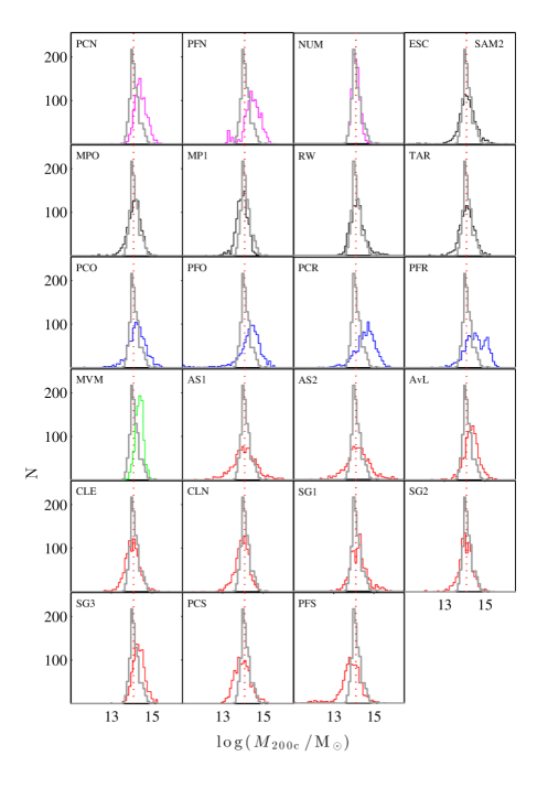
Figure E4: Recovered mass distributions for the 23 methods applied to the SAM2 input catalogue. This Figure follows the same notation as in Figure E3.

Now that we have examined the results for the sophisticated HOD2 catalogue, we move on to examine how well the cluster mass reconstruction methods perform using the SAM2. Figure 4 shows the recovered log mass versus input log mass for 23 participating methods. Note that methods RM1 and RM2 did not participate as the method could not run on the catalogue due to the less prominent Red Sequence produced by the SAM2 model. Immediately, we see high levels of scatter for almost all methods with the exception of NUM. Furthermore, as we saw with the HOD2 catalogue, this scatter appears significantly worse at lower group/cluster masses when we look at the residual recovered mass in Figure E2. Exceptions are for methods NUM, MP1, TAR and especially PFO, whose scatter is lower at the low-mass end (though is still comparably large)! Not only does this show that the scatter is dependent on the true group/cluster mass but it also suggests that this mass dependence is not consistent across all methods. This is confirmed when we examine the values of scatter produced when the sample is split into lower and higher mass groups/clusters, as shown in Tables C1 and C2 in the appendix. This implies that if one had prior knowledge of whether a sample of objects contained either groups or high mass clusters (e.g., from other cluster mass proxies), then more accurate masses would be obtained if a method that performed best for that mass category were chosen, as opposed to a method with lower scatter over the entire mass range. The recovered log mass distributions for all methods can be seen in Figure E4 along with the true log mass distributions.

One can compare the scatter found for MPO and MP1 with the scatter found by Mamon et al. (2013) when they tested this method on mock projected phase space distributions derived from random sampling of the dark matter particle distribution in haloes of hydrodynamical cosmological simulations. Indeed, Mamon et al. (2013) found a scatter of 0.040 and 0.058 dex in log $R_{\rm 200c}$ for samples of 500 and 100 galaxies, which respectively amount to 0.12 and 0.17 dex for log $M_{\rm 200c}$. In the present study, limited to the higher mass haloes, MPO and MP1 achieve 0.28 and 0.23 dex scatter with the HOD2 groups/clusters (Table C1), and 0.22 and 0.21 dex scatter with SAM2 groups/clusters (Table C2). Given that the present study uses, on average, lower numbers of galaxies per halo of 38 (HOD2) and 53 (SAM2) for the high-mass subsamples, our values appear consistent with the scatter values of Mamon et al. (2013). Similarly, the RW model has been tested by Wojtak et al. (2009), to yield 0.13 dex for 300 particle haloes, while in the present study limited to high-mass clusters, RW achieves scatter of 0.27 and 0.26 dex for HOD2 (Table C1) and SAM2 (Table C2), respectively.

It is also useful to evaluate the effectiveness of using colours to evaluate the virial masses. For example, the methodology used in MP1 is identical to that of MPO, except that the former is colour-blind. Table 2 indicates that MPO and MP1 have comparable accuracies in mass recovery: for the HOD2 and SAM2 samples, MPO has a scatter 0.05 and 0.01 dex higher than MP1, but an RMS that is 0.03 and 0.09 dex lower. In other words, the colour information helps to reduce the bias, but not the scatter.

5.2 Bias in group/cluster mass recovery

The methods do not collectively under- or over-estimate the mean true mass for the HOD2 groups/clusters, as shown in Figure 5. With the exception of radial-based techniques, the methods are clustered around the true mean log mass. Interestingly, this agreement was not seen in Paper I when the methods systematically underestimated the mean log mass when tested with the more simple HOD1 model. We do not see this underestimation with the more sophisticated HOD2 model as the calibration of velocity dispersions as a function of halo mass and radius is updated and the treatment galaxy dynamics (which affect the spatial and redshift distributions) is slightly modified. Figure 5 also indicates that there is no strong correlation between the mean recovered mass and scatter produced by the methods.

A measure of the bias at the pivot mass, which reflects the bias in the amplitude of the relation between recovered and true log mass, is shown in Table 2. For the HOD2 catalogue, it is clear that low levels of bias can be produced by many methods: PFN and ESC produce a bias of $\leq\pm 0.03$ whilst other methods MPO, MVM produce a bias of $\leq\pm 0.05$. Within method classes we see a wide range of these bias values.

For the SAM2 catalogue, we also see that the methods do not collectively under- or over-estimate the mean true mass for the SAM2 groups/clusters, as shown in Figure 6. We do however, see slightly larger values in the bias at the pivot mass, although methods NUM, ESC, MPO, RW and TAR produce a bias of $\leq\pm 0.05$. As with the HOD catalogue, we see a wide range of these bias values within method classes. Figures 7 and 8 and the result of a Spearman rank test show that scatter is uncorrelated with slope of the recovered and input mass relation for the HOD2 model, however, the scatter is marginally correlated with the slope for the SAM2 (with a p-value = 0.0549). Surprisingly, MVM, an abundance matching based method with very low scatter in the recovered mass, has a low slope of 0.65. This flatter slope artificially boosts the scatter about the true mass, as we can see from the values in Table 2. The scatter in the recovered mass is 0.14 dex as opposed to for the scatter about the true mass. This suggests that if MVM were able to produce a slope equal to unity, the scatter in for this method would be as low as 0.14 dex.

It is important to understand how our results vary due to the underlying model used to produce the catalogue. As touched on above, we see some differences in the recovered masses for different classes of methods using two very different input mock galaxy catalogues. Though we see some differences method-to-method, collectively, the methods do not systematically have substantially higher scatter or more bias in the slope or amplitude for either model.

This is especially clear in Figure 9 and Figure 10 where histograms of the RMS and scatter about the true mass are shown for all methods and each model. There is a surprising similarity between the RMS and scatter in the recovered mass for both the HOD2 and SAM2 models for many methods. This is encouraging, as it suggests that either the galaxy population produced by these two contrasting models is analogous or the methods are insensitive to the differences between these models.

5.3 Catastrophic outliers and missing clusters

When we examine the performance of these methods, it is clear that there are a number of groups/clusters whose masses are either greatly under- or over-estimated. For example, in the HOD2 catalogue, there are three clusters with mass greater than $\rm 10^{15}\,M_{\odot}$, but some methods predict many more clusters with such large masses (e.g., PCO (39), AS1 (52), AS2 (54) and SG1 (42), see Figure E4). Obtaining the correct number of high mass clusters is crucial for studies selecting high mass clusters – given the steeply falling mass function at the high mass end, even a small number of false high mass cluster measurements would have a large impact.

Furthermore, significant underestimations of mass is also very detrimental, as cosmological constraining power increases with lower mass clusters (as signal to noise increases with decreasing mass). For this reason, it is important to assess the fraction of groups/clusters for which a method under- or over-estimates the mass by a large factor. The percentage of groups/clusters whose mass is under- or over-estimated by a factor of 10 is shown for all methods and each model in the form of histograms in Figure 11. Groups/clusters whose masses are over-estimated by over a factor of 10 are shown as a positive percentage and those whose are underestimated by over a factor of 10 are shown as a negative percentage. The percentage of groups/clusters that are missing i.e., no mass was found for these objects, is shown in white. Encouragingly, richness-based methods PCN, NUM, RM1, RM2 and abundance-based method MVM have extremely low fraction of these failures.

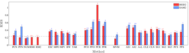
Figure 9: Histogram of the RMS of the difference between the recovered and true cluster masses (in $\rm dex$) for all methods applied to the HOD2 (red) and SAM2 (blue) input catalogues. The black dashed line represents the RMS produced when we assume all clusters have the same mass. This uniform mass is chosen to be the mean input log mass. The number above each bar represents the number of missing groups/clusters.

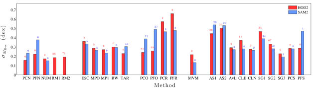
Figure 10: Histogram of the scatter in the recovered cluster mass (in $\rm dex$) for all methods using the HOD2 (red) and SAM2 (blue) input catalogues. The number above each bar represents the number of missing groups/clusters.

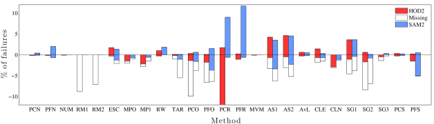
Figure 11: Histogram of the percentage of groups/clusters whose recovered mass is over-estimated (positive $\%$) or underestimated (negative $\%$) by a factor of ten or more relative to the true mass for all methods applied to the HOD2 (red) and SAM2 (blue) input catalogues. The white segments of each bar represents the number of missing groups/clusters. Note that the y-axis of this plot is truncated so that detail at the low percentage range is seen more clearly. PCR falls below this truncation with $32.1\%$ of group/cluster masses underestimated by a factor of ten.

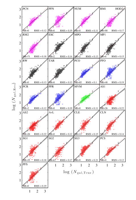
Figure 12: Recovered versus true cluster richness for the 25 methods run on the HOD2 input catalogue. The colour scheme reflects the approach implemented by each method to deliver a cluster mass from a chosen galaxy membership: magenta (richness), black (phase space), blue (radial), green (abundance-matching) and red (velocity dispersion). The solid black line represents the fit to the recovered $N_{\rm gal}$ produced by the MCMC analysis and the filled grey area presents the $\rm 3\sigma$ boundary of this fit. The red dotted line represents the 1:1 relation. ‘NR’ in the legend represents the number of missing groups/clusters. The black ticks that lie across the 1:1 relation represent the minimum and maximum ‘true’ halo $N_{\rm gal}$.

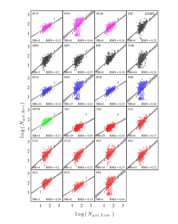
Figure 13: Recovered versus true cluster richness for the 23 methods run on the SAM2 input catalogue. This Figure follows the same notation as in Figure 12.

However, some radial-based and velocity dispersion based methods predict masses out by over a factor of 10 for over $\rm 50$ groups/clusters (i.e., 5%). This result indicates that if these velocity dispersion, radial-based or phase space -based methods are used, it is vital to also apply abundance matching or certain richness based techniques as a sanity check to ensure there are no catastrophic failures that would misrepresent the shape of the mass function.

The fraction of groups/clusters whose masses are not recovered are shown as white segments in Figure 11. We see a large variation between methods, but no correlation of the fraction of missing clusters with method class. Methods such as RM1, RM2, TAR, PCO, PFO and SG2 do not recover masses for $\rm 4-8\%$ of groups/clusters, whereas many methods recover masses for all clusters e.g., PCN, PFN, NUM, PCR, PFR, MVM, AvL, PCS and PFS.

5.4 Group/cluster $N_{\rm gal}$ recovery

In this section, we present the results of the number of galaxies (i.e., the richness) recovered by the cluster mass reconstruction techniques using both the more sophisticated HOD2 and SAM2 input galaxy catalogues. Figures 12 and 13 show the recovered log number of galaxies versus input log number of galaxies for the case of the HOD2 model and SAM2 model respectively. The colour scheme, lines, symbols and statistics are the same as for the mass comparison figures.

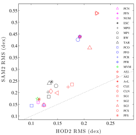
Figure 14: RMS cluster richness errors from the 23 methods applied to the SAM2 input catalogue versus those found when applied to the HOD2 input catalogue. The dotted black line represents a 1:1 relation.

In general, we see a stronger correlation of the recovered richness to the input richness and lower RMS values for the methods for both the HOD2 and SAM2 catalogues in comparison with group/cluster mass. The mean RMS values produced by methods using both catalogues are 0.31 dex for mass estimation and 0.21 dex for $N_{\rm gal}$ estimation respectively. This is also highlighted in Figure 14, which shows the RMS difference between the recovered and input log $N_{\rm gal}$ for the SAM2 catalogue versus the HOD2 catalogue and Table D1, which shows this RMS, as well as the scatter in the recovered richness, $\sigma_{N_{\rm Rec}}$, the scatter about the true richness, $\sigma_{N_{\rm True}}$, the slope and the bias at the pivot number of galaxies.

Again, we see very low RMS values for NUM, MVM and radial-based method PCO for the HOD2 catalogue. The outliers with higher RMS values for the SAM2 catalogue are PFN, PFO, PFR and PFS, methods that select an initial galaxy membership list via FOF. Red Sequence based methods AS1 and AS2, also have a very high RMS values, though, this is mostly due to the large bias observed at the pivot mass (-0.48 dex). It is evident from Figure 14 that all methods have lower scatter in the true number of galaxies for the HOD2 input catalogue in comparison with for the SAM2 input catalogue. This is not unexpected, as it is the nature of the HOD2 model to deliver groups/clusters that have a very strong mass – richness correlation. Interestingly though, this strong boost in scatter for the SAM2 catalogue does not necessarily translate to a much larger scatter in the mass, as reflected in Figure 9.

Now that we have examined the level of scatter for the recovered richness, we move on to look at the bias. From Table D1, we see slopes of $\rm<1$ for the SAM2 catalogue but we do not see the same behaviour for the HOD2 model and, as in the case of the scatter, this does not translate to a systematic shallower slope for the recovered mass. It is important to note that the slope of the $N_{\rm gal}$ – $M_{\rm 200c}$ relation is lower in the SAM2 as shown in Figure B1. We also find that the recovered richness versus recovered mass is as found in Paper I, where the richness-based methods, have, as expected, very tight relations. In contrast, many other methods have more scatter in both recovered number and recovered mass. Note that recovering the correct number of galaxies does not necessarily guarantee that the correct member galaxies are being recovered. The fact that we see substantially lower scatter in the recovered number of galaxies but not the mass, indicates that it is not sufficient to simply obtain the correct number of galaxies. To deliver low scatter, it is essential to get the correct membership.

6 Conclusions

We have performed an extensive test of 25 different galaxy-based cluster mass reconstruction methods by using two contrasting mock galaxy catalogues that are produced using sophisticated, observationally realistic HOD2 and SAM2 models, run on the same halo merger tree extracted from the same cosmological $N$-body simulation. The aim of this work is to determine the level of scatter, the bias and completeness that these methods produce, giving insight into how we can improve on these techniques while generating more realistic mock galaxy catalogues. The main results are as follows:

1. Phase-space and velocity dispersion -based methods deliver a similar level of RMS scatter within the range of a factor of $\sim$1.8 – 3, whilst radial-based methods perform significantly worse, delivering an RMS scatter of within a factor of $\sim$2.5 – 12.

2. Richness based methods produce a comparably lower level of RMS scatter within the range of a factor of $\sim$1.5 – 3.1. The lower RMS scatter produced by richness based methods for both HOD2 and SAM2 mock catalogues (where different assumptions are employed to populate dark matter haloes with galaxies) suggest that the good performance of these methods is robust. The abundance matching-based technique we tested also produces a comparably lower level of RMS scatter within the range of a factor of $\sim$1.5 – 1.9 for both models.

3. For many, but not all methods, we find that the scatter is group/cluster mass-dependent and the direction of this dependence varies across methods.

4. As expected, for the majority of methods, the scatter is higher than for Paper I, where 23 methods were tested on a catalogue based on a simple HOD model. Though, interestingly, there are four methods that have lower RMS values for the more complex HOD2 model.

5. We see a large variation of bias in the slope of the recovered and input mass relation across all methods for both the HOD2 and SAM2 galaxy catalogues.

6. Many methods produce a significant number of catastrophic failures, where group/cluster masses are over or under -estimated by a factor of $\geq 10$. For studies selecting high mass clusters, these failures can be detrimental due to the steeply falling high-mass end of the cluster mass function. For this reason, we recommend that richness or abundance matching -based methods are used as a sanity check in conjunction with phase-space, velocity dispersion or radial -based methods when high cluster masses are recovered.

7. We see a stronger correlation of the recovered to input number of galaxies for both catalogues in comparison with recovered to input group/cluster mass. The mean RMS produced by methods using both catalogues 0.31 dex for mass estimation and 0.21 dex for $N_{\rm gal}$ estimation. However, this does not mean the correct member galaxies are being selected. The boost in scatter from the number of galaxies to mass indicates that the selection of the correct galaxies (and not just the correct number of galaxies) is a key to delivering lower scatter for these methods.

8. We see a variation of bias in the slope of the recovered and input number of galaxies relation across all methods for the HOD2, however, all methods produce a slope of less than unity for the SAM2 galaxy catalogue.

9. Though we see some differences method-to-method, in general, methods do not have significantly higher scatter for either the more sophisticated HOD2 or the SAM2 galaxy catalogues. This is encouraging, as it suggests that either the galaxy population produced by these two contrasting models is analogous or the methods are insensitive to the differences between these models.

There are several outstanding questions that we hope to address in future using our dataset. What is the impact of observational limitations such as fibre collisions or survey artifacts on group/cluster membership and hence mass recovery? What is the impact of halo shape and concentration on group/cluster mass recovery (Wojtak et al. in preparation)? What produces the catastrophic under- or over- estimates in each of the 25 methods? These projects share the overall goal of improving or constructing more accurate cluster mass reconstruction techniques.

Appendix A Properties of the Mass Reconstruction Methods

Table 3: Illustration of the member galaxy selection process for all methods. The second column details how each method selects an initial member galaxy sample, while the third column outlines the member galaxy sample refining process. Finally, the fourth column describes how methods treat interloping galaxies that are not associated with the clusters.

Methods	Member galaxy selection methodology
	Initial Galaxy Selection	Refine Membership	Treatment of Interlopers
PCN	Within $\rm 5\,Mpc$, $\rm 1000\,km\,s^{-1}$	Clipping of $\pm 3\,\sigma$, using galaxies within $\rm 1\,Mpc$	Use galaxies at $\rm 3-5\,Mpc$ to find interloper population to remove
PFN	FOF	No	No
NUM	Within $\rm 3\,Mpc$, $\rm 4000\,km\,s^{-1}$	1) Estimate $R_{\rm 200c}$ from the relationship between $R_{\rm 200c}$ and richness deduced from CLE; 2) Select galaxies within $R_{\rm 200c}$ and with $|v|<2.7\,\sigma_{\rm los}^{\rm NFW}(R)$	No
RM1	Red Sequence	Red Sequence	Probabilistic
RM2	Red Sequence	Red Sequence	Probabilistic
ESC	Within preliminary $R_{\rm 200c}$ estimate and $\rm\pm 3500\,km\,s^{-1}$	Gapper technique	Removed by Gapper technique
MPO	Input from CLN	1) Calculate $R_{\rm 200c}$ , $R_{\rm\rho}$, $R_{\rm red}$, $R_{\rm blue}$ by MAMPOSSt method; 2) Select members within radius according to colour	No
MP1	Input from CLN	Same as MPO except colour blind	No
RW	Within $\rm 3\,\,Mpc$, $\rm 4000\,\,km\,s^{-1}$	Within $R_{\rm 200c}$ , $|2\Phi(R)|^{1/2}$, where $R_{\rm 200c}$ obtained iteratively	No
TAR	FOF	No	No
PCO	Input from PCN	Input from PCN	Include interloper contamination in density fitting
PFO	Input from PFN	Input from PFN	No
PCR	Input from PCN	Input from PCN	Same as PCN
PFR	Input from PFN	Input from PFN	No
MVM	FOF (ellipsoidal search range, centre of most luminous galaxy)	Increasing mass limits, then FOF, loops until closure condition	No
AS1	Within $\rm 1\,Mpc$, $\rm 4000\,km\,s^{-1}$, constrained by colour-magnitude relation	Clipping of $\pm 3\,\sigma$	Removed by clipping of $\pm 3\,\sigma$
AS2	Within $\rm 1\,Mpc$, $4\rm 000\,km\,s^{-1}$, constrained by colour-magnitude relation	Clipping of $\pm 3\,\sigma$	Removed by clipping of $\pm 3\,\sigma$
AvL	Within $2.5\,\sigma_{v}$ and $0.8\,R_{\rm 200}$	Obtain $R_{\rm 200c}$ and $\,\sigma_{v}$ by $\,\sigma$-clipping	No
CLE	Within $\rm 3\,Mpc$, $\rm 4000\,km\,s^{-1}$	1) Estimate $R_{\rm 200c}$ from the aperture velocity dispersion; 2) Select galaxies within $R_{\rm 200c}$ and with $|v|<2.7\,\sigma_{\rm los}^{\rm NFW}(R)$; 3) Iterate steps 1 and 2 until convergence	Obvious interlopers are removed by velocity gap technique, then further treated in iteration by $\sigma$ clipping
CLN	Input from NUM	Same as CLE	Same as CLE
SG1	Within $\rm 4000\,km\,s^{-1}$	1) Measure $\,\sigma_{\rm gal}$, estimate $M_{\rm 200c}$ and $R_{\rm 200c}$ ; 2) Select galaxies within $R_{\rm 200c}$ ; 3) Iterate steps 1 and 2 until convergence	Shifting gapper with minimum bin size of $\rm 250\,kpc$ and 15 galaxies; velocity limit $\rm 1000\,km\,s^{-1}$ from main body
SG2	Within $\rm 4000\,km\,s^{-1}$	1) Measure $\sigma_{\rm gal}$, estimate $M_{\rm 200c}$ and $R_{\rm 200c}$ ; 2) Select galaxies within $R_{\rm 200c}$ ; 3) Iterate steps 1 and 2 until convergence	Shifting gapper with minimum bin size of $\rm 150\,kpc$ and 10 galaxies; velocity limit $\rm 500\,km\,s^{-1}$ from main body
SG3	Within $\rm 2.5\,h^{-1}\,Mpc$ and $\rm 4000\,km\,s^{-1}$. Velocity distribution symmetrized	Measure $\,\sigma_{\rm gal}$, correct for velocity errors, then estimate $M_{\rm 200c}$ and $R_{\rm 200c}$ and apply the surface pressure term correction	Shifting gapper with minimum bin size of $\rm 420\,h^{-1}kpc$ and 15 galaxies
PCS	Input from PCN	Input from PCN	Same as PCN
PFS	Input from PFN	Input from PFN	No

Table A2: Characteristics of the mass reconstruction process of methods used in this comparison. The second, third, fourth and fifth columns illustrate whether a method calculates/utilises the velocities, velocity dispersion, radial distance of galaxies from cluster centre, the richness and the projected phase space information of galaxies respectively. If a method assumed a mass or number density profile it is indicated in columns six and seven.

Methods	Galaxy properties used to obtain group/cluster membership and estimate mass
	Velocities	Velocity dispersion	Radial distance	Richness	Projected phase space	Mass density profile	Number density profile
PCN	Yes	No	No	Yes	No	No	No
PFN	Yes	No	No	Yes	No	No	No
NUM	No	No	No	Yes	Yes	No	No
RM1	No	No	Yes	Yes	No	No	NFW
RM2	No	No	Yes	Yes	No	No	NFW
ESC	Yes	Yes	Yes	No	No	Caustics	No
MPO	Yes	No	Yes	No	Yes	NFW	Yes
MP1	Yes	No	Yes	No	Yes	NFW	Yes
RW	Yes	No	Yes	No	Yes	NFW	Yes
TAR	Yes	Yes	Yes	No	No	NFW	No
PCO	Yes	No	No	No	No	NFW	Yes
PFO	Yes	No	No	No	No	NFW	Yes
PCR	Yes	No	Yes	No	No	No	No
PFR	Yes	No	Yes	No	No	No	No
MVM	Yes	Yes	Yes	No	No	NFW	No
AS1	Yes	Yes	No	No	No	No	No
AS2	Yes	No	Yes	No	Yes	No	No
AvL	Yes	Yes	Yes	No	No	No	No
CLE	Yes	Yes	No	No	No	NFW	NFW
CLN	Yes	Yes	No	No	No	NFW	NFW
SG1	Yes	Yes	Yes	No	No	No	No
SG2	Yes	Yes	Yes	No	No	No	No
SG3	Yes	Yes	Yes	No	No	No	No
PCS	Yes	Yes	No	No	No	No	No
PFS	Yes	Yes	No	No	No	No	No

Appendix B: Richness and velocity dispersion – mass relations

Appendix C: Mass recovery accuracy for low and high group/cluster samples

Table C1: Mass recovery accuracy (RMS, scatter in the recovered mass ($\sigma_{M_{\rm Rec}}$), slope, scatter about the true mass ($\sigma_{M_{\rm True}}$) and the ranking based on $\sigma_{M_{\rm True}}$) for low- and high-mass clusters (split according to the median true mass in each subsample) for the HOD2 input catalogue. A method producing an RMS scatter of below 0.2 dex is assigned 8 stars and then decreasing numbers of stars are assigned in subsequent bins of size 0.05 dex. The final bin of methods producing an RMS scatter greater than 0.5 dex, is given one star

Method	HOD2 low masses						HOD2 high masses
	RMS (dex)	$\sigma_{M_{\rm Rec}}$	Slope	$\sigma_{M_{\rm True}}$	Bias	Merit	RMS (dex)	$\sigma_{M_{\rm Rec}}$	Slope	$\sigma_{M_{\rm True}}$	Bias	Merit
PCN	0.23	0.23	1.21	0.19	$\phantom{-}0.03$	*******	0.29	0.18	1.28	0.14	$\phantom{-}0.14$	******
PFN	0.21	0.21	0.79	0.27	$-0.01$	*******	0.19	0.18	0.94	0.19	$-0.04$	********
NUM	0.17	0.16	0.72	0.22	$-0.06$	********	0.19	0.13	0.82	0.16	$-0.09$	********
RM1	0.22	0.18	0.57	0.32	$\phantom{-}0.11$	*******	0.20	0.17	0.99	0.17	$\phantom{-}0.11$	********
RM2	0.23	0.20	0.55	0.37	$\phantom{-}0.09$	*******	0.20	0.17	1.00	0.17	$\phantom{-}0.11$	********
ESC	0.44	0.44	0.78	0.57	$-0.02$	***	0.26	0.26	1.16	0.22	$-0.05$	******
MPO	0.40	0.39	1.28	0.31	$-0.07$	****	0.30	0.28	1.17	0.24	$-0.01$	*****
MP1	0.41	0.34	1.07	0.32	$-0.20$	***	0.33	0.23	1.07	0.22	$-0.17$	*****
RW	0.37	0.35	1.24	0.28	$-0.10$	****	0.29	0.27	1.07	0.25	$-0.11$	******
TAR	0.31	0.27	1.01	0.27	$-0.14$	*****	0.23	0.21	0.99	0.21	$-0.10$	*******
PCO	0.44	0.42	1.48	0.29	$\phantom{-}0.03$	***	0.35	0.29	1.43	0.20	$\phantom{-}0.17$	*****
PFO	0.47	0.40	1.60	0.25	$\phantom{-}0.12$	**	0.37	0.27	1.31	0.21	$\phantom{-}0.20$	****
PCR	1.28	0.97	0.93	1.04	$-0.84$	*	0.82	0.56	0.99	0.56	$-0.60$	*
PFR	0.49	0.42	0.45	0.94	$-0.26$	**	0.53	0.34	0.63	0.54	$-0.39$	*
MVM	0.19	0.16	0.59	0.26	$\phantom{-}0.08$	********	0.16	0.13	0.61	0.20	$-0.00$	********
AS1	0.50	0.49	1.10	0.45	$\phantom{-}0.11$	**	0.38	0.37	1.02	0.37	$\phantom{-}0.08$	****
AS2	0.53	0.49	0.99	0.49	$\phantom{-}0.21$	*	0.40	0.38	0.92	0.41	$\phantom{-}0.15$	***
AvL	0.38	0.34	1.09	0.32	$\phantom{-}0.16$	****	0.29	0.25	1.08	0.23	$\phantom{-}0.15$	******
CLE	0.43	0.42	1.08	0.39	$-0.09$	***	0.33	0.30	1.11	0.27	$-0.14$	*****
CLN	0.48	0.36	1.27	0.28	$-0.28$	**	0.37	0.25	1.11	0.22	$-0.23$	****
SG1	0.50	0.50	1.11	0.45	$\phantom{-}0.10$	*	0.35	0.35	0.99	0.35	$\phantom{-}0.03$	*****
SG2	0.45	0.36	0.97	0.37	$-0.14$	**	0.32	0.24	1.00	0.24	$-0.18$	*****
SG3	0.29	0.28	1.08	0.26	$-0.08$	******	0.22	0.21	1.05	0.20	$-0.04$	*******
PCS	0.37	0.33	1.09	0.30	$-0.16$	****	0.31	0.26	1.13	0.23	$-0.18$	*****
PFS	0.37	0.34	1.42	0.24	$-0.15$	****	0.33	0.27	1.14	0.24	$-0.15$	*****

Table C2: Mass recovery accuracy for low and high mass groups/SAM2 clusters. Same notation as Table C1.

Method	SAM2 low masses						SAM2 high masses
	RMS (dex)	$\sigma_{M_{\rm Rec}}$	Slope	$\sigma_{M_{\rm True}}$	Bias	Merit	RMS (dex)	$\sigma_{M_{\rm Rec}}$	Slope	$\sigma_{M_{\rm True}}$	Bias	Merit
PCN	0.41	0.23	0.12	$\phantom{-}1.96$	$\phantom{-}0.31$	***	0.35	0.22	0.90	$\phantom{-}0.25$	$\phantom{-}0.27$	*****
PFN	0.51	0.37	0.26	$\phantom{-}1.41$	$\phantom{-}0.34$	*	0.47	0.38	0.97	$\phantom{-}0.40$	$\phantom{-}0.28$	**
NUM	0.19	0.15	0.03	$-5.41$	$\phantom{-}0.03$	********	0.22	0.15	0.50	$\phantom{-}0.30$	$-0.10$	*******
ESC	0.42	0.41	1.13	$\phantom{-}0.36$	$-0.02$	***	0.38	0.26	1.08	$\phantom{-}0.24$	$-0.01$	****
MPO	0.31	0.31	1.01	$\phantom{-}0.30$	$-0.01$	*****	0.23	0.22	0.89	$\phantom{-}0.25$	$-0.04$	*******
MP1	0.30	0.26	0.79	$\phantom{-}0.33$	$-0.14$	******	0.32	0.21	0.71	$\phantom{-}0.29$	$-0.22$	*****
RW	0.34	0.33	0.89	$\phantom{-}0.37$	$\phantom{-}0.06$	*****	0.26	0.26	0.95	$\phantom{-}0.27$	$\phantom{-}0.04$	******
TAR	0.30	0.30	0.37	$\phantom{-}0.79$	$-0.03$	*****	0.31	0.31	1.09	$\phantom{-}0.28$	$-0.06$	*****
PCO	0.41	0.38	0.06	$-6.36$	$\phantom{-}0.11$	***	0.41	0.38	1.30	$\phantom{-}0.29$	$\phantom{-}0.09$	***
PFO	0.60	0.46	0.13	$\phantom{-}3.53$	$\phantom{-}0.20$	*	0.64	0.57	1.49	$\phantom{-}0.38$	$\phantom{-}0.13$	*
PCR	0.71	0.54	0.70	$\phantom{-}0.77$	$\phantom{-}0.45$	*	0.56	0.37	0.60	$\phantom{-}0.62$	$\phantom{-}0.43$	*
PFR	0.67	0.50	0.37	$\phantom{-}1.35$	$\phantom{-}0.42$	*	0.57	0.46	0.75	$\phantom{-}0.60$	$\phantom{-}0.35$	*
MVM	0.33	0.14	0.74	$\phantom{-}0.19$	$\phantom{-}0.29$	*****	0.22	0.12	0.55	$\phantom{-}0.22$	$\phantom{-}0.19$	*******
AS1	0.63	0.62	1.23	$\phantom{-}0.51$	$-0.08$	*	0.45	0.45	1.30	$\phantom{-}0.34$	$-0.04$	***
AS2	0.62	0.62	1.18	$\phantom{-}0.52$	$\phantom{-}0.06$	*	0.44	0.44	1.20	$\phantom{-}0.36$	$\phantom{-}0.07$	***
AvL	0.35	0.30	1.27	$\phantom{-}0.24$	$\phantom{-}0.19$	****	0.31	0.24	1.12	$\phantom{-}0.22$	$\phantom{-}0.19$	*****
CLE	0.33	0.31	1.32	$\phantom{-}0.24$	$-0.11$	*****	0.28	0.25	1.07	$\phantom{-}0.24$	$-0.11$	******
CLN	0.37	0.30	1.14	$\phantom{-}0.26$	$-0.18$	****	0.31	0.24	1.00	$\phantom{-}0.24$	$-0.19$	*****
SG1	0.46	0.45	0.96	$\phantom{-}0.47$	$\phantom{-}0.11$	**	0.33	0.32	0.95	$\phantom{-}0.34$	$\phantom{-}0.08$	*****
SG2	0.33	0.32	1.26	$\phantom{-}0.25$	$-0.07$	*****	0.29	0.24	1.01	$\phantom{-}0.24$	$-0.12$	******
SG3	0.30	0.21	0.89	$\phantom{-}0.24$	$\phantom{-}0.21$	*****	0.26	0.18	0.93	$\phantom{-}0.19$	$\phantom{-}0.20$	******
PCS	0.36	0.31	1.23	$\phantom{-}0.25$	$-0.18$	****	0.28	0.25	1.27	$\phantom{-}0.20$	$-0.14$	******
PFS	0.56	0.49	0.78	$\phantom{-}0.63$	$-0.28$	*	0.55	0.44	1.17	$\phantom{-}0.38$	$-0.31$	*

Appendix D: Richness recovery

Table D1: The RMS, scatter in the observed richness, $\sigma_{N_{\rm gal,obs}}$, slope, scatter about the true richness $\sigma_{N_{\rm gal,true}}$ and the bias at the pivot richness (for the HOD2: log $N_{\rm gal,true}=1.41$ and for the SAM2: log $N_{\rm gal,true}=1.54$).

Method	HOD2					SAM2
	RMS (dex)	$\sigma_{N_{\rm gal,obs}}$	Slope	$\sigma_{N_{\rm gal,true}}$	Bias	RMS (dex)	$\sigma_{N_{\rm gal,obs}}$	Slope	$\sigma_{N_{\rm gal,true}}$	Bias
PCN	0.12	0.09	0.86	0.10	$\phantom{-}0.00$	0.15	0.12	0.62	0.19	$-0.00$
PFN	0.19	0.17	0.92	0.18	$\phantom{-}0.09$	0.44	0.35	0.89	0.39	$\phantom{-}0.27$
NUM	0.11	0.10	0.97	0.10	$\phantom{-}0.02$	0.16	0.15	0.77	0.19	$\phantom{-}0.04$
RM1	0.17	0.14	0.95	0.15	$-0.08$
RM2	0.18	0.15	0.98	0.15	$-0.09$
ESC	0.14	0.14	0.94	0.14	$\phantom{-}0.03$	0.25	0.20	0.90	0.23	$\phantom{-}0.03$
MPO	0.13	0.12	1.05	0.12	$-0.04$	0.20	0.19	0.89	0.21	$-0.07$
MP1	0.15	0.13	1.03	0.13	$-0.07$	0.23	0.19	0.84	0.23	$-0.11$
RW	0.13	0.13	0.98	0.13	$\phantom{-}0.00$	0.18	0.18	0.88	0.20	$\phantom{-}0.02$
TAR	0.13	0.13	0.94	0.14	$\phantom{-}0.01$	0.24	0.24	0.90	0.26	$\phantom{-}0.04$
PCO	0.10	0.09	0.85	0.11	$\phantom{-}0.01$	0.14	0.12	0.61	0.19	$\phantom{-}0.00$
PFO	0.19	0.16	0.90	0.18	$\phantom{-}0.10$	0.43	0.32	0.91	0.35	$\phantom{-}0.29$
PCR	0.12	0.09	0.86	0.10	$\phantom{-}0.00$	0.15	0.12	0.62	0.19	$-0.00$
PFR	0.19	0.17	0.92	0.18	$\phantom{-}0.09$	0.44	0.35	0.89	0.39	$\phantom{-}0.27$
MVM	0.11	0.09	0.77	0.11	$\phantom{-}0.02$	0.17	0.12	0.63	0.18	$\phantom{-}0.12$
AS1	0.22	0.17	0.78	0.22	$-0.13$	0.54	0.15	0.56	0.27	$-0.48$
AS2	0.22	0.17	0.78	0.22	$-0.13$	0.54	0.15	0.56	0.27	$-0.48$
AvL	0.12	0.11	0.97	0.11	$\phantom{-}0.01$	0.17	0.17	0.92	0.19	$\phantom{-}0.01$
CLE	0.15	0.15	0.99	0.15	$\phantom{-}0.01$	0.20	0.20	0.93	0.21	$-0.02$
CLN	0.14	0.13	1.07	0.12	$-0.04$	0.21	0.19	0.90	0.21	$-0.07$
SG1	0.18	0.17	0.94	0.18	$\phantom{-}0.05$	0.23	0.22	0.91	0.25	$\phantom{-}0.08$
SG2	0.17	0.16	0.97	0.16	$-0.04$	0.22	0.20	0.92	0.22	$-0.08$
SG3	0.21	0.18	0.99	0.18	$\phantom{-}0.12$	0.39	0.16	0.69	0.22	$\phantom{-}0.37$
PCS	0.12	0.09	0.86	0.10	$\phantom{-}0.00$	0.15	0.12	0.62	0.19	$-0.00$
PFS	0.19	0.17	0.92	0.18	$\phantom{-}0.09$	0.44	0.35	0.90	0.39	$\phantom{-}0.27$

Appendix E: Residuals and recovered mass distributions

Figure E3: Recovered cluster mass distributions for the 25 methods applied to the HOD2 input catalogue. The red dotted line represents the mean of the true mass distribution and the grey distributions on each subplot represent the true mass distributions.

References

- Allen et al. (2011) Allen S. W., Evrard A. E., Mantz A. B., 2011, ARA&A, 49, 409
- Bahcall (1988) Bahcall N. A., 1988, ARA&A, 26, 631
- Beers et al. (1990) Beers T. C., Flynn K., Gebhardt K., 1990, AJ, 100, 32
- Behroozi et al. (2013) Behroozi P. S., Wechsler R. H., Wu H.-Y., 2013, ApJ, 762, 109
- Berlind et al. (2006) Berlind A. A. et al., 2006, ApJS, 167, 1
- Bernyk et al. (2014) Bernyk M. et al., 2014, ArXiv e-prints, 1403.5270
- Biviano et al. (2006) Biviano A., Murante G., Borgani S., Diaferio A., Dolag K., Girardi M., 2006, A&A, 456, 23
- Blanton & Roweis (2007) Blanton M. R., Roweis S., 2007, AJ, 133, 734
- Borgani et al. (1997) Borgani S., Gardini A., Girardi M., Gottlober S., 1997, New. Ast., 2, 119
- Cen (1997) Cen R., 1997, ApJ, 485, 39
- Collister & Lahav (2005) Collister A. A., Lahav O., 2005, MNRAS, 361, 415
- Croton et al. (2006) Croton D. J. et al., 2006, MNRAS, 365, 11
- Danese et al. (1980) Danese L., de Zotti G., di Tullio G., 1980, A&A, 82, 322
- Diaferio (1999) Diaferio A., 1999, MNRAS, 309, 610
- Diaferio & Geller (1997) Diaferio A., Geller M. J., 1997, ApJ, 481, 633
- Duarte & Mamon (2014) Duarte M., Mamon G. A., 2014, MNRAS, 440, 1763
- Einasto et al. (2001) Einasto M., Einasto J., Tago E., Müller V., Andernach H., 2001, AJ, 122, 2222
- Evrard et al. (2008) Evrard A. E. et al., 2008, ApJS, 672, 122
- Fadda et al. (1996) Fadda D., Girardi M., Giuricin G., Mardirossian F., Mezzetti M., 1996, ApJ, 473, 670
- Foreman-Mackey et al. (2013) Foreman-Mackey D., Hogg D. W., Lang D., Goodman J., 2013, PASP, 125, 306
- Gifford & Miller (2013) Gifford D., Miller C. J., 2013, ApJL, 768, L32
- Girardi et al. (1993) Girardi M., Biviano A., Giuricin G., Mardirossian F., Mezzetti M., 1993, ApJ, 404, 38
- Girardi et al. (1998) Girardi M., Giuricin G., Mardirossian F., Mezzetti M., Boschin W., 1998, ApJ, 505, 74
- Gladders & Yee (2000) Gladders M. D., Yee H. K. C., 2000, AJ, 120, 2148
- Goto et al. (2003) Goto T., Yamauchi C., Fujita Y., Okamura S., Sekiguchi M., Smail I., Bernardi M., Gomez P. L., 2003, MNRAS, 346, 601
- Hansen et al. (2005) Hansen S. M., McKay T. A., Wechsler R. H., Annis J., Sheldon E. S., Kimball A., 2005, ApJ, 633, 122
- Hansen et al. (2009) Hansen S. M., Sheldon E. S., Wechsler R. H., Koester B. P., 2009, ApJ, 699, 1333
- Hearin & Watson (2013) Hearin A. P., Watson D. F., 2013, MNRAS, 435, 1313
- Hogg et al. (2010) Hogg D. W., Bovy J., Lang D., 2010, ArXiv e-prints, 1008.4686
- Jian et al. (2014) Jian H.-Y. et al., 2014, ApJ, 788, 109
- Kepner et al. (1999) Kepner J., Fan X., Bahcall N., Gunn J., Lupton R., Xu G., 1999, ApJ, 517, 78
- Klypin et al. (2011) Klypin A. A., Trujillo-Gomez S., Primack J., 2011, ApJ, 740, 102
- Knebe et al. (2011) Knebe A. et al., 2011, MNRAS, 415, 2293
- Koester et al. (2007) Koester B. P. et al., 2007, ApJ, 660, 221
- Li & Yee (2008) Li I. H., Yee H. K. C., 2008, AJ, 135, 809
- Lopes et al. (2004) Lopes P. A. A., de Carvalho R. R., Gal R. R., Djorgovski S. G., Odewahn S. C., Mahabal A. A., Brunner R. J., 2004, AJ, 128, 1017
- Lopes et al. (2009) Lopes P. A. A., de Carvalho R. R., Kohl-Moreira J. L., Jones C., 2009, MNRAS, 392, 135
- Lu et al. (2014) Lu Y. et al., 2014, ApJ, 795, 123
- Lucey (1983) Lucey J. R., 1983, MNRAS, 204, 33
- Mamon et al. (2013) Mamon G. A., Biviano A., Boué G., 2013, MNRAS, 429, 3079
- Mamon et al. (2010) Mamon G. A., Biviano A., Murante G., 2010, A&A, 520, A30
- Marinoni et al. (2002) Marinoni C., Davis M., Newman J. A., Coil A. L., 2002, ApJ, 580, 122
- Martínez et al. (2008) Martínez H. J., Coenda V., Muriel H., 2008, MNRAS, 391, 585
- Menanteau et al. (2009) Menanteau F. et al., 2009, ApJ, 698, 1221
- More et al. (2011) More S., van den Bosch F. C., Cacciato M., Skibba R., Mo H. J., Yang X., 2011, MNRAS, 410, 210
- Moustakas et al. (2013) Moustakas J. et al., 2013, ApJ, 767, 50
- Muñoz-Cuartas & Müller (2012) Muñoz-Cuartas J. C., Müller V., 2012, MNRAS, 423, 1583
- Munari et al. (2013) Munari E., Biviano A., Borgani S., Murante G., Fabjan D., 2013, MNRAS, 430, 2638
- Murphy et al. (2012) Murphy D. N. A., Geach J. E., Bower R. G., 2012, MNRAS, 420, 1861
- Navarro et al. (1996) Navarro J. F., Frenk C. S., White S. D. M., 1996, ApJ, 462, 563
- Navarro et al. (1997) Navarro J. F., Frenk C. S., White S. D. M., 1997, ApJ, 490, 493
- Old et al. (2013) Old L., Gray M. E., Pearce F. R., 2013, MNRAS, 434, 2606
- Old et al. (2014) Old L. et al., 2014, MNRAS, 441, 1513
- Olsen et al. (1999) Olsen L. F. et al., 1999, A&A, 345, 681
- Papovich (2008) Papovich C., 2008, ApJ, 676, 206
- Popesso et al. (2007) Popesso P., Biviano A., Böhringer H., Romaniello M., 2007, A&A, 461, 397
- Popesso et al. (2005) Popesso P., Biviano A., Böhringer H., Romaniello M., Voges W., 2005, A&A, 433, 431
- Postman et al. (2005) Postman M. et al., 2005, ApJ, 623, 721
- Postman et al. (1996) Postman M., Lubin L. M., Gunn J. E., Oke J. B., Hoessel J. G., Schneider D. P., Christensen J. A., 1996, AJ, 111, 615
- Rodríguez-Puebla et al. (2013) Rodríguez-Puebla A., Avila-Reese V., Drory N., 2013, ApJ, 767, 92
- Rozo & Rykoff (2014) Rozo E., Rykoff E. S., 2014, ApJ, 783, 80
- Rykoff et al. (2012) Rykoff E. S. et al., 2012, ApJ, 746, 178
- Rykoff et al. (2014) Rykoff E. S. et al., 2014, ApJ, 785, 104
- Saro et al. (2013) Saro A., Mohr J. J., Bazin G., Dolag K., 2013, ApJ, 772, 47
- Sifón et al. (2013) Sifón C. et al., 2013, ApJ, 772, 25
- Skibba et al. (2006) Skibba R., Sheth R. K., Connolly A. J., Scranton R., 2006, MNRAS, 369, 68
- Skibba & Macciò (2011) Skibba R. A., Macciò A. V., 2011, MNRAS, 416, 2388
- Skibba & Sheth (2009) Skibba R. A., Sheth R. K., 2009, MNRAS, 392, 1080
- Skibba et al. (2011) Skibba R. A., van den Bosch F. C., Yang X., More S., Mo H., Fontanot F., 2011, MNRAS, 410, 417
- Soares-Santos et al. (2011) Soares-Santos M. et al., 2011, ApJ, 727, 45
- Tempel et al. (2014) Tempel E. et al., 2014, A&A, 566, A1
- The & White (1986) The L. S., White S. D. M., 1986, AJ, 92, 1248
- Tinker et al. (2012) Tinker J. L. et al., 2012, ApJ, 745, 16
- van Breukelen & Clewley (2009) van Breukelen C., Clewley L., 2009, MNRAS, 395, 1845
- van den Bosch et al. (2008) van den Bosch F. C., Aquino D., Yang X., Mo H. J., Pasquali A., McIntosh D. H., Weinmann S. M., Kang X., 2008, MNRAS, 387, 79
- von der Linden et al. (2007) von der Linden A., Best P. N., Kauffmann G., White S. D. M., 2007, MNRAS, 379, 867
- Willis et al. (2013) Willis J. P. et al., 2013, MNRAS, 430, 134
- Wojtak et al. (2009) Wojtak R., Łokas E. L., Mamon G. A., Gottlöber S., 2009, MNRAS, 399, 812
- Wojtak et al. (2007) Wojtak R., Łokas E. L., Mamon G. A., Gottlöber S., Prada F., Moles M., 2007, A&A, 466, 437
- Wojtak & Mamon (2013) Wojtak R., Mamon G. A., 2013, MNRAS, 428, 2407
- Yahil & Vidal (1977) Yahil A., Vidal N. V., 1977, ApJ, 214, 347
- Yang et al. (2005a) Yang X., Mo H. J., van den Bosch F. C., Jing Y. P., 2005a, MNRAS, 356, 1293
- Yang et al. (2005b) Yang X., Mo H. J., van den Bosch F. C., Jing Y. P., 2005b, MNRAS, 357, 608
- Yang et al. (2007) Yang X., Mo H. J., van den Bosch F. C., Pasquali A., Li C., Barden M., 2007, ApJ, 671, 153
- Yee & Ellingson (2003) Yee H. K. C., Ellingson E., 2003, ApJ, 585, 215
- York et al. (2000) York D. G. et al., 2000, AJ, 120, 1579
- Zibetti et al. (2009) Zibetti S., Charlot S., Rix H.-W., 2009, MNRAS, 400, 1181
- Zwicky (1937) Zwicky F., 1937, ApJ, 86, 217