A census of variability in globular cluster M68 (NGC 4590)

Abstract

Aims. We analyse 20 nights of CCD observations in the $V$ and $I$ bands of the globular cluster M68 (NGC 4590), using these to detect variable objects. We also obtained electron-multiplying CCD (EMCCD) observations for this cluster in order to explore its core with unprecedented spatial resolution from the ground.

Methods. We reduced our data using difference image analysis, in order to achieve the best possible photometry in the crowded field of the cluster. In doing so, we showed that when dealing with identical networked telescopes, a reference image from any telescope may be used to reduce data from any other telescope, which facilitates the analysis significantly. We then used our light curves to estimate the properties of the RR Lyrae (RRL) stars in M68 through Fourier decomposition and empirical relations. The variable star properties then allowed us to derive the cluster’s metallicity and distance.

Results. M68 had 45 previously confirmed variables, including 42 RRL and 2 SX Phoenicis (SX Phe) stars. In this paper we determine new periods, and search for new variables, especially in the core of the cluster where our method performs particularly well. We detect an additional 4 SX Phe stars, and confirm the variability of another star, bringing the total number of confirmed variable stars in this cluster to 50. We also used archival data stretching back to 1951 in order to derive period changes for some of the single-mode RRL stars, and analyse the significant number of double-mode RRL stars in M68. Furthermore, we find evidence for double-mode pulsation in one of the SX Phe stars in this cluster. Using the different classes of variables, we derived values for the metallicity of the cluster of [Fe/H]=$-2.07\pm 0.06$ on the ZW scale, or $-2.20\pm 0.10$ on the UVES scale, and found true distance moduli $\mu_{0}=15.00\pm 0.11$ mag (using RR0 stars), $15.00\pm 0.05$ mag (using RR1 stars), $14.97\pm 0.11$ mag (using SX Phe stars), and $15.00\pm 0.07$ mag (using the $M_{V}-$[Fe/H] relation for RRL stars), corresponding to physical distances of $10.00\pm 0.49$, $9.99\pm 0.21$, $9.84\pm 0.50$, and $10.00\pm 0.30$ kpc, respectively. Thanks to the first use of difference image analysis on time-series observations of M68, we are now confident that we have a complete census of the RRL stars in this cluster.

1 Introduction

Globular clusters in the Milky Way are ideal environments to study the properties and evolution of old stellar populations, thanks to the relative homogeneity of the cluster contents. Over the last century, a sizeable observational effort has been devoted to studying globular clusters, in particular their horizontal branch (HB) stars, including RR Lyrae (RRL) variables. Increasingly precise photometry has allowed for the detailed study of pulsation properties of these stars, both from an observational point of view (e.g. Kains et al. 2012, 2013; Arellano Ferro et al. 2013a; Figuera Jaimes et al. 2013; Kunder et al. 2013a), and from a theoretical point of view using stellar evolution (e.g. Dotter et al. 2007) and pulsation models (e.g. Bono et al. 2003; Feuchtinger 1998). RRL and other types of variables can also be used to derive estimates of several properties for individual stars, and for the cluster as a whole.

In this paper we analyse time-series observations of M68 (NGC 4590, C1236-264 in the IAU nomenclature; $\alpha=12^{h}39^{m}27.98^{s},\delta=-26^{\circ}44^{\prime}38.6^{\prime\prime}$ at J2000.0), one of the most metal-poor globular clusters with [Fe/H] $\sim$ -2.2 at a distance of $\sim 10.3$ kpc. This is a particularly interesting globular cluster, with suggestions that it might be undergoing core collapse, as well as showing signs of rotation (Lane et al. 2009). It has also been suggested that M68 is one of a number of metal-poor clusters that were accreted into the Milky Way from a satellite galaxy, based chiefly on their co-planar alignment in the outer halo (Yoon & Lee 2002). Indeed metal-poor clusters are of particular importance to our understanding of the origin of globular clusters in our Galaxy, as they are essential to explaining the Oosterhoff dichotomy. This phenomenon was postulated by Oosterhoff (1939), who noticed that globular clusters fell into two distinct groups, Oosterhoff types I and II, traced by the mean period of their RRL stars, and the relative numbers of RR0 to RR1 stars. Since then, many studies have confirmed the existence of the Oosterhoff dichotomy as a statistically significant phenomenon (e.g. Sollima et al. 2014, and references therein), with very few clusters falling within the “Oosterhoff gap” between the two groups. However, two metal-rich clusters are now generally thought to be part of a new Oosterhoff III type of clusters (e.g. Pritzl et al. 2001, 2002), and, interestingly, Catelan (2009) notes that globular clusters in satellite dwarf spheroidal (dSph) galaxies of the Milky Way have been observed to fall mostly within the Oosterhoff gap, which would seem to go against theories stating that the Galactic halo was formed from accretion of dwarf galaxies (e.g. Zinn 1993a, b). The strength of such arguments rests partly on our ability to obtain complete censuses of RRL stars in globular clusters. This has only really been achievable since difference image analysis (DIA) made it possible to obtain precise photometry even in the crowded cores of globular clusters (e.g. Alard 1999, 2000; Bramich 2008; Albrow et al. 2009; Bramich et al. 2013).

Here we use time-series photometry to detect known and new variable stars in M68, which we then analyse to derive their properties, and the properties of their host cluster. In particular, we were able to detect a number of SX Phoenicis (SX Phe) stars thanks to improvements in observational and reduction methods since the last comprehensive time-series studies of this cluster were published by Walker (1994), hereafter W94, and Clement et al. (1993), hereafter C93; this is also the first study of this cluster making use of DIA, meaning that we can now be confident that all RRL stars in M68 are known.

We also use electron-multiplying CCD (EMCCD) data to study the core of M68 with unprecedented resolution from the ground. EMCCD observations, along with methods that make use of them, such as Lucky Imaging (LI), are becoming a powerful tool to obtain images with a resolution close to the diffraction limit from the ground. We first demonstrated the power of EMCCD studies for globular cluster cores in a pilot study of NGC 6981 (Skottfelt et al. 2013), where we were able to detect two variables in the core of the cluster that were previously unknown due to their proximity to a bright star.

In Sec. 2, we describe our observations and reduction of the images. In Sec. 3, we summarise previous studies of variability in this cluster, and outline the methods we employed to recover known variables and to detect new ones. We also discuss period changes in several of the RRL stars in this cluster. We use Fourier decomposition in Sec. 4 in order to derive physical parameters for the RRL stars, using empirical relations from the literature. The double-mode pulsators in M68 are discussed in Sec. 5, and we use individual RRL properties to estimate cluster parameters in Sec. 6. Finally, we summarise our findings in Sec. 7.

2 Observations and reductions

2.1 Observations

We obtained Bessell $V$- and $I$-band data with the LCOGT/RoboNet 1m telescopes at the South African Astronomical Observatory (SAAO) in Sutherland, South Africa, and at Cerro Tololo, Chile. The telescopes and cameras are identical and can be treated as one instrument. The CCD cameras installed on the 1m telescopes are Kodak KAF-16803 models, with 4096 $\times$ 4096 pixels and a pixel scale of 0.23^′′ per pixel, giving a 15.7 $\times$ 15.7 arcmin² field of view (FOV). The images were binned to $2048\times 2048$ pixels, meaning that the effective pixel scale of our images is 0.47^′′ per pixel. The CCD observations spanned 74 days, with the first night on March 8 and the last night on May 20, 2013. These observations are summarised in Table 1.

We also observed M68 using the EMCCD camera mounted on the Danish 1.54m telescope at La Silla, Chile. The camera is an Andor Technology iXon+ model 897 EMCCD, with 512$\times$512 16$\mu{\rm m}$ pixels and a pixel scale of 0.09^′′ per pixel, giving a FOV of 45$\times$45 arcsec². The small FOV means that only the core of M68 was imaged in the EMCCD observations. The filter on the camera is approximately equivalent to the SDSS $i^{\prime}+z^{\prime}$ filters (Bessell 2005); more details on the filter are given in Skottfelt et al. (2013). 72 good EMCCD observations were taken, spanning 2.5 months (May 1 to July 18 2013), each observation consisting of a data cube containing 4800 0.1s exposures; in general, 1 or 2 observations were taken on any one night.

Date	$N_{V}$	$t_{V}$(s)	$N_{I}$	$t_{I}$(s)
20130308	$1$	120	1	60
20130311	$7$	120	9	60
20130314	$15$	120	16	60
20130316	$17$	120	16	60
20130317	$14$	120	16	60
20130318	$16$	120	11	60
20130319	$12$	120	7	60
20130320	$8$	120	8	60
20130321	$15$	120	16	60
20130323	$5$	120	6	60
20130329	$20$	40	20	40
20130331	$9$	120	10	60
20130401	$4$	120	2	60
20130402	$30$	40-120	28	40-60
20130403	$7$	120	5	60
20130404	$19$	40-120	19	40-60
20130427	$9$	40	9	40
20130428	$10$	40	10	40
20130429	$10$	40	10	40
20130520	$8$	120	$-$	$-$
Total	236		219

Table 1: Numbers of images and exposure times for the $V$ and $I$ band observations of M68. When varying exposure times were used, a range is given.

2.2 Difference image analysis

2.2.1 CCD observations

We used the DIA software DanDIA(Bramich et al. 2013; Bramich 2008) following the recipes devised in our previous publications of time-series globular cluster observations (Kains et al. 2012, 2013; Figuera Jaimes et al. 2013; Arellano Ferro et al. 2013b), to reduce our observations. DIA is particularly adept at dealing with crowded fields like the cores of globular clusters, as described in detail in our previous papers (e.g. Bramich et al. 2011); here we summarise the main steps of the reduction process. We note here that an interesting advantage of using data from networks of identical telescopes and setups such as the LCOGT/ RoboNet network is that one can use a reference image constructed from observations from one telescope for the other telescopes in the network.

After applying bias level and flatfield corrections to our raw images, we blurred our images with a Gaussian of appropriate $\sigma$, in order for all images to have a full-width half-maximum (FWHM) of 3.5 pixels; images that already have a FWHM $\geq 3.5$ pixels were not blurred. This is to avoid under-sampling, which can cause difficulties in the determination of the DIA kernel solution. Images were stacked from the best-seeing photometrically stable night in order to obtain a high signal-to-noise reference image in each filter; if an image had too many saturated stars, it was excluded from the reference. The resulting images in $V$ and $I$ are made up of 12 and 20 stacked images respectively, with combined exposure times of 480s (in $V$) and 800s (in $I$), and respective point-spread function (PSF) FWHM of 3.17 pixels (1.49^′′) and 3.09 pixels (1.45^′′). The reference frames were then used to measure source positions and reference fluxes in each filter. Following this, the images were registered with the reference frame, and the convolution of the reference with the kernel solution was subtracted from each image. This resulted in a set of difference images, from which we extracted difference fluxes for each source, allowing us to build light curves for all of the objects detected in the reference images. The light curves of the variable stars we detected in M68 are available for download at the CDS, in the format outlined in Table 2.

2.2.2 EMCCD observations

Each EMCCD data cube was first pre-processed using the algorithms of Harpsøe et al. (2012), which included bias correction, flatfielding and alignment of all exposures (corresponding to a tip-tilt correction). This procedure also yielded the point-spread function (PSF) width of each exposure. Each data cube was then subdivided into 10 groups of exposures of increasing PSF size.

We then reduced the pre-processed EMCCD cubes using a modified version of the DanDIA pipeline, and a different noise model was adopted to account for the difference between CCD and EMCCD observations, as detailed by Harpsøe et al. (2012). Conventional LI techniques only keep the best-quality exposures within a data cube and therefore usually discard most of them; here we build the reference image from the best-seeing groups only, but the photometry is measured from all exposures within the data cubes. That is, once a reference image has been built, the full sets of exposures (including the ones with worse seeing) are stacked for each data cube; we do this to achieve the best possible signal-to-noise (S/N). The sharp reference image is then convolved with the kernel solution and subtracted from each of the stacked data cubes.

Our EMCCD reference image has a PSF FWHM of 4.5 pixels, or 0.40^′′, and has a total exposure time of 302.4s (3024 $\times$ 0.1s).

#	Filter	HJD	$M_{\rm std}$	$m_{\rm ins}$	$\sigma_{m}$	$f_{\rm ref}$	$\sigma_{\rm ref}$	$f_{\rm diff}$	$\sigma_{\rm diff}$	$p$
		($d$, UTC)	(mag)	(mag)	(mag)	(ADU s-1)	(ADU s-1)	(ADU s-1)	(ADU s-1)
V1	V	2456360.56581	15.994	18.128	0.008	873.400	1.095	-784.689	10.536	2.5083
V1	V	2456363.70715	15.999	18.133	0.008	873.400	1.095	-935.364	11.470	2.9662
⋮	⋮	⋮	⋮	⋮	⋮	⋮	⋮	⋮	⋮	⋮
V1	I	2456360.68185	15.057	18.303	0.009	447.298	0.950	44.675	5.617	1.4841
V1	I	2456363.71698	15.370	18.616	0.009	447.298	0.950	-130.860	4.495	1.4636
⋮	⋮	⋮	⋮	⋮	⋮	⋮	⋮	⋮	⋮	⋮

Table 2: Format for the time-series photometry of all confirmed variables in our $V-$ and $I-$ band CCD observations. The standard $M_{\rm std}$ and instrumental $m_{\rm ins}$ magnitudes listed in columns 4 and 5 respectively correspond to the variable star, filter and epoch of mid-exposure listed in columns 1-3, respectively. The uncertainty on $m_{\rm ins}$ and $M_{\rm std}$ is listed in column 6. For completeness, we also list the reference flux $f_{\rm ref}$ and the differential flux $f_{\rm diff}$ (columns 7 and 9 respectively), along with their uncertainties (columns 8 and 10), as well as the photometric scale factor $p$. Definitions of these quantities can be found in e.g. Bramich et al. (2011), Eq. 2-3. This is a representative extract from the full table, which is available with the electronic version of the article.

2.3 Photometric calibration

2.3.1 Self-calibration

For the CCD data, we carried out self-calibration of the light curves to correct for some of the systematics. Although systematics cannot be removed completely, substantial corrections can be made in the case of time-series photometry, as shown in our previous papers (e.g. Kains et al. 2013).

We used the method of Bramich & Freudling (2012) to derive magnitude offsets to be applied to each epoch of the photometry, which serve to correct for any errors in the fitted values of the photometric scale factors. The method involves setting up a (linear) photometric model for all of the available photometric measurements of all stars and solving for the best-fit parameter values by minimising $\chi^{2}$. In our case the model parameters consist of the star mean magnitudes and a magnitude offset for each image. The offsets we derive are of the order of a few percents, and lead to significant improvements in the light curves for this cluster. An illustration of this is shown in Fig. 1.

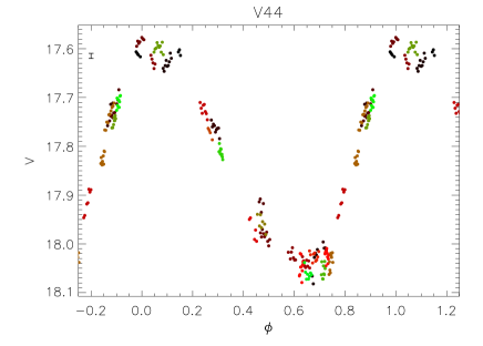
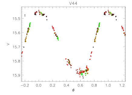
Figure 1: $V-$band light curves for V44 before (top) and after (bottom) self-calibration using the method of Bramich & Freudling (2012), showing significant improvement in light curve quality.

2.3.2 Photometric standards

We used secondary photometric standards in the FOV from Stetson (2000) covering the full range of colours of our CMD to convert the instrumental magnitudes we obtained from the pipeline reduction of the CCD images to standard Johnson-Kron-Cousins magnitudes. This was done by fitting a linear relation to the difference between the standard and instrumental magnitudes, and the instrumental $v-i$ colour of each photometric standard in our images. The resulting transformation relations are shown in Fig. 2. We compared our photometry with that of W94 by comparing mean magnitudes of RRL stars; this showed small differences of $<1\%$ in both $V$ and $I$ (see Table 3 in Sec. 3 for our mean magnitudes).

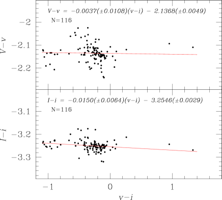
Figure 2: Relations used to convert from instrumental to standard Johnson-Kron-Cousins magnitudes for the $V$ (top) and $I$ (bottom) bands.

2.4 Astrometry

We derived astrometry for our CCD reference images by using Gaia to match $\sim 300$ stars manually with the UCAC3 catalogue (Zacharias et al. 2010). For the EMCCD reference, we derived the transformation by matching 10 stars to HST/ WFC3 images (e.g. Bellini et al. 2011). The coordinates we provide for all stars in this paper (Table 4) are taken from these astrometric fits. The rms of the fit residuals are 0.27 arcsec (0.57 pixel) for the CCD reference images and 0.09 arcsec (0.96 pixel) for the EMCCD reference.

3 Variables in M68

The first 28 (V1-V28) variables in this cluster were identified by H. Shapley and M. Ritchie (Shapley 1919, 1920), using fifteen photographs obtained with the 60-inch reflector telescope at Mt Wilson Observatory. All of these are RRL stars, except for V27, which was identified in the 1920 paper as a long-period variable; Greenstein et al. (1947) used a spectrum of V27 taken at the McDonald Observatory in 1939 to work out its radial velocity, and compared this to the cluster’s radial velocity to conclude that V27 is a long-period foreground variable star. Rosino & Pietra (1954) then used observations taken between 1951 and 1953 at Lojano Observatory to derive periods for 20 variables, and discovered three additional RRL stars (V29-V31). They also noted some irregularities in V3, V4, V29 and V30, whereby they could not derive precise periods for those four stars. van Agt & Oosterhoff (1959) found 7 more variables (V32-V38) analysing observations taken in 1950 with the Radcliffe 74-inch reflector telescope in South Africa. They also noticed many discrepancies between their derived periods and those published a few years earlier by Rosino & Pietra (1954), as well as differences in light curve morphologies. Terzan et al. (1973) announced another four variables in M68 (V39-V42), including the first SX Phe star in this cluster. Clement (1990) and C93 then studied 30 of the RRL stars, identifying 9 double-mode pulsators and detecting period changes since the earlier studies. Brocato et al. (1994) carried out the first CCD-era study of this cluster using the 1.5m ESO Danish Telescope, and soon after, W94 used CCD observations made in 1993 at the CTIO 0.9m telescope in Chile to discover an additional six variables (V43-V48), including another SX Phe star. Finally, Sariya et al. (2014) recently used observations from 2011 at the Sampurnanand telescope in Nainital, Northern India, to claim 9 new variable detections, including 5 RR1 stars, bringing the total number of published variables in this cluster to 57.

3.1 Detection of variables

3.1.1 CCD observations

We searched for variables using two methods: firstly we inspected the difference images visually and checked light curves of any objects that had residuals on a significant number of images. This did not enable us to detect any new variables. We also constructed an image from the sum of the absolute values of all difference images and inspected light curves at pixel positions with significant peaks on this stacked image; as with the first method, this method recovered most known variables, but did not enable us to detect new variables. Finally, we also conducted a period search, for periods ranging from 0.02 to 2 days, on all light curves using the “string length” method (e.g. Dworetsky 1983), and computed the ratio $S_{R}$ of the string length for the best-fit period to that for the worst (i.e. the string length for phasing with a random period). For light curves without periodic variations, $S_{R}$ is expected to be close to 1, although in practice, due to light curve scatter, the mean value is around 0.75; for true periodic light curves, $S_{R}\ll 1$. The distribution of $S_{R}$ is shown in Fig. 3. We inspected all light curves that fell below an arbitrary threshold of $S_{R}=0.5$, chosen by visually inspecting light curves sorted with ascending $S_{R}$.

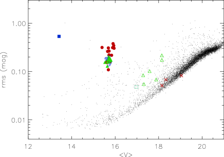
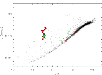
Figure 4: Root mean square magnitude deviation versus mean magnitude for all stars for which photometry was obtained. Plots are for the $V-$band (top) and $I-$band (bottom). Classified variables are marked with red filled circles (RR0), green filled triangles (RR1) and blue open inverted triangles (RR01), green open triangles (SX Phe), a blue square (for V27, the field Mira variable FI Hya), and a green open square (variable V53, of unknown type). Non-variable objects previously catalogued as variable in the literature are marked with red crosses.

Using this method, we recovered all known variables except for V32, which is outside our field of view; we were also able to derive periods for all of them, except for V27, which is now known to be a foreground variable star with a period of $\sim 322$ d (Pojmanski 2002); for V27 we also do not have an $I-$band light curve because it is saturated in our reference image. We also discovered four new variables, all of them SX Phe stars. Furthermore, we find that V40-42 are not variable within the limits of the rms in our data, given in Table 5, in agreement with the findings of W94. We also find that none of the new variables recently claimed by Sariya et al. (2014) is variable within the rms scatter of our data (Table 5, see also Fig. 4), and we therefore continue the variable numbering system from its standing prior to the publication of their paper.

We also confirm that many of the RRL stars are double-mode variables, as previously reported by Clement (1990) and C93, and we determine pulsation periods for both modes, when possible. Double-mode RRL stars in this cluster are discussed in Sec. 5.1.

In order to obtain the best possible period estimate for each star, we used archival data from previous studies of variability in this cluster by Rosino & Pietra (1953), Rosino & Pietra (1954), C93, W94, and Brocato et al. (1994). This gives us a baseline of up to 62 years for stars which were observed by Rosino & Pietra (1953), and of over 20 years for the stars that were observed in the 1993-1994 studies. The data of Rosino & Pietra (1953), Rosino & Pietra (1954), and Brocato et al. (1994) were previously not available in electronic format, and we have uploaded the light curves to the CDS for interested readers. For some of the stars, it was not possible to phase-fold the data sets without also fitting for a linear period change; for some even this did not lead to well-phased data sets, suggesting that some other effect is at work, such as a non-linear period change. Those are discussed in Sec. 3.3.

We also performed frequency analysis on all of the light curves in order to characterise the Blazhko effect (Blažko 1907), which can cause scatter in the phased light curve due to modulation of amplitude, frequency, phase, or a combination of those. We discuss the results of this search in Sec. 3.3.

Finally, we inspected the light curve of the standard star S28, which W94 found to be variable with an amplitude of $\sim 0.1$ mag. Our data show an increase in brightness of $\sim 0.1$ mag as well over the time span of our observations, confirming the variable nature of this star; we therefore assign it the variable number V53. Interestingly, however, we do not find significant variation in the $I-$band light curve of this star.

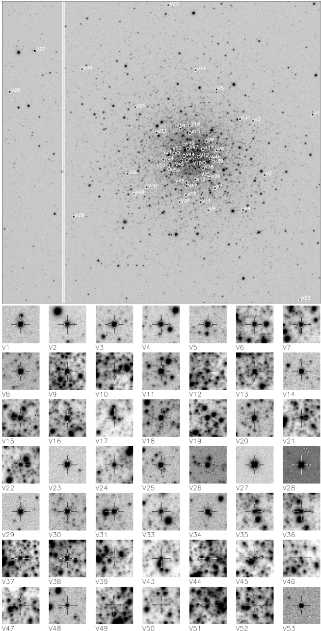
Figure 10: Finding chart for the confirmed variable objects in M68, using our $V$ reference image. North is up and East is to the left. The image size is 8.8 $\times$ 12.26 arcminutes, with each stamp 27.6^′′ $\times$ 27.6^′′. A white circle is centred on each variable and labelled with the variable number. The display scale has been modified where necessary to make the source as clear as possible on the stamps, and the location of the variable is also marked with a cross-hair. Stamps from the EMCCD reference image for V12, V44, V45 and V51 are shown in Fig. 12.

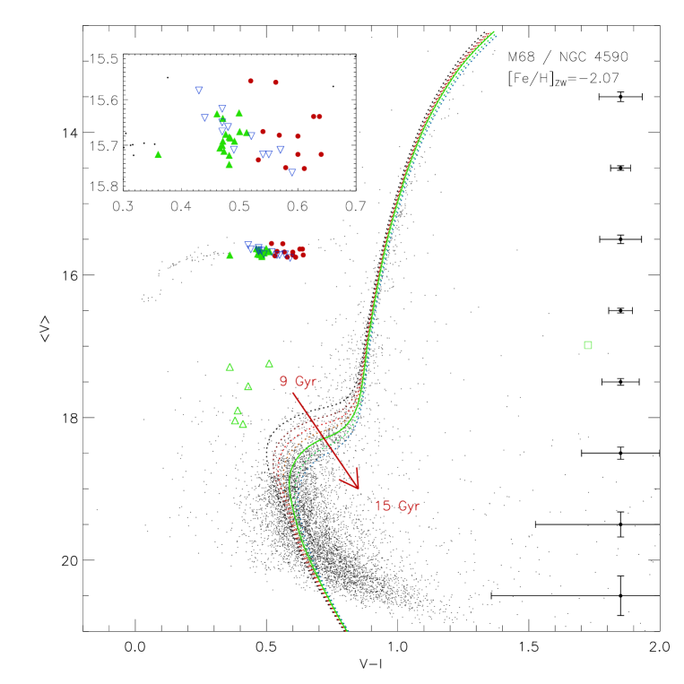
Figure 11: $(V-I),V$ colour-magnitude diagram from our photometry. The location of RR0 (red filled circles), RR1 (green filled triangles), RR01 (blue inverted triangles) and SX Phe (open green triangles) stars are shown. The variable V53 (unknown type) is shown as an open green square. Typical error bars are shown for different magnitude levels on the right-hand side of the plot. An inset in the top left corner of the plot shows a zoom of the instability strip region of the HB. For added information, isochrones for 9, 10, 11, 12, 13, 14 and 15 Gyr from Dotter et al. (2008) are overplotted in different colours; the best-fit isochrone (13 Gyr) is plotted as a thick green solid line.

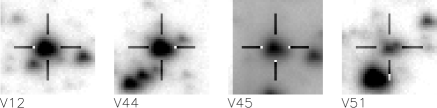
Figure 12: Stamps from the EMCCD reference image, for the stars within our EMCCD field of view, except V47, which is too close to the edge of the image. North is up and East is to the left. Each stamp is 3.6^′′ $\times$ 3.6^′′ and a cross-hair marks the location of the variable star.

$V-$band light curves for all of the variables objects are plotted on Figs. 5$-$9. $I-$band light curves are available for download with the electronic version of this article. A finding chart for all confirmed variables in M68 is shown in Fig. 10 and a CMD in Fig. 11. The CMD confirms the classification of the confirmed variables, with RRL located on the instability strip and SX Phe stars in the blue straggler region. We also show stamps of variables detected on our EMCCD images on Fig. 12.

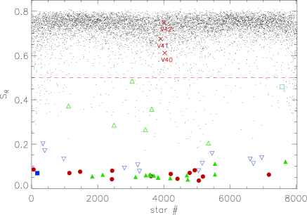
Figure 3: Plot of the distribution of the $S_{R}$ statistic as defined in the text, for our $V$-band light curves. A dashed line marks the threshold below which we searched for periodic variables. RR0, RR1 and RR01 variables are shown as red filled circles, green filled triangles and blue open inverted triangles respectively, SX Phe as open green triangles, the field Mira variable V27 (FI Hya) as a filled blue square, and the variable of unknown type V53 as an open green square. The three marked stars above the threshold are V40-V42, which we found to be non-variable.

#	Epoch	$P$	$\beta$	$\langle V\rangle$	$\langle I\rangle$	$A_{V}$	$A_{I}$	Type
	(HJD-2450000)	(d)	[$d{\rm Myr}^{-1}$]	[mag]	[mag]	[mag]	[mag]
RR0
V2	6411.5879	0.5781755	$-0.125$	15.75	15.17	0.72	0.49	RR0
V9	6412.5455	0.579043	$-$	15.72	15.12	0.69	0.40	RR0$b$
V10	6363.7134	0.551920	$-$	15.71	$-$	1.08	$-$	RR0$b$
V12	6369.4311	0.615546	$-$	15.56	15.04	0.89	0.61	RR0
V14	6373.4455	0.5568499	+1.553	15.73	15.20	1.11	0.77	RR0
V17	6411.5835	0.668424	$-$	15.68	15.08	0.82	0.54	RR0($b$?)
V22	6373.4162	0.5634451	$-$	15.67	15.13	1.15	0.75	RR0
V23	6410.5710	0.6588921	$-$	15.68	15.11	1.11	0.58	RR0
V25	6411.5323	0.6414842	$-0.488$	15.72	15.08	0.79	0.45	RR0$b$
V28	6363.7134	0.6067796	$+0.102$	15.75	15.14	1.18	0.70	RR0
V30	6370.5680	0.7336375	$+0.044$	15.64	15.00	0.37	0.25	RR0
V32	$-$	0.5882	$-$	$-$	$-$	$-$	$-$	RR0
V35	6381.6690	0.7025348	$-$	15.56	15.00	1.05	0.66	RR0
V46	6363.7743	0.7382510	$-$	15.64	15.01	0.54	0.37	RR0
RR1
V1	6381.7111	0.3495912	+0.273	15.70	15.23	$\sim$0.45	0.40	RR1
V5	6366.6697	0.2821009	$-0.497$	15.72	15.36	0.45	0.28	RR1$b$
V6	6385.6186	0.3684935	$-0.088$	15.69	15.20	0.53	0.34	RR1
V11	6370.6253	0.3649338	$+0.225$	15.71	15.24	$\sim$0.55	0.37	RR1
V13	6411.5829	0.3617370	$+0.116$	15.74	15.26	0.58	0.36	RR1
V15	6385.6092	0.3722615	$-$	15.68	15.20	0.53	0.34	RR1
V16	6381.6814	0.3819671	+0.066	15.69	15.22	0.50	0.35	RR1
V18	6363.7943	0.3673459	$-0.051$	15.72	15.24	0.55	0.37	RR1
V20	6363.7643	0.3857892	+0.234	15.68	15.20	0.56	0.34	RR1
V24	6370.4698	0.3764448	$-1.081$	15.68	15.20	0.50	0.34	RR1
V33	6385.5693	0.3905647	$-$	15.67	15.17	0.47	0.23	RR1
V37	6363.7727	0.3846092	$-$	15.64	15.17	0.47	0.33	RR1
V38	6370.4420	0.3828116	$-$	15.63	15.17	0.53	0.33	RR1
V43	6363.7527	0.3706144	$-$	15.71	15.24	0.57	0.35	RR1
V44	6371.4311	0.3850912	$-$	15.67	15.16	0.48	0.29	RR1
V47	6385.6436	0.3729255	$-$	15.63	15.13	0.49	0.32	RR1
RR01
V3	6381.6890	0.3907346	$-$	15.64	15.20	0.68	0.42	RR01
V4	6410.6485	0.3962175	$-$	15.67	15.20	0.61	0.40	RR01
V7	6381.7511	0.3879608	$-$	15.71	15.22	0.62	0.41	RR01
V8	6412.5861	0.3904076	$-$	15.65	15.18	0.53	0.34	RR01
V19	6368.6564	0.3916309	$-$	15.66	15.18	0.56	0.34	RR01
V21	6385.6233	0.4071121	$-$	15.62	15.15	0.64	0.42	RR01
V26	6369.4571	0.4070332	$-$	15.72	15.18	0.80	0.50	RR01
V29	6387.5498	0.3952413	$-$	15.71	15.14	0.56	0.30	RR01
V31	6385.6217	0.3996599	$-$	15.58	15.15	0.66	0.43	RR01
V34	6363.7673	0.4001371	$-$	15.76	15.17	$\sim$0.60	0.45	RR01
V36	6384.6470	0.415346	$-$	15.68	15.16	0.64	0.40	RR01
V45	6366.6760	0.3908187	$-$	15.72	15.17	0.52	0.30	RR01
SX Phe
V39	6433.2863	0.0640464	$-$	18.04	17.66	0.85	0.64	SX
V48	6387.6218	0.043225	$-$	17.29	16.93	0.24	$\sim$0.11	SX
V49	6387.6120	0.048469	$-$	18.09	17.68	0.59	0.40	SX
V50	6370.4561	0.065820	$-$	17.56	17.13	0.70	0.30	SXd
V51	6383.6232	0.058925	$-$	17.24	16.73	0.35	0.20	SX
V52	6410.5871	0.037056	$-$	17.90	17.51	0.25	$\sim$0.20	SX
Others
V27	2697.3	322.2342	$-$	9.8	$-$	4.03	$-$	Field Mira†
V53	$-$	$-$	$-$	16.98	15.26	$\geq 0.1$	$-$	?

Table 3: Epochs, periods, mean magnitudes and amplitudes $A$ in $V$ and $I$ for all confirmed variable stars in M68. V49, V50, V51 and V52 are newly discovered variables. A $b$ at the end of the variable type denotes stars which exhibit Blazhko modulation in their light curve. “SX” denotes SX Phe stars, and an appended “d” denotes double-mode pulsation. $\langle V\rangle$ and $\langle I\rangle$ are intensity-weighted mean magnitudes. Note that those are calculated from Fourier fits for all RRL stars, as the mean magnitude is stable even for unsatisfactory fits. For stars without good Fourier fits, amplitudes are calculated from the data. For V27, the data are taken from the ASAS catalogue Pojmanski (2002). The data for V32 are taken from C93, as that star is outside of our field of view. Values of the period-change rate parameter $\beta$ are also given, where relevant (see Sec. 3.2); in those cases, the value of $P$ given corresponds to the instantaneous period at the epoch. ^†this star is FI Hydra.

#	RA	DEC
RR0
V2	12:39:15.29	-26:45:24.6
V9	12:39:25.57	-26:44:00.8
V10	12:39:25.96	-26:44:54.7
V12	12:39:26.918	-26:44:39.73
V14	12:39:27.54	-26:41:04.2
V17	12:39:29.02	-26:45:52.4
V22	12:39:32.30	-26:45:01.6
V23	12:39:32.41	-26:38:23.0
V25	12:39:38.15	-26:42:37.2
V28	12:40:00.31	-26:41:59.8
V30	12:39:36.07	-26:45:55.6
V32	12:39:03.29	-26:55:18.0
V35	12:39:25.19	-26:45:32.5
V46	12:39:24.84	-26:44:43.4
RR1
V1	12:39:06.86	-26:42:53.3
V5	12:39:23.83	-26:41:52.3
V6	12:39:23.77	-26:44:23.6
V11	12:39:26.56	-26:46:32.7
V13	12:39:27.49	-26:45:35.9
V15	12:39:28.50	-26:43:40.9
V16	12:39:28.54	-26:43:22.1
V18	12:39:29.12	-26:46:15.2
V20	12:39:30.26	-26:46:33.2
V24	12:39:33.15	-26:44:46.6
V33	12:39:34.41	-26:43:40.7
V37	12:39:26.18	-26:44:20.9
V38	12:39:26.09	-26:45:08.3
V43	12:39:29.06	-26:45:43.7
V44	12:39:29.477	-26:44:38.06
V47	12:39:28.831	-26:44:19.92
RR01
V3	12:39:17.33	-26:43:09.9
V4	12:39:19.06	-26:46:51.3
V7	12:39:24.02	-26:45:57.7
V8	12:39:25.18	-26:46:52.5
V19	12:39:30.15	-26:43:30.4
V21	12:39:31.19	-26:44:32.0
V26	12:39:39.46	-26:45:22.9
V29	12:39:48.93	-26:47:10.1
V31	12:39:19.65	-26:43:05.4
V34	12:39:47.56	-26:41:03.5
V36	12:39:24.89	-26:45:32.1
V45	12:39:29.989	-26:44:49.18
SX Phe
V39	12:39:24.34	-26:44:51.8
V48	12:39:38.27	-26:46:12.4
V49	12:39:29.52	-26:44:09.3
V50	12:39:32.12	-26:45:10.5
V51	12:39:28.986	-26:44:48.47
V52	12:39:30.57	-26:44:30.1
Others
V27	12:39:55.92	-26:40:17.4
V53	12:39:08.91	-26:50:33.8

Table 4: Equatorial celestial coordinates of all confirmed variables in M68 at the epoch of the reference image, HJD$\sim 2456385.6$ d. More precise coordinates are given for stars which are within the field of view of the EMCCD reference image, with epoch $\sim 2456451$ d. The coordinates for V32, which is outside of our field of view, are from C93.

#	$\langle V\rangle$	rms ($V$)	$\langle I\rangle$	rms ($I$)
#	[mag]	[mag]	[mag]	[mag]
V40	18.32	0.068	17.50	0.075
V41	18.15	0.052	17.36	0.060
V42	19.05	0.083	18.36	0.156
SV49	14.72	0.008	13.67	0.007
SV50	15.15	0.010	14.14	0.008
SV51	12.68	0.013	$-$	$-$
SV52	18.17	0.225	$-$	$-$
SV53	18.60	0.077	17.94	0.14
SV54	18.48	0.361	17.00	0.14
SV55	17.04	0.023	16.21	0.03
SV56	19.81	0.192	18.97	0.31
SV57	16.81	0.016	15.91	0.02

Table 5: Light curve mean magnitudes and rms values for V40-42, for which we do not find evidence of variability, as well as for the “new” variables published by Sariya et al. (2014). Since Sariya et al. (2014) assigned those variables new V numbers, we add an “S” as a prefix to avoid confusion with the confirmed variables in this paper. Note that the mean magnitudes of V41 and V42 are significantly different from those given by W94. For V41 we suggest that this might be due to blending by V16 in their data, but no explanation is offered for the difference with V42.

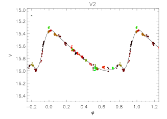
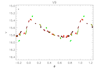
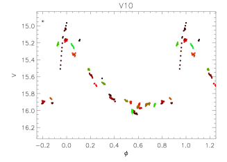
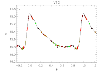
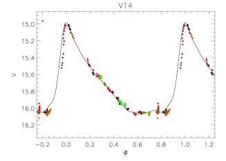
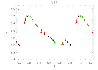
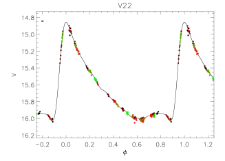
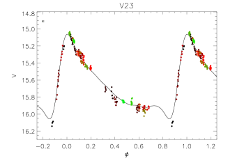
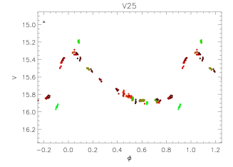
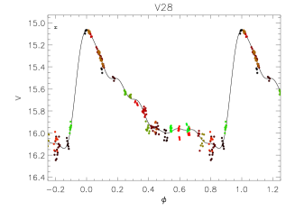
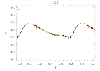
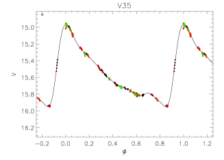
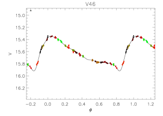
Figure 5: Phased $V$-band light curves of the confirmed RR0 variables in M68. Data from different nights are plotted in different colours (electronic version only), with a colour bar provided for reference (top panel). On the light curves for which a good Fourier decomposition could be obtained, the fit is overplotted. The size of typical 1-$\sigma$ error bars is plotted in the top left corner. The magnitude scale is the same on all plots in order to facilitate comparison of variation amplitude.

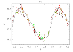
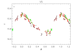
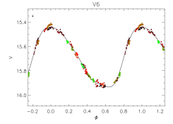
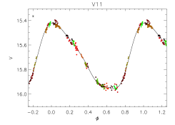
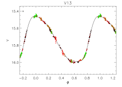
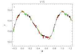
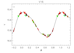
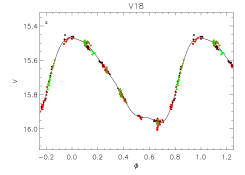
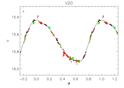
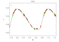
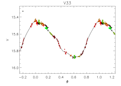
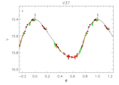
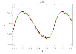
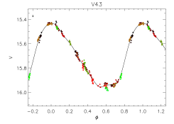
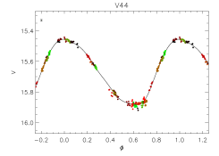
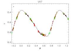
Figure 6: Same as Fig. 5, but for RR1 stars.

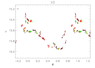
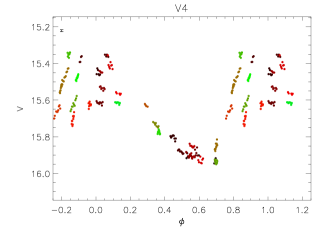
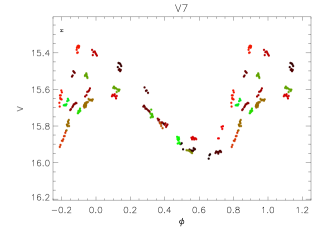
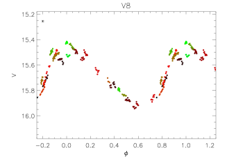
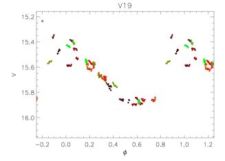
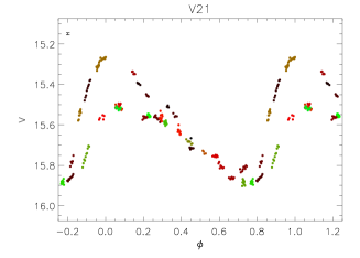
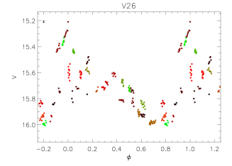
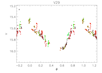
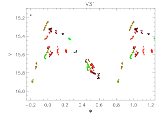
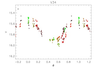
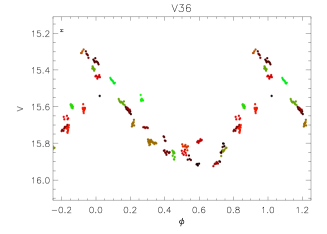
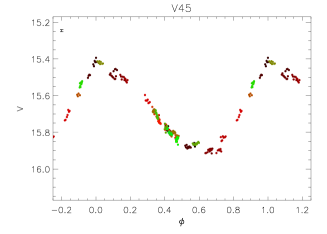
Figure 7: Phased $V-$band light curves of the RR01 stars. The light curves are phased with the first-overtone pulsation period. A typical 1-$\sigma$ error bar is plotted in the top left corner. The magnitude scale is the same on all plots in order to facilitate comparison of variation amplitude.

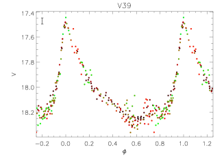
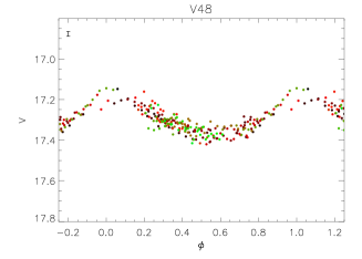
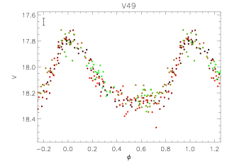
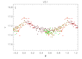
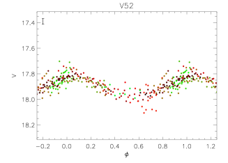
Figure 8: Phased $V-$band light curves of the confirmed SX Phe stars in M68, with a typical 1-$\sigma$ error bar plotted in the top left corner. The magnitude scale is the same on all plots in order to facilitate comparison of variation amplitude.

Figure 9: Unphased $V-$band light curves of the variables V27 (FI Hya) and V53 (unknown type), plotted with 1-$\sigma$ error bars.

3.1.2 EMCCD observations

We repeated the method we used for CCD observations to search for variability in the EMCCD observations we obtained. Of the known variables, only V44 has a light curve, with V12, V45 and V47 also located within our FOV, but being too close to the edge to allow for photometric measurements. Furthermore, the camera was changed in May 2013, with a slightly different filter after that, meaning that measurements from images taken before and after the change need to be treated as separate light curves.

We also detect the new variable V51, and confirm the period found with the CCD data for this object. The EMCCD light curves for V44 and V51 are shown in Fig. 13.

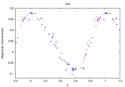
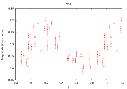
Figure 13: EMCCD light curve for variables V44 and V51. See Table 3 for information about these variables. Note that for V44 we show the light curves before (blue + signs) and after (red asterisks) the camera change as separate light curves, as discussed in the text. For V51, we show only the light curve after the change, as the photometry before was too poor.

3.2 Period changes in RRL stars

Period changes have been observed in many RRL stars, both in the Galactic field and in globular clusters. Period changes are usually classed as evolutionary or non-evolutionary. Evolutionary period changes of stars on the instability strip are understood to be due to their radius increasing and contracting. These only account for slowly increasing or decreasing changes, however, and in many RRL, abrupt period changes have been observed (e.g. Stagg & Wehlau 1980) which cannot be explained by such evolution. As yet, there is no clear explanation for such changes.

As noted by Jurcsik et al. (2012), in spite of this, period-change rates of RRL in a globular cluster can inform us about its general evolution using theoretical models. Lee et al. (1990) suggested that in Oosterhoff type II clusters, most of the RRL pass through the instability strip from blue to red when reaching the end of helium burning in their core. Since such a blue-to-red evolution would also lead to a period increase, Lee (1991) argued that a mean positive value of the period change rate $\beta$ in a cluster would support this scenario. Furthermore, Rathbun & Smith (1997) showed that the average period change should be smaller for Oosterhoff I clusters than Oosterhoff II. Few comprehensive studies of period changes in cluster RRL have been published; Smith & Wesselink (1977) derived period changes for RRL in the Oosterhoff type II cluster M15, with a mean of $\beta=0.11\pm 0.36\,{\rm d\,Myr}^{-1}$. For the Oosterhoff type I cluster M3, Jurcsik et al. (2012) found a slightly positive mean value of $\beta\sim 0.01\,{\rm d\,Myr}^{-1}$, agreeing with the theoretical predictions of Lee (1991) and the findings of Rathbun & Smith (1997).

The parameter $\beta$ is defined such that the period at time $t$ is given by

$$P(t)=P_{0}+\beta(t-E),$$ (1)

where $P_{0}$ is the period at the (arbitrary) epoch $E$, and $\beta$ as expressed in Eq. (1) is in units of $\mathrm{d\,d}^{-1}$; however $\beta$ is usually expressed in ${\rm d\,Myr}^{-1}$ as a more natural unit. The number of cycles $N_{E}$ elapsed at time $t$ since the epoch $E$ can then be calculated as

$$N_{E}=\int_{E}^{t}\frac{dx}{P(x)}=\frac{1}{\beta}\ln\left[1+\frac{\beta}{P_{0}}(t-E)\right]\,.$$ (2)

The phase is then

$$\phi=N_{E}-\lfloor N_{E}\rfloor\,.$$ (3)

Here we use data stretching back to 1951 (see Sec. 3) to derive period changes for RR0 and RR1 stars for which data sets are not well phased and/or aligned with a single constant period. To do this we performed a grid search in the ($P_{0},\beta$) plane by minimising the string length of our data combined with those of W94 (both taken in $V-$band); we then searched manually around the best-fit solution incorporating other data sets taken in different passbands. As a consistency check, we also calculated period-change parameters using the O-C method. This consists of using an ephemeris to predict the times of maxima in the light curves, and then plotting the difference between observed and predicted times of maxima against time. By fitting a quadratic function to this, a value of $\beta$ can be derived; two such fits are shown in Fig. 14 for variables V14 and V28, which produced values of $\beta$ consistent with the values derived using the grid method. The interested reader is referred to the papers of, e.g., Belserene (1964) and Nemec et al. (1985) for further details. We found here that the values we found for $\beta$ using the O-C method did not always produce well-phased light curves for all data sets. This is most likely due to the small number of observed maxima available for the variables in this cluster. For the cases where the two methods were not in agreement, we used the value found with the grid search. C93 derived period-change rates by computing periods for their light curves, and for archival light curves, and subtracting one from another. The method used here, and the availability of more data, mean that our period-change calculations should be more robust. The signs of our values of $\beta$ agree with those of C93 except for V2 and V18, which, however, had very large associated error bars in that study.

Figure 14: O-C plots for variables V14 and V28 showing the quadratic fit to the time-dependence of the difference between observed and predicted times of light curve maxima. The values found using this quadratic fit for V14 and V28 are consistent with those derived using our grid fitting method (see text), $\beta$=+1.553 d Myr^-1 (V14) and $\beta=$+0.102 d Myr^-1 (V28).

The values of $\beta$ from our analysis are listed in Table 3. Examples of phased light curves are shown in Fig. 15 for V14 and V18. The large spread in values found for $\beta$ means that we are unable to draw any firm conclusion about the general evolution of M68. We find a mean value of $\langle\beta\rangle=0.02\pm 0.57$ d Myr^-1.

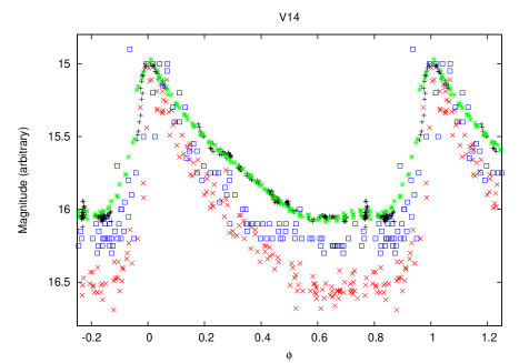
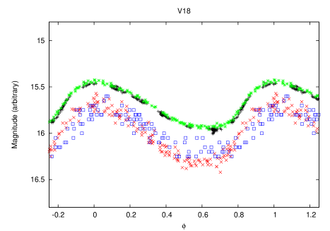
Figure 15: Phased light curves for V14 (top) and V18 (bottom), showing the data sets of this paper (black, + symbols), W94 (green asterisks), C93 (red crosses) and Rosino & Pietra (1954, blue squares). The light curves were phased using a period change of +1.553 d Myr^-1 (V14) and $-0.051$ d Myr^-1 (V18).

3.3 Discussion of individual RRL variables

Note that RR0 variables are plotted in Fig. 5, RR1 in Fig. 6, and RR01 in Fig. 7. Details of period-change calculations are given in Sec. 3.2.

• V1: We could only phase the different data sets by including a period-change parameter $\beta=0.273$ d Myr^-1.

• V2: W94 noted that this star features Blazhko modulation, but our light curves do not enable us to confirm this. We found that a negative period change parameter $\beta=-0.125$ d Myr^-1 was needed to phase-fold the various data sets.

• V5: This star requires a linear period change $\beta=-0.497$ d Myr^-1 to phase the different data sets; however, the data from C93 are not phased well with our best-fit period and period change parameter $\beta$; according to W94, this star also has slow amplitude variations with a period of several days; the scatter in our data is consistent with that assessment.

• V6: The data from Rosino & Pietra (1954) are not aligned with the other data sets with a constant period; we find a period-change parameter of $\beta=-0.088$ d Myr^-1. The light curve may suggest some Blazhko modulation, but our data do not allow us to make a strong claim about this.

• V9: Our light curve shows Blazhko modulation, as proposed by W94.

• V10: Our light curve for this object shows clear Blazhko amplitude modulation; interestingly, W94 found a constant amplitude but a variable period.

• V11: We could only phase the data sets simultaneously by including a period-change parameter $\beta=0.225$ d Myr^-1.

• V12: We find no evidence of Blazhko modulation for this star, contrary to W94, who found strong cycle-to-cycle variations; this may be due do the baseline of W94 being longer by $\sim 50$ days.

• V13: We find that the inclusion a period-change parameter is necessary to phase all the light curves; we find $\beta=0.116$ d Myr^-1

• V14: W94 noted a variation in shape for the bump at minimum brightness which we cannot confirm in our light curve. We also found that a rather large period change parameter $\beta=1.553$ d Myr^-1 was necessary to phase-fold all the data sets (see Fig. 15).

• V15: Our observations show some slight residual scatter, which might suggest Blazhko modulation; some evidence of similar scatter is visible in the data of W94.

• V16: A period-change parameter $\beta=0.066$ d Myr^-1 was included to improve the phase-folding of the various data sets.

• V17: We do not find evidence for the Blazhko effect in this star as suggested by W94 on the timescales covered by our baseline. However, comparison of our light curve with that of W94 (Fig. 16) shows clearly that the amplitude of the light curve is larger in our data set, which might indicate that modulation is present but slow.

• V18, V20, V24: These stars all required the inclusion of a period-change parameter for satisfactory phase-folding of available data sets.

• V25: We find a period-change parameter to phase all the data sets of $\beta=-0.488$ d Myr^-1. The light curve also shows Blazhko modulation, as was already noted by W94.

• V28: We tentatively suggest that this star might be affected by the Blazhko effect. A period change parameter of $\beta=0.102$ d Myr^-1 was found to improve the phase-folding of all data sets.

• V30: A small positive period-change parameter $\beta=0.044$ d Myr^-1 was found to be necessary to phase all data sets.

• V33: This star is now RR1, but used to be RR01, as first noted by C93. Like C93, we fail to detect signs of secondary pulsations which were visible in the data of van Agt & Oosterhoff (1959).

• V47: We do not confirm the suggestion of W94 of this star being affected by Blazhko modulation; this may be due to the longer baseline of the W94 data.

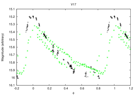
Figure 16: Phased light curves for V17, showing the $V-$band data sets of this paper (black, + symbols) and W94 (green asterisks). The amplitude is larger in our data by $\sim 0.15$ mag compared to the observations of W94,; we suggest that this might be due to slow amplitude modulation.

4 Fourier decomposition of RR Lyrae star light curves

We performed a Fourier decomposition of the $V-$band light curves of RRL variables in order to derive several of their properties with well-established empirical relations. We can then use individual stars’ properties to estimate the parameters of the host cluster. Fourier decomposition equates to fitting light curves with the Fourier series

$$m(t)=A_{0}+\sum_{k=1}^{N}A_{k}\cos\left[\frac{2\pi k}{P}(t-E)+\phi_{k}\right]\,,$$ (4)

where $m(t)$ is the magnitude at time $t$, $N$ is the number of harmonics used in the fit, $P$ is the period of the variable, $E$ is the epoch, and $A_{k}$ and $\phi_{k}$ are the amplitude and phase of the $k^{th}$ harmonic respectively. The epoch-independent Fourier parameters are then defined as

$$R_{ij} = A_{i}/A_{j}$$ (5)

$$\phi_{ij} = j\phi_{i}-i\phi_{j}\,.$$ (6)

In each case we used the lowest number of harmonics that provided a good fit, to avoid over-fitting variations in the light curves due to noise. We also checked the sensitivity of the parameters we derived to the number of harmonics $N$, and we used only light curves with stable parameters, i.e. ones that showed little variation with $N$, to estimate cluster parameters. Double-mode pulsators and objects exhibiting signs of Blazhko modulation are also excluded from the following analysis.

The $A_{k}$ coefficients for the first four harmonics and the Fourier parameters $\phi_{21},\phi_{31}$ and $\phi_{41}$ are given in Table 6 for the light curves for which we could obtain a Fourier decomposition. We used the deviation parameter $D_{m}$, defined by Jurcsik & Kovács (1996), as an estimate of the reliability of derived parameters, and use $D_{m}<5$ (e.g. Cacciari et al. 2005) as a selection criterion. The value of $D_{m}$ for each of the successful Fourier decompositions is given in Table 6.

We did not fit RR0 stars V9, V10, and V25, and RR1 star V5, because they all exhibit Blazhko-type modulation. Furthermore, we did not use the fits of V14, V28, V30 and V46 to derive star properties because those fits have a value of $D_{m}>5$. V17 was not fitted either because the parameters varied significantly with the number of harmonics used in the fit, as well as showing signs of slow amplitude modulation (see Sec. 3.3). This leaves us with 5 RR0 and 15 RR1 stars for which we derive individual properties in the next section. We also note that for V1, V2, V14, V23, and V30, we combined our data with that of W94 in order to derive fits, due to insufficient phase coverage of our data alone.

#	$A_{0}$	$A_{1}$	$A_{2}$	$A_{3}$	$A_{4}$	$\phi_{21}$	$\phi_{31}$	$\phi_{41}$	$N$	$D_{m}$
RR0
V2	15.749(2)	0.281(2)	0.086(2)	0.057(2)	0.042(2)	4.031(17)	8.039(23)	6.073(32)	9	4.34
V12	15.559(2)	0.325(2)	0.145(2)	0.113(2)	0.075(2)	3.870(10)	7.940(12)	5.774(19)	11	3.11
V14	15.732(2)	0.421(2)	0.154(3)	0.116(3)	0.068(3)	3.926(13)	7.926(18)	5.765(27)	10	5.04
V22	15.670(2)	0.424(2)	0.179(2)	0.136(2)	0.100(2)	3.836(9)	7.780(13)	5.717(18)	11	2.36
V23	15.678(3)	0.338(3)	0.159(3)	0.118(3)	0.078(3)	3.899(20)	8.157(28)	6.163(40)	8	1.83
V28	15.751(2)	0.371(2)	0.178(2)	0.146(2)	0.076(2)	3.842(8)	8.363(11)	6.064(17)	8	6.44
V30	15.637(2)	0.165(2)	0.059(2)	0.029(2)	0.011(2)	4.121(24)	8.510(43)	7.114(104)	7	17.59
V35	15.562(2)	0.338(2)	0.163(2)	0.113(2)	0.081(2)	4.041(8)	8.411(11)	6.478(14)	9	2.87
V46	15.637(2)	0.209(2)	0.091(2)	0.055(2)	0.026(3)	4.090(25)	8.684(35)	7.187(47)	10	7.94
RR1
V1	15.700(2)	0.296(3)	0.059(3)	0.023(3)	0.016(3)	4.558(39)	2.581(93)	1.461(125)	4	$-$
V6	15.691(1)	0.251(1)	0.040(2)	0.021(1)	0.009(1)	4.619(15)	2.962(31)	2.102(73)	4	$-$
V11	15.706(1)	0.265(2)	0.052(2)	0.025(2)	0.007(2)	4.554(13)	2.521(25)	1.837(78)	4
V13	15.742(1)	0.274(2)	0.049(2)	0.028(2)	0.013(2)	4.536(15)	2.722(23)	1.066(47)	5	$-$
V15	15.684(1)	0.241(1)	0.041(2)	0.019(2)	0.007(2)	4.636(15)	3.074(29)	1.883(73)	5	$-$
V16	15.691(1)	0.229(2)	0.039(2)	0.023(2)	0.001(2)	4.706(16)	2.865(31)	1.936(410)	6	$-$
V18	15.722(1)	0.249(2)	0.046(2)	0.027(2)	0.015(2)	4.566(15)	2.873(24)	1.930(48)	4	$-$
V20	15.676(1)	0.239(1)	0.036(1)	0.019(2)	0.004(1)	4.806(15)	3.129(27)	2.355(126)	5	$-$
V24	15.682(2)	0.247(2)	0.048(2)	0.022(2)	0.011(2)	4.637(17)	2.894(35)	1.978(68)	6	$-$
V33	15.670(1)	0.211(2)	0.030(2)	0.013(2)	0.006(2)	4.627(23)	2.983(51)	2.787(115)	6	$-$
V37	15.641(1)	0.227(2)	0.036(2)	0.011(2)	0.006(2)	4.392(21)	3.013(59)	2.440(98)	4	$-$
V38	15.631(1)	0.250(2)	0.038(2)	0.016(2)	0.006(2)	4.537(16)	3.180(37)	2.052(93)	4	$-$
V43	15.713(1)	0.261(2)	0.048(2)	0.021(2)	0.011(2)	4.439(17)	2.408(35)	1.378(62)	5	$-$
V44	15.672(2)	0.216(2)	0.032(2)	0.012(2)	0.004(2)	4.706(31)	3.205(62)	1.854(147)	5	$-$
V47	15.629(2)	0.248(2)	0.048(2)	0.016(2)	0.007(2)	4.645(21)	2.799(62)	2.676(123)	5	$-$

Table 6: Parameters from the Fourier decomposition. Numbers in parentheses are the 1-$\sigma$ uncertainties on the last decimal place.

#	$\mathrm{[Fe/H]_{ZW}}$	$\mathrm{[Fe/H]_{UVES}}$	$M_{V}$	$\log(L/L_{\bigodot})$	$\log T_{\mathrm{eff}}$
RR0
V2	-1.85(2)	-2.17(6)	0.578(30)	1.679(12)	3.804(2)
V12	-2.09(1)	-2.81(3)	0.522(24)	1.704(10)	3.800(2)
V22	-2.04(1)	-2.72(4)	0.498(27)	1.709(11)	3.807(2)
V23	-2.04(3)	-2.58(8)	0.455(27)	1.733(11)	3.797(2)
V35	-1.97(1)	-2.21(3)	0.399(30)	1.758(12)	3.795(2)
RR1
V1	-2.06(3)	$-$	0.521(23)	1.658(10)	3.855(2)
V6	-2.06(2)	$-$	0.533(21)	1.655(9)	3.854(1)
V11	-2.12(1)	$-$	0.548(21)	1.650(9)	3.852(1)
V13	-2.08(1)	$-$	0.524(21)	1.658(9)	3.854(1)
V15	-2.05(2)	$-$	0.538(21)	1.653(9)	3.854(1)
V16	-2.11(1)	$-$	0.550(21)	1.650(9)	3.851(1)
V18	-2.07(1)	$-$	0.511(21)	1.664(9)	3.854(1)
V20	-2.08(1)	$-$	0.529(21)	1.658(9)	3.852(1)
V24	-2.10(2)	$-$	0.517(21)	1.663(9)	3.852(1)
V33	-2.11(2)	$-$	0.526(21)	1.661(9)	3.851(1)
V37	-2.10(2)	$-$	0.540(21)	1.654(9)	3.852(1)
V38	-2.06(2)	$-$	0.536(21)	1.655(9)	3.853(1)
V43	-2.14(1)	$-$	0.531(21)	1.658(9)	3.851(1)
V44	-2.07(2)	$-$	0.533(21)	1.656(9)	3.853(1)
V47	-2.10(2)	$-$	0.536(21)	1.655(9)	3.852(1)

Table 7: Physical parameters for the RRL variables calculated using the Fourier decomposition parameters and the relations given in the text. Numbers in parentheses are the 1-$\sigma$ uncertainties on the last decimal place. The values of $\mathrm{[Fe/H]_{UVES}}$ listed in this table for RR0 stars are derived using the relation of Nemec et al. (2013). In addition, we note that Smith & Manduca (1983) found $\mathrm{[Fe/H]_{ZW}}\approx-2.15$ for V2 and $\mathrm{[Fe/H]_{ZW}}\approx-2.07$ for V25, using the $\Delta$S method (see Sec. 4.1). Note that errors quoted for $\log T_{\mathrm{eff}}$ are statistical only and not systematic; we could not calculate systematic errors for $\log T_{\mathrm{eff}}$ as no errors are given on the empirical coefficients in Eqs. (4.2) and (16). Errors on $M_{V}$ and $\log(L/L_{\bigodot})$ for RR1 stars are dominated by the error on the zero-point $K_{0}$ in Eq. (18).

4.1 Metallicity

In this section we derive metallicities for each variable for which a good Fourier decomposition, according to our selection criteria discussed above, could be obtained. To do this, we use empirical relations from the literature. For RR0 stars, we used the relation of Jurcsik & Kovács (1996), which expresses [Fe/H] as a function of the period and of the Fourier parameter $\phi^{s}_{31}$; the $s$ superscript denotes that Jurcsik & Kovács (1996) derived their relations using sine series, whereas we fit cosine Fourier series (Eq. 4). The Fourier parameters can be easily converted using the equation

$$\phi^{s}_{ij}=\phi_{ij}-(i-j)\,\frac{\pi}{2}\,.$$ (7)

[Fe/H] can then be expressed as

$$\mathrm{[Fe/H]_{J}}=-5.038-5.394\,P+1.345\,\phi^{s}_{31}\,,$$ (8)

where the subscript J denotes a non-calibrated metallicity, and the period $P$ is in days. This value can be transformed to the metallicity scale of Zinn & West (1984) (hereafter ZW) via the simple relation from Jurcsik (1995),

$$\mathrm{[Fe/H]_{ZW}}=\frac{\rm[Fe/H]_{J}-0.88}{1.431}\,.$$ (9)

Kovács (2002) investigated the validity of this relation, and found that Eq. (8) yields metallicity values that are too large by $\sim 0.2$ dex for metal-poor clusters. This was supported by the findings of Gratton et al. (2004) and Di Fabrizio et al. (2005), who compared metallicity values for RRL stars in the Large Magellanic Cloud (LMC) using both spectroscopy and Fourier decomposition. Therefore we include a shift of -0.20 dex (on the $\mathrm{[Fe/H]_{J}}$ scale) or -0.14 dex (on the ZW scale) to the metallicity values derived for RR0 stars using Eq. (8).

More recently, Nemec et al. (2013) derived a relation for the metallicity of RR0 stars, using observations of RRL taken with the Kepler space telescope,

$$\mathrm{[Fe/H]_{UVES}}=b_{0}+b_{1}P+b_{2}\phi^{s}_{31}+b_{3}\phi^{s}_{31}P+b_{4}\left(\phi^{s}_{31}\right)^{2}\,,$$ (10)

where $\mathrm{[Fe/H]_{UVES}}$ is the metallicity on the widely-used scale of Carretta et al. (2009a), and the constant coefficients were determined by Nemec et al. (2013) as $b_{0}=-8.65\pm 4.64$, $b_{1}=-40.12\pm 5.18$, $b_{3}=6.27\pm 0.96$ and $b_{4}=-0.72\pm-0.72\pm 0.17$. The scale of Carretta et al. (2009a) was derived using spectra of red giant branch (RGB) stars obtained using GIRAFFE and UVES. ZW metallicity values can be transformed to that scale (hereafter referred to as the UVES scale) using

$$\mathrm{[Fe/H]_{UVES}}=-0.413+0.130\,\mathrm{[Fe/H]_{ZW}}-0.356\,\mathrm{[Fe/H]_{ZW}}^{2}\,.$$ (11)

In the discussion that follows, we considered RR0 metallicity values obtained both with the scale of Jurcsik & Kovács (1996) and that of Nemec et al. (2013).

For the RR1 variables, we used the relation of Morgan et al. (2007) to derive metallicity values; this relates [Fe/H], $P$ and $\phi_{31}$ as

$$\mathrm{[Fe/H]_{ZW}} = 2.424-30.075\,P+52.466\,P^{2}$$

$$+0.982\,\phi_{31}+0.131\phi_{31}^{2}-4.198\,\phi_{31}P\,.$$

Metallicity values calculated using Eqs. (8) & (9) and (4.1) are listed in Table 7.

We note that the metallicities of only two RRL stars in M68 have previously been measured in the literature. Smith & Manduca (1983) measured the spectroscopic metallicity index $\Delta S$ for the RR0-type variables V2 and V25 as 11.0 and 10.5, respectively, which yield metallicities $\mathrm{[Fe/H]_{ZW}}\approx-2.15$ and $-2.07$, respectively, when converted to the ZW scale via the following relation from Suntzeff et al. (1991):

$$\mathrm{[Fe/H]_{ZW}}=-0.158\Delta{\rm S}-0.408\,.$$ (13)

We include these metallicity measurements as a footnote to Table 7 for the sake of completeness.

4.2 Effective Temperature

Jurcsik (1998) derived empirical relations to calculate the effective temperature of fundamental-mode RRL stars, relating the $(V-K)_{0}$ colour to $P$ and to several of the Fourier coefficients and parameters:

$$(V-K)_{0} = 1.585+1.257\,P-0.273\,A_{1}-0.234\,\phi^{s}_{31}$$

$$+0.062\,\phi^{s}_{41}$$

$$\log\,T_{\mathrm{eff}} = 3.9291-0.1112\,(V-K)_{0}$$

$$-0.0032\,\mathrm{[Fe/H]_{J}}\,.$$

Simon & Clement (1993) used theoretical model to derive a corresponding relation for RR1 stars,

$$\log\,T_{\mathrm{eff}}=3.7746-0.1452\log\,P+0.0056\,\phi_{31}\,.$$ (16)

We use those relations to derive $\log T_{\mathrm{eff}}$ for all of our RR0 and RR1 stars, and give the resulting values in Table 7. As we mentioned in previous analyses (e.g. Arellano Ferro et al. 2008), there are some important caveats to consider when estimating temperatures with Eqs. (4.2) and (16). The values of $\log T_{\mathrm{eff}}$ for RR0 and RR1 stars are on different absolute scales (e.g. Cacciari et al. 2005), and temperatures derived using these relations show systematic deviations from those predicted by Castelli (1999) in their evolutionary models, or by the temperature scales of Sekiguchi & Fukugita (2000). However, we use these in order to have a comparable approach to that taken in our previous studies of clusters.

4.3 Absolute Magnitude

We use the empirical relations of Kovács & Walker (2001) to derive $V$-band absolute magnitudes for the RR0 variables,

$$M_{V}=-1.876\log P-1.158\,A_{1}+0.821\,A_{3}+K_{0}\,,$$ (17)

where $K_{0}$ is the zero-point of the relation. Using the absolute magnitude of the star RR Lyrae of $M_{V}=0.61\pm 0.10$ mag derived by Benedict et al. (2002), and a Fourier decomposition of its light curve, Kinman (2002) determined a zero-point for Eq. (17) of $K_{0}=0.43$ mag. Here, however we adopt a slightly different value of $K_{0}=0.41\pm 0.02$ mag, as in several of our previous studies (e.g. Arellano Ferro et al. 2010), in order to maintain consistency with a true distance modulus of $\mu_{0}=18.5$ mag for the LMC (Freedman et al. 2001). A nominal error of 0.02 mag on $K_{0}$ was adopted in the absence of uncertainties on $K_{0}$ in the literature.

For RR1 variables, we use the relation of Kovács (1998),

$$M_{V}=-0.961\,P-0.044\,\phi^{s}_{21}-4.447\,A_{4}+K_{1}\,,$$ (18)

where we adopted the zero-point value of $K_{1}=1.061\pm 0.020$ mag (Cacciari et al. 2005), with the same justification as for our choice of $K_{0}$.

We also converted the magnitudes we obtained to luminosities using

$$\log\left(L/L_{\bigodot}\right)=-0.4\,\left[M_{V}+B_{C}(T_{\mathrm{eff}})-M_{\rm bol,\bigodot}\right]\,,$$ (19)

where $M_{\rm bol,\bigodot}$ is the bolometric magnitude of the Sun, $M_{\rm bol,\bigodot}=4.75$ mag, and $B_{C}(T_{\mathrm{eff}})$ is a bolometric correction which we estimate by interpolating from the values of Montegriffo et al. (1998) for metal-poor stars, and using the value of $\log T_{\mathrm{eff}}$ we derived in the previous section. Values of $M_{V}$ and $\log(L/L_{\bigodot})$ for the RR0 and RR1 variables are listed in Table 7. Using our average values of $M_{V}$, in conjunction with the average values of $\mathrm{[Fe/H]_{ZW}}$ (Sec. 4.1), we find a good agreement with the $M_{V}-\mathrm{[Fe/H]_{ZW}}$ relation derived in the literature (e.g. Kains et al. 2012, see Fig. 9 of that paper).

4.4 Masses

Empirical relations also exist to derive masses of RRL stars from the Fourier parameters, although as noted by Simon & Clement (1993), such relations are better suited to derive average values for RRL stars in clusters. We therefore use mean parameters to derive mean masses for our RRL stars. For RR0 stars, we use the relation of van Albada & Baker (1971),

$$\begin{split}\log(\mathcal{M}/\mathcal{M}_{\odot})=16.907\,-\,1.47\log(P)\,+\,1.24\log(L/L_{\odot})\,\\ -\,5.12\log T_{\mathrm{eff}}\,,\end{split}$$ (20)

where we use the symbold $\mathcal{M}$ to denote masses in order to avoid confusion with absolute magnitudes elsewhere in the text. Using this, we find an average mass $\langle{\rm\mathcal{M}}_{\rm RR0}/\mathcal{M}_{\odot}\rangle=0.74\pm 0.14$.

For RR1 stars, we used the relation derived by Simon & Clement (1993) from hydrodynamic pulsation models,

$$\log(\mathcal{M}/\mathcal{M}_{\odot})=0.52\log P-0.11\phi_{31}+0.39\,,$$ (21)

which yield a mean mass $\langle\mathcal{M}_{\rm RR1}/\mathcal{M}_{\odot}\rangle=0.70\pm 0.05$. This is lower than the value of $\langle\mathcal{M}/\mathcal{M}_{\odot}\rangle=0.79$ found by Simon & Clement (1993) for M68, but confirms the value of $\langle\mathcal{M}/\mathcal{M}_{\odot}\rangle=0.70\pm 0.01$ found by W94 using the same method.

5 Double-mode pulsations

5.1 RR Lyrae

M68 contains 12 identified double-mode RRL (RR01) stars. RR01 stars are of particular interest, because, given metallicity measurements, the double-mode pulsation provides us with a unique opportunity to measure the mass of these objects without assuming a stellar evolution model, and to study the mass-metallicity distribution of field and cluster RRL stars (e.g. Bragaglia et al. 2001). “Canonical” RR01 have first-overtone-to-fundamental pulsation period ratios ranging from $\sim 0.74$ to 0.75 (e.g. Soszyński et al. 2009) for radial pulsations. Other period ratios can be interpreted as being evidence for non-radial pulsation, or for higher-overtone secondary pulsation, with studies reporting a period ratio of $\sim$ 0.58-0.59 between the second overtone and the fundamental radial pulsation (e.g. Poretti et al. 2010).

We analysed the light curves of RR01 stars in our images using the time-series analysis software Period04 (Lenz & Breger 2005). In Table 8, we list the periods we found for each variable, as well as the period ratio. We found ratios within the range of canonical value for all stars except for V45, for which we did not detect a second pulsation period, unlike W94.

#	$P_{1}[d]$	$A_{1}$	$P_{0}[d]$	$A_{0}$	$P_{1}/P_{0}$	$\mathcal{M}/\mathcal{M}_{\odot}$
V3	0.3907346	0.206	0.523746	0.101	0.7460	$0.789\pm 0.119$
V4	0.3962175	0.205	0.530818	0.111	0.7464	$0.787\pm 0.118$
V7	0.3879608	0.201	0.520186	0.107	0.7458	$0.789\pm 0.119$
V8	0.3904076	0.219	0.522230	0.046	0.7476	$0.784\pm 0.118$
V19	0.3916309	0.202	0.525259	0.061	0.7456	$0.790\pm 0.119$
V21	0.4071121	0.221	0.545757	0.138	0.7460	$0.789\pm 0.119$
V26	0.4070332	0.200	0.546782	0.147	0.7444	$0.793\pm 0.120$
V29	0.3952413	0.236	0.530525	0.023	0.7450	$0.792\pm 0.119$
V31	0.3996599	0.200	0.535115	0.121	0.7469	$0.786\pm 0.118$
V34	0.4001371	0.187	0.537097	0.050	0.7450	$0.792\pm 0.119$
V36	0.415346	0.203	0.557511	0.106	0.7450	$0.792\pm 0.119$
V45	0.3908187	0.224	$-$	$-$	$-$	$-$

Table 8: Fundamental and first-overtone pulsation periods and the period ratio for the double-mode RRL detected in M68; also listed are semi-amplitudes for each pulsation mode.

In the past, theoretical model tracks and the “Petersen” diagram ($P_{1}/P_{0}$ vs. $P_{0}$, Petersen 1973) have been used to estimate the masses of RR01 pulsators. Using this approach, W94 estimated average RR01 masses of $\sim 0.77\,\mathcal{M}_{\odot}$ and $\sim 0.79\,\mathcal{M}_{\odot}$, using the models of Cox (1991) and Kovacs et al. (1991) respectively. Here we use the new relation of Marconi et al. (2015, submitted), who used new non-linear convective hydrodynamic models to derive a relation linking the stellar mass with the period ratio and the metallicity, through

$$\begin{split}\log\,(\mathcal{M}/\mathcal{M}_{\odot})=(-0.85\pm 0.05)-(2.8\pm 0.3)\log\,(P_{1}/P_{0})\\ -(0.097\pm 0.003)\log\,Z\,.\end{split}$$ (22)

In order to convert metallicities from $\mathrm{[Fe/H]_{ZW}}$ to $Z$, we used the relation of Salaris et al. (1993),

$$\log\,Z=\mathrm{[Fe/H]_{ZW}}-1.7+\log(0.638\,f+0.362)\,,$$ (23)

where $f$ is the $\alpha$-element abundance, for which we adopt a value of 0.3 for M68 (e.g. Carney 1996). We also adopted a value of $\mathrm{[Fe/H]_{ZW}}=-2.07\pm 0.06$ corresponding to the mean metallicity of the RRL stars listed in Table 7. Using Eqs. (22) and (23), we find the masses given in Table 8; we find a mean mass for RR01 stars of $\langle\mathcal{M}/\mathcal{M}_{\odot}\rangle=0.789\pm 0.003\mathrm{\leavevmode\nobreak\ (statistical)}\pm 0.119\mathrm{\leavevmode\nobreak\ (systematic)}$, in excellent agreement with the findings of W94.

5.2 SX Phoenicis

We also carried out a search for double-mode pulsation in the light curves of the SX Phe stars in our sample. For V50, we find a second pulsation period $P_{1}=0.051745$ d in addition to the fundamental period $P_{0}=0.065820$ d, giving a ratio $P_{1}/P_{0}\sim 0.786$, within the range of expected values for a metal-poor double-radial-mode SX Phe star (Santolamazza et al. 2001). This is confirmed by the location of that secondary period on the $\log P-V_{0}$ diagram, which is further discussed in Sec. 6.4.2.

6 Cluster properties from the variable stars

6.1 Oosterhoff Type

In order to determine the Oosterhoff type of this cluster, we calculate the mean periods of the fundamental-mode RRL, as well as the ratio of RR1 to RR0 stars. We find $\langle P_{\rm RR0}\rangle=0.63\pm 0.07$ d and $\langle P_{\rm RR1}\rangle=0.37\pm 0.02$ d. RR1 stars make up 54% of the single-mode RRL stars. Although $\langle P_{\rm RR0}\rangle$ is somewhat lower than the usual canonical value of $\sim 0.68$, these values, as well as the very low metallicity, point to M68 being an Oosterhoff II cluster, in agreement with previous classifications (e.g. Lee & Carney 1999). As mentioned earlier, the fact that M68 is a clear Oosterhoff II type is in disagreement with studies concluding that M68 could be of extragalactic origin (e.g. Yoon & Lee 2002), since globular clusters in satellite dSph galaxies of the Milky Way fall mostly within the gap between Oosterhoff types I and II.

Plotting the RRL stars on a “Bailey” diagram ($\log P-A$, where $A$ denotes the amplitude of the RRL light curve; Fig. 17) also allows us to confirm the Oostheroff II classification, by comparing the location of our RRL stars to the analytical tracks derived by Zorotovic et al. (2010) by fitting the loci of normal and evolved stars of Cacciari et al. (2005). Fig. 17 shows that the locations of our RRL stars are in good agreement with these tracks (for the $V$ band) and those of Kunder et al. (2013b) (who rescaled those tracks for the $I$ band). However, it is obvious from the $I-$band plot (bottom panel of Fig. 17) that the RRL loci for M68 are different from those of Oosterhoff type II clusters NGC 5024 (Arellano Ferro et al. 2011) and M9 (Arellano Ferro et al. 2013a), but are in agreement with the loci for NGC 2808 (Kunder et al. 2013b).

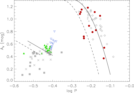
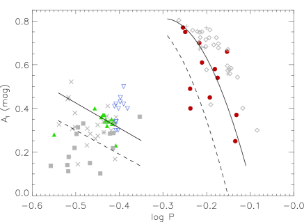
Figure 17: Bailey diagram of the light curve amplitude $A$ against $\log P$ for RRL stars in M68, in the $V$ (top) and $I$ (bottom) bands. The locations of confirmed RRL stars are marked in red with filled circles (RR0), green filled triangles (RR1) and blue open inverted triangles (RR01). For the RR01 stars, the amplitude is that of the dominant mode, which is the first overtone in all cases here. For the $V-$band diagram, we also plot the tracks derived by Zorotovic et al. (2010) for evolved stars (solid lines), found by shifting the relations obtained by fitting data for the Oosterhoff type I cluster M3 (dashed lines) by 0.06 in $\log P$. For the $I-$band diagram, we plot the rescaling of those relations by Kunder et al. (2013b) for Oosterhoff type I (dashed lines) and type II (solid lines) clusters. On both diagrams we also plot the RRL stars in Oosterhoff type II clusters NGC 5024 (Arellano Ferro et al. 2011) and M9 (Arellano Ferro et al. 2013a) in light grey. For those, RR0 and RR1 stars are plotted as open diamonds and filled squares respectively, with RRL stars exhibiting Blazhko modulation plotted as + signs (RR0) and crosses (RR1). One double-mode star is also plotted as an asterisk.

6.2 Cluster metallicity

Although Clement et al. (2001), found a correlation between the metallicity of a globular cluster and the mean period of its RR0 stars, $\langle P_{\rm RR0}\rangle$, they noted that this relation does not hold when $\langle P_{\rm RR0}\rangle$ is larger than 0.6 d, i.e. for Oosterhoff type II clusters. Instead, we estimate the metallicity of M68 by calculating the average of the metallicities we derived for RRL stars in this cluster. As in our previous papers (e.g. Kains et al. 2013), we assume that there is no systematic offset between the metallicities derived for RR0 and RR1 stars. Using this method, we find a mean metallicity of $\mathrm{[Fe/H]_{ZW}}=-2.07\pm 0.06$ (using Eq. (9) to derive RR0 metallicities) and $\mathrm{[Fe/H]_{ZW}}=-2.13\pm 0.11$ (using Eq. (10)), corresponding to $\mathrm{[Fe/H]_{UVES}}=-2.20\pm 0.10$ and $\mathrm{[Fe/H]_{UVES}}=-2.30\pm 0.17$ respectively. Both values are in excellent agreement with the value of Carretta et al. (2009b), who found $\mathrm{[Fe/H]_{UVES}}=-2.27\pm 0.01\pm 0.07$ (statistical and systematic errors respectively), and with most values in the literature, listed in Table 9. In the rest of this paper, we will use $\mathrm{[Fe/H]_{ZW}}=-2.07\pm 0.06$ as the cluster metallicity, due to the larger scatter in RR0 metallicities derived using Eq. (10), and the problem with uncertainties in the relation of Nemec et al. (2013) already mentioned in Sec. 4.1.

Reference	$\mathrm{[Fe/H]_{ZW}}$	$\mathrm{[Fe/H]_{UVES}}$	Method
This work	$-2.07\pm 0.06$	$-2.20\pm 0.10$	Fourier decomposition of RRL light curves
This work	$-2.09\pm 0.26$	$-2.24\pm 0.42$	$M_{V}-$[Fe/H] relation
Carretta et al. (2009b)	-2.10 $\pm$ 0.04	$-2.27\pm 0.07$	UVES spectroscopy of red giants
Carretta et al. (2009c)	-2.08 $\pm$ 0.04	$-2.23\pm 0.07$	FLAMES/GIRAFFE spectra of red giants
Rutledge et al. (1997)	-2.11 $\pm$ 0.03	$-2.27\pm 0.05$	CaII triplet
Harris (1996)	-2.23	-2.47	Globular cluster catalogue
Suntzeff et al. (1991)	-2.09	-2.24	Spectroscopy of RR Lyrae/ $\Delta$S index
Gratton & Ortolani (1989)	-1.92 $\pm$ 0.06	$-1.97\pm 0.09$	High-resolution spectroscopy
Minniti et al. (1993)	-2.17 $\pm$ 0.05	$-2.37\pm 0.08$	FeI and FeII spectral lines
Zinn & West (1984)	-2.09 $\pm$ 0.11	$-2.24\pm 0.18$	$Q_{39}$ index
Zinn (1980)	-2.19 $\pm$ 0.06	$-2.41\pm 0.10$	$Q_{39}$ index

Table 9: Different metallicity estimates for M68 in the literature. Values were converted using Eq. (11) where necessary.

6.3 Reddening

Individual RR0 light curves can be used to estimate the reddening to each star, using their colour near the point of minimum brightness. The method was first proposed by Sturch (1966), and further developed in several studies, most recently by Guldenschuh et al. (2005) and Kunder et al. (2010). Guldenschuh et al. (2005) find that the intrinsic $(V-I)_{0}$ colour of RR0 stars between phases 0.5 and 0.8 is $(V-I)_{0}^{\phi[0.5-0.8]}=0.58\pm 0.02$ mag. By calculating the $(V-I)$ colour for each of our light curves between those phases and comparing it to the value of Guldenschuh et al. (2005), we can therefore calculate values of $E(V-I)$, which we can then convert through $E(B-V)=E(V-I)/1.616$ (e.g. Arellano Ferro et al. 2013a). Stars showing Blazhko modulation were excluded from this calculation, as were stars with poor $I-$band light curves, leading to reddening estimates for V2, V12, V14, V22, V23, V35 and V46. We found a mean reddening of $0.05\pm 0.05$ mag, within the range of values published (see Sec. 6.4.1).

6.4 Distance

6.4.1 Using the RRL stars

The Fourier decomposition of RRL stars can also be used to derive a distance modulus to the cluster. The Fourier fit parameter $A_{0}$ corresponds to the intensity-weighted mean $V$ magnitude of the light curve, and since we also derived absolute magnitudes for each star with a good Fourier decomposition, this can be used to calculate the distance modulus to each star.

For RR0 stars, the mean value of $A_{0}$ is $15.64\pm 0.08$ mag, while the mean absolute value is $\langle M_{V}\rangle=0.49\pm 0.07$ mag. From this, we find a distance modulus $\mu=15.15\pm 0.11$ mag. For RR1 stars, we find $\langle A_{0}\rangle=15.68\pm 0.03$ mag and $\langle M_{V}\rangle=0.53\pm 0.01$ mag, yielding $\mu=15.15\pm 0.03$ mag.

Many values of $E(B-V)$ have been published for M68, ranging from 0.01 mag (e.g. Racine 1973) to 0.07 mag (e.g. Bica & Pastoriza 1983). Recent studies have tended to use $E(B-V)=0.05$ mag, which is the value listed in the catalogue of Harris (1996). Piersimoni et al. (2002) derived a value of $E(B-V)=0.05\pm 0.01$ from $BVI$ photometry of RRL stars and empirical relations, and this coincides with the value we derived in Sec. 6.3, although uncertainties on our estimate are larger. We therefore adopt the value of Piersimoni et al. (2002), and a value of $R_{V}=3.1$ for the Milky Way. From this we find true distance moduli of $\mu_{0}=15.00\pm 0.11$ mag and $\mu_{0}=15.00\pm 0.05$ mag from RR0 and RR1 stars, respectively. These values correspond to physical distances of $10.00\pm 0.49$ kpc and $9.99\pm 0.21$ kpc, respectively, and are consistent with values reported in the literature, examples of which we list in Table 10.

6.4.2 Using SX Phoenicis stars

We can derive distances to SX Phe stars thanks to empirical period-luminosity ($P-L$) relations (e.g. Jeon et al. 2003). Here we calculate distances to the SX Phe stars in our images (see Table 3) using the $P-L$ relation of Cohen & Sarajedini (2012),

$$M_{V}=-(1.640\pm 0.110)-(3.389\pm 0.090)\log P_{f}\,,$$ (24)

where $P_{f}$ is the fundamental-mode pulsation period. This provides us with another independent estimate of the distance to M68. Arellano Ferro et al. (2011) derived their own $P-L$ relation, using only SX Phe stars in metal-poor globular clusters, and have shown a good match of their relation to the locus of SX Phe in other clusters (e.g. Arellano Ferro et al. 2014, 2013b).

Assuming that the values given in Table 3 are the fundamental periods and using them with Eq. (24) as well as the relation of Arellano Ferro et al. (2011), the distances derived for V39, V48, V51 and V52 disagree with the values we found using RRL stars, and with most values in the literature (see Table 10). In Fig. 18, we plot $\log P$ against dereddened magnitudes $V_{0}$ (using our adopted value $E(B-V)=0.05\pm 0.01$ mag), as well as the relations of Cohen & Sarajedini (2012) for fundamental, first and second overtone SX Phe pulsators, shifted to a distance of $9.99\pm 0.21$ kpc, the cluster distance we derived in Sec. 6.4.1 using RR1 stars. From this, it is clear that V49 pulsates in the fundamental mode, and that the periods of the double-mode pulsator V50 (see Sec. 5.2) do correspond to fundamental and first-overtone periods. Fig. 18 also suggests that V51 and V52 are first-overtone pulsators, and that V48 is a second-overtone pulsator; W94 had suggested that V48 might be a first-overtone pulsator, noting however that it would be bright for its period. Fig. 18 also suggest that V39 might not be a cluster member, with the large distance hinting that it may be a background object.

For the overtone pulsators, we can “fundamentalise” the periods to then use Eq. (24) in order to derive empirical values of $M_{V}$, $\mu_{0}$, and the distance. To do this, we use the canonical first- and second-overtone to fundamental period ratios, respectively $P_{1}/P_{f}\sim 0.783$ (e.g. Jeon et al. 2004; Santolamazza et al. 2001; Gilliland et al. 1998) and $P_{2}/P_{f}\sim 0.62$ (Santolamazza et al. 2001). Using these values to calculate $P_{f}$, we find the corrected absolute magnitudes and distances listed in Table 11.

We note that the discrepant distance estimates could alternatively be due to V48 being a foreground object, while V51 clearly suffers from blending from two nearby stars of comparable brightness, meaning that its reference flux could be over-estimated by as much as a factor of 2. If this is the case, V51 would fall on the track for fundamental pulsators on Fig. 18. Higher-resolution data could help determine which explanation is correct for V51, while radial velocity measurements would help address the cluster membership of V39 and V48.

Using the corrected values, and excluding V39, we find an average distance modulus of $\mu_{0}=14.97\pm 0.11$ mag, corresponding to a physical distance of $9.84\pm 0.50$ kpc, in good agreement with the values we found using RRL stars in the previous section.

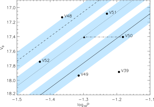
Figure 18: $\log P-V_{0}$ plot of the SX Phe stars in M68, with the $P-L$ relation of Cohen & Sarajedini (2012) for fundamental, first-overtone, and second-overtone pulsators as solid, dotted, and dashed lines respectively. Shaded areas show 1-$\sigma$ boundaries for each case. The relations have been shifted to a distance of $9.99\pm 0.21$ kpc (see Sec. 6.4.1), and the SX Phe magnitudes have been dereddened using our adopted value of $E(B-V)=0.05\pm 0.01$ mag. The location of the black filled circles in this plot correspond to the periods listed in Table 3, and for V50 the first-overtone period is shown as a triangle, with a dash-dot line connecting the two periods.

Reference	$\mu_{0}$ [mag]	Distance [kpc]	Method
This work	$15.00\pm 0.11$	$10.00\pm 0.49$	Fourier decomposition of RR0 light curves
This work	$15.00\pm 0.05$	$9.99\pm 0.21$	Fourier decomposition of RR1 light curves
This work	$14.97\pm 0.11$	$9.84\pm 0.50$	SX Phe $P-L$ relation
This work	$15.00\pm 0.07$	$10.00\pm 0.30$	$M_{V}-$[Fe/H] relation for cluster RRL stars
Rosenberg et al. (1999)	15.02	10.07	CMD analysis
Caloi et al. (1997)	15.15	10.72	CMD isochrone fitting
Brocato et al. (1997)	15.16 $\pm$ 0.10	$10.76\pm 0.50$	CMD isochrone fitting
Gratton et al. (1997)	15.24 $\pm$ 0.08	$11.17\pm 0.41$	CMD analysis
Harris (1996)	15.06	10.3	Globular cluster catalogue
Straniero & Chieffi (1991)	14.99 $\pm$ 0.03	9.94 $\pm$ 0.14	CMD isochrone fitting
McClure et al. (1987)	15.03 $\pm$ 0.15	10.14 $\pm$ 0.70	CMD analysis
Alcaino (1977)	14.97	9.8	Magnitude of the HB
Harris (1975)	14.91	9.6	Mean magnitude of RRL stars

Table 10: Distance modulus and physical distance estimates for M68 in the literature.

Reference	$M_{V}[mag]$	$\mu_{0}$ [mag]	Distance [kpc]
V39	2.40$\pm$0.11	15.48$\pm$0.25	12.48$\pm$1.42
V48	2.28$\pm$0.11	14.86$\pm$0.13	9.35$\pm$0.55
V49	2.81$\pm$0.11	15.12$\pm$0.21	10.57$\pm$1.03
V50	2.36$\pm$0.11	14.04$\pm$0.15	10.19$\pm$0.73
V51	2.17$\pm$0.11	14.92$\pm$0.14	9.63$\pm$0.64
V52	2.85$\pm$0.11	14.89$\pm$0.14	9.53$\pm$0.60

Table 11: Absolute magnitudes, true distance moduli and physical distance for the SX Phe stars in M68, derived using the $P-L$ relation of Cohen & Sarajedini (2012) after “fundamentalisation” of the pulsation period.

6.5 Distance and metallicity from the $M_{V}-$[Fe/H] relation

Many studies in the literature have compiled magnitude and metallicity measurements from globular cluster observations to fit a linear relation between the metallicity of a cluster and the mean magnitude of its RRL stars, $M_{V}=\alpha{\rm[Fe/H]}\,+\beta$. Here we use the relation derived by Kains et al. (2012), with coefficients $\alpha=0.16\pm 0.01$ and $\beta=0.85\pm 0.02$, for a metallicity given on the ZW scale. Using the metallicity value of $\mathrm{[Fe/H]_{ZW}}=-2.07\pm 0.06$ derived in Sec. 6.2, we find a mean absolute magnitude of $0.52\pm 0.03$ mag, in good agreement with the value found in Sec. 6.4.1. We can now use this to estimate the distance to M68, in a similar way to what was done in that section. Since the $M_{V}-$[Fe/H] does not distinguish between RR0 and RR1, we use average value over all RRL types in this calculation.

We find a mean magnitude for all RRL stars of $\langle A_{0}\rangle=15.68\pm 0.05$ mag, yielding a distance modulus of $\mu=15.16\pm 0.06$ mag. With $E(B-V)=0.05\pm 0.01$ mag and $R_{V}=3.1$ as in Sec. 6.4.1, this gives a true distance modulus of $15.00\pm 0.07$ mag, corresponding to a physical distance of $10.00\pm 0.30$ kpc.

Conversely, we can also estimate the mean metallicity of the cluster using the $M_{V}-$[Fe/H] relation, using the values found from Eqs. (17) and (18). We find a mean value for all RRL stars with a good Fourier decomposition of $M_{V}=0.52\pm 0.04$, yielding $\mathrm{[Fe/H]_{ZW}}=-2.09\pm 0.26$, in agreement with our values in Sec. 6.2, but with a much larger error bar.

6.6 Age

Although our CMD does not allow us to derive a precise age, we use our data to check consistency of our CMD with age estimates of M68 from the literature (Table 12), by overplotting the isochrones of Dotter et al. (2008), using our estimate of the cluster metallicity of $\mathrm{[Fe/H]_{ZW}}=-2.07\pm 0.06$. We interpolated those isochrones to match the alpha-element abundance for this cluster of [$\alpha$/Fe] of $\sim 0.3$ (e.g. Carney 1996). We found that our CMD is consistent with an age of $13.0\pm 0.50$ Gyr, in agreement with the most recent values in the literature.

Reference	Age [Gyr]	Method
VandenBerg et al. (2013)	12.00$\pm$0.25	CMD isochrone fitting
Rakos & Schombert (2005)	11.2	Strömgren photometry
Salaris & Weiss (2002)	11.2 $\pm$ 0.9	CMD analysis
Caloi et al. (1997)	12 $\pm$ 2	CMD analysis
Gratton et al. (1997)	10.1 $\pm$ 1.2	CMD isochrone fitting
Gratton et al. (1997)	11.4 $\pm$ 1.4	CMD isochrone fitting
Brocato et al. (1997)	10	CMD analysis
Jimenez et al. (1996)	12.6 $\pm$ 2	CMD analysis
Chaboyer et al. (1996)	12.8 $\pm$ 0.3	CMD analysis
Sandage (1993)	12.1 $\pm$ 1.2	CMD isochrone fitting
Straniero & Chieffi (1991)	19 $\pm$ 1	CMD isochrone fitting
Alcaino et al. (1990)	13 $\pm$ 3	CMD isochrone fitting
Chieffi & Straniero (1989)	16	CMD isochrone fitting
McClure et al. (1987)	14 $\pm$ 1	CMD isochrone fitting
Peterson (1987)	15.5	CMD analysis
Vandenberg (1986)	18	CMD analysis

Table 12: Age estimates for M68 in the literature.

7 Conclusions

We carried out a detailed survey of variability in M68 using CCD observations as well as some EMCCD images. We showed that data from identical telescopes in a telescope network could be reduced using a reference image from a single telescope, i.e. that the network could be considered to be a single telescope for the purposes of data handling. This facilitates the analysis of time-series data taken with such networks significantly.

Using our observations we were able to recover all known variables within our field of view, as well as to detect four new SX Phe variables near the cluster core. We used the light curves of RRL stars in our data to derive estimates for their metallicity, effective temperature, luminosity and mean mass. Those were then used to infer values for the cluster metallicity, reddening and distance. Furthermore, the light curves of the SX Phe stars were also used to obtain an additional independent estimate of distance.

We found a metallicity [Fe/H]=$-2.07\pm 0.06$ on the ZW scale and $-2.20\pm 0.10$ on the UVES scale. We derived distance moduli of $\mu_{0}=15.00\pm 0.11$ mag (using RR0 stars), $\mu_{0}=15.00\pm 0.05$ mag (using RR1 stars), $\mu_{0}=14.97\pm 0.11$ mag (using SX Phe stars), and $\mu_{0}=15.00\pm 0.07$ mag (using the $M_{V}-$[Fe/H] relation for RRL stars), corresponding to physical distances of $10.00\pm 0.49$, $9.99\pm 0.21$, $9.84\pm 0.50$, and $10.00\pm 0.30$ kpc, using RR0, RR1, SX Phe stars, and the $M_{V}-$[Fe/H] relation respectively. Finally, we used our CMD to check the consistency of age estimates in the literature for M68. We also used archival data to refine period estimates, and calculate period changes where appropriate, for the RRL stars. The grid search we used here is particularly useful to estimate period changes for stars for which not many maxima were observed; in those cases, the traditional O-C method struggles to yield a period-change value that phases all data sets well, while the grid search performs better. We also examined in detail the light curves of double-mode pulsators in this cluster. The ratios of the RR01 periods enabled us to estimate their masses with the new mass-period-metallicity empirical relation of Marconi et al. (2015, submitted).

Thanks to the latest DIA methods, we can now be confident that all of the RRL stars in M68 are known. Carrying out such studies for more Milky Way globular clusters will help us strengthen observational evidence for the Oosterhoff dichotomy, which in turn can be used to shed light on the origin of the Galactic halo.

References

- Alard (1999) Alard, C. 1999, A&A, 343, 10
- Alard (2000) Alard, C. 2000, Astron. Astrophys. Suppl. Ser., 144, 363
- Albrow et al. (2009) Albrow, M. D., Horne, K., Bramich, D. M., et al. 2009, MNRAS, 397, 2099
- Alcaino (1977) Alcaino, G. 1977, Astron. Astrophys. Suppl. Ser., 29, 9
- Alcaino et al. (1990) Alcaino, G., Liller, W., Alvarado, F., & Wenderoth, E. 1990, AJ, 99, 1831
- Arellano Ferro et al. (2014) Arellano Ferro, A., Ahumada, J. A., Calderón, J. H., & Kains, N. 2014, Rev. Max. Astron. Astrofis., 50, 307
- Arellano Ferro et al. (2013a) Arellano Ferro, A., Bramich, D. M., Figuera Jaimes, R., et al. 2013a, MNRAS, 434, 1220
- Arellano Ferro et al. (2013b) Arellano Ferro, A., Bramich, D. M., Giridhar, S., et al. 2013b, Act. Astron., 63, 429
- Arellano Ferro et al. (2011) Arellano Ferro, A., Figuera Jaimes, R., Giridhar, S., et al. 2011, MNRAS, 416, 2265
- Arellano Ferro et al. (2010) Arellano Ferro, A., Giridhar, S., & Bramich, D. M. 2010, MNRAS, 402, 226
- Arellano Ferro et al. (2008) Arellano Ferro, A., Rojas López, V., Giridhar, S., & Bramich, D. M. 2008, MNRAS, 384, 1444
- Bellini et al. (2011) Bellini, A., Anderson, J., & Bedin, L. R. 2011, PASP, 123, 622
- Belserene (1964) Belserene, E. P. 1964, AJ, 69, 475
- Benedict et al. (2002) Benedict, G. F., McArthur, B. E., Fredrick, L. W., et al. 2002, AJ, 123, 473
- Bessell (2005) Bessell, M. S. 2005, ARA&A, 43, 293
- Bica & Pastoriza (1983) Bica, E. L. D. & Pastoriza, M. G. 1983, Astrophysics & Space Science, 91, 99
- Blažko (1907) Blažko, S. 1907, Astronomische Nachrichten, 175, 325
- Bono et al. (2003) Bono, G., Caputo, F., Castellani, V., et al. 2003, MNRAS, 344, 1097
- Bragaglia et al. (2001) Bragaglia, A., Gratton, R. G., Carretta, E., et al. 2001, AJ, 122, 207
- Bramich (2008) Bramich, D. M. 2008, MNRAS, 386, L77
- Bramich et al. (2011) Bramich, D. M., Figuera Jaimes, R., Giridhar, S., & Arellano Ferro, A. 2011, MNRAS, 413, 1275
- Bramich & Freudling (2012) Bramich, D. M. & Freudling, W. 2012, MNRAS, 424, 1584
- Bramich et al. (2013) Bramich, D. M., Horne, K., Albrow, M. D., et al. 2013, MNRAS, 428, 2275
- Brocato et al. (1997) Brocato, E., Castellani, V., & Piersimoni, A. 1997, ApJ, 491, 789
- Brocato et al. (1994) Brocato, E., Castellani, V., & Ripepi, V. 1994, AJ, 107, 622
- Cacciari et al. (2005) Cacciari, C., Corwin, T. M., & Carney, B. W. 2005, AJ, 129, 267
- Caloi et al. (1997) Caloi, V., D’Antona, F., & Mazzitelli, I. 1997, A&A, 320, 823
- Carney (1996) Carney, B. W. 1996, PASP, 108, 900
- Carretta et al. (2009a) Carretta, E., Bragaglia, A., Gratton, R., D’Orazi, V., & Lucatello, S. 2009a, A&A, 508, 695
- Carretta et al. (2009b) Carretta, E., Bragaglia, A., Gratton, R., & Lucatello, S. 2009b, A&A, 505, 139
- Carretta et al. (2009c) Carretta, E., Bragaglia, A., Gratton, R. G., et al. 2009c, A&A, 505, 117
- Castelli (1999) Castelli, F. 1999, A&A, 346, 564
- Catelan (2009) Catelan, M. 2009, Astrophysics & Space Science, 320, 261
- Chaboyer et al. (1996) Chaboyer, B., Demarque, P., Kernan, P. J., Krauss, L. M., & Sarajedini, A. 1996, MNRAS, 283, 683