Long term variability of Cygnus X-1:

Binary systems with an accreting compact object are a unique chance to investigate the strong, clumpy, line-driven winds of early type supergiants by using the compact object’s X-rays to probe the wind structure. We analyze the two-component wind of HDE 226868, the O9.7Iab giant companion of the black hole Cyg X-1 using 4.77 Ms of RXTE observations of the system taken over the course of 16 years. Absorption changes strongly over the 5.6 d binary orbit, but also shows a large scatter at a given orbital phase, especially at superior conjunction. The orbital variability is most prominent when the black hole is in the hard X-ray state. Our data are poorer for the intermediate and soft state, but show signs for orbital variability of the absorption column in the intermediate state. We quantitatively compare the data in the hard state to a toy model of a focussed Castor-Abbott-Klein-wind: as it does not incorporate clumping, the model does not describe the observations well. A qualitative comparison to a simplified simulation of clumpy winds with spherical clumps shows good agreement in the distribution of the equivalent hydrogen column density for models with a porosity length on the order of the stellar radius at inferior conjunction; we conjecture that the deviations between data and model at superior conjunction could be either due to lack of a focussed wind component in the model or a more complicated clump structure.

1 Introduction

Early type supergiants show strong line driven winds (CAK mechanism; Castor, Abbott, & Klein 1975; Morton 1967; Lucy & Solomon 1970) and typical mass loss rates of a few $10^{-6}M_{\odot}/\mathrm{yr}$ (e.g., Puls et al. 2006). These high velocity winds that can reach terminal velocities $\varv_{\infty}>2000\,\mathrm{km}\,\mathrm{s}^{-1}$ (e.g., Muijres et al. 2012) are perturbed and clumpy (Owocki et al. 1988; Feldmeier et al. 1997; Puls et al. 2006; Oskinova et al. 2012; Sundqvist & Owocki 2013) with over 90% of the wind mass concentrated in less than $\sim$10% of the wind volume (Sako et al. 1999; Rahoui et al. 2011, for Vela X-1 and Cyg X-1, respectively). Binary systems consisting of an O/B type giant and a compact object offer us the unique chance to investigate these winds by using the X-ray source as a test probe.

Cygnus X-1 is in such a high mass X-ray binary with the O9.7Iab supergiant HDE 226868 (Walborn 1973). Located $\sim$1.86 kpc away (Reid et al. 2011, see also Xiang et al. 2011), it is one of the brightest and best-observed black hole binaries. The orbital period is $P=5.599829\pm 0.000016$ d with $T_{0}=52872.288\pm 0.009$ (Gies et al. 2008). The source also shows a superorbital period that has been reported as $\sim$300 d (Priedhorsky et al. 1983), then as $\sim$150 d (Brocksopp et al. 1999; Benlloch et al. 2004; Ibragimov et al. 2007), and lately as having changed back to $\sim$300 d (Zdziarski et al. 2011).

The intrinsic variability of Cyg X-1 on timescales of hours (Böck et al. 2011) to years (Pottschmidt et al. 2003; Wilms et al. 2006; Shaposhnikov & Titarchuk 2006; Axelsson et al. 2006; Grinberg et al. 2013) can be classified in terms of X-ray spectral states that also show distinct timing characteristics on timescales below 1 s and are similar for most black hole binaries (for a review see, e.g., Belloni 2010). In particular, the hard state spectrum above $\sim$2 keV is dominated by a power law component with photon index $\Gamma\sim 1.7$, while in the soft state the thermal emission from the accretion disk is prominent and the contribution from a steeper power law component is low.

Orosz et al. (2011) determine the inclination of the binary system to $i=27\aas@@fstack{\circ}{}1\pm 0\aas@@fstack{\circ}{}8$, the black hole mass to $M_{\mathrm{BH}}=(14.8\pm 1.0)M_{\odot}$, and the companion mass to $M_{\mathrm{\star}}=(19.2\pm 1.9)M_{\odot}$, the latter value being questioned by Ziółkowski (2014), who estimate a range of 25–35 $M_{\odot}$ with a most likely value of 27 $M_{\odot}$. As HDE 226868 fills $\gtrsim$90% of its Roche lobe (Gies et al. 2003) and has a strong (a few $10^{-6}$ $M_{\odot}\,\mathrm{yr}^{-1}$, Gies et al. 2003) fast wind, the black hole accretes via a focussed wind (Friend & Castor 1982; Gies & Bolton 1986a, b; Sowers et al. 1998; Miller et al. 2005; Hanke et al. 2009; Hell et al. 2013; Miškovičová et al. 2015, and others). Values for $\varv_{\infty}$ for HDE 226868 vary in the literature: Davis & Hartmann (1983) obtain $(2300\pm 400)\,\mathrm{km}\,\mathrm{s}^{-1}$ in the hard state, but Vrtilek et al. (2008) $1420\,\mathrm{km}\,\mathrm{s}^{-1}$ in the soft state. Herrero et al. (1995) adopt $2100\,\mathrm{km}\,\mathrm{s}^{-1}$. Gies et al. (2008) obtain $1200\,\mathrm{km}\,\mathrm{s}^{-1}$ during a soft state, but list $1600\,\mathrm{km}\,\mathrm{s}^{-1}$ as more likely.

The inclination of the system implies that our line of sight probes different regions of the wind at different orbital phases. Orbital variability of the absorption column density in the hard state has been reported by Feng & Cui (2002), Ibragimov et al. (2005), and Boroson & Vrtilek (2010). Dips in the (soft) X-ray lightcurves of Cyg X-1 are interpreted as signatures of clumps in the stellar wind. They occur preferably at superior conjunction ($\phi_{\mathrm{orb}}\sim 0$), i.e., when the O-star companion is between the observer and the black hole (e.g., Li & Clark 1974; Mason et al. 1974; Parsignault et al. 1976; Pravdo et al. 1980; Remillard & Canizares 1984; Kitamoto et al. 1984; Bałucińska-Church et al. 2000; Poutanen et al. 2008; Boroson & Vrtilek 2010).

The 16 years of mainly bi-weekly Cyg X-1 observations (1996–2011) with RXTE’s Proportional Counter Array (PCA; Jahoda et al. 2006) and High Energy X-ray Timing Experiment (HEXTE; Rothschild et al. 1998) allowed us to study the long-term spectral and X-ray timing evolution of the source in unprecedented detail in the previous paper of the series (Pottschmidt et al. 2003; Gleissner et al. 2004b, a; Wilms et al. 2006; Grinberg et al. 2013, 2014). In this paper, we use these data to analyze the orbital variability of absorption due to the focussed wind. The exceptional exposure reveals subtle effects such as the orbital variability in intermediate states and rare events with very high absorption.

In Sect. 2, we introduce the data used and the spectral models applied to describe them. In Sect. 3, we discuss the observed orbital variability of absorption in hard, intermediate, and soft states. In Sect. 4, we compare our measurements with previous results and with different wind models, namely with a toy model for a CAK-wind and with simulations of clumpy winds in single stars. We summarize our results in Sect. 5.

2 Data and spectral analysis

Ibragimov et al. (2005) used 42 Ginga-OSSE and RXTE-OSSE observations of Cyg X-1 taken mainly in the hard state to show orbital variability of absorption by demonstrating an increased equivalent hydrogen column density, $N_{\mathrm{H}}$, around $\phi_{\mathrm{orb}}\sim 0$. In Wilms et al. (2006), we analyzed 202 observations from 1999–2004 using RXTE-PCA and, where available, -HEXTE spectra with models similar to the one presented below and with a time resolution of individual RXTE observations that were typically of several satellite orbits in length, i.e., had exposure times of 5–10 ks. Boroson & Vrtilek (2010) classified 102 of these observations as hard states and used them to demonstrate the orbital variability of absorption in the hard state, but did not have enough data taken during softer states. At the same time, higher sensitivity snapshots at different $\phi_{\mathrm{orb}}$ with Chandra (Miller et al. 2005; Hanke et al. 2009; Hanke 2011; Miškovičová et al. 2015) and Suzaku (Nowak et al. 2011; Miller et al. 2012; Yamada et al. 2013) revealed a complex structure of the wind with highly variable local densities, but the orbital coverage was significantly worse than the RXTE measurements.

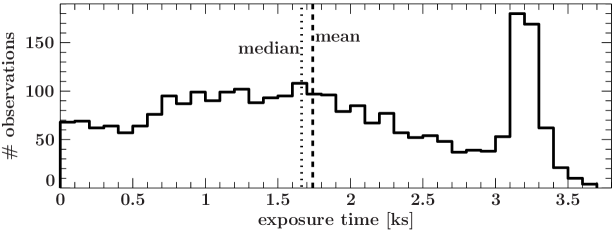
Figure 1: Histogram of the PCA exposure times of the individual satellite orbit-wise observations analyzed in this work. The mean exposure is 1.74 ks, the median 1.66 ks.

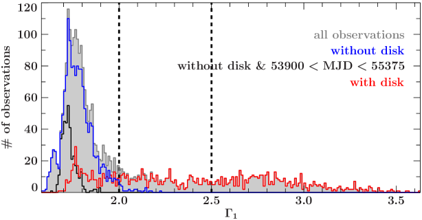
Figure 2: Number of orbitwise PCA observations with a given soft photon index $\Gamma_{1}$ that do (red) or do not (blue) require a multitemperature disk component. Additionally highlighted are observations that do not require a disk and fall into the long hard state of MJD 53900–55375 (black). Dashed vertical lines indicate thresholds for hard ($\Gamma_{1}\leq 2.0$), intermediate ($2.0<\Gamma_{1}\leq 2.5$) and soft ($2.5<\Gamma_{1}$) states according to Grinberg et al. (2013).

In this paper we therefore extend the earlier RXTE analyses, using the full mission-long database of RXTE observations of Cyg X-1, and using spectra taken with the exposure of one orbit of the RXTE satellite around Earth, or around 1.6 ks (Fig. 1). We thus probe average spectral parameters on shorter timescales than earlier RXTE studies over a variety of spectral shapes (Fig. 2). Our total sample consists of 2741 PCU 2 and HEXTE-spectra (Grinberg et al. 2013). The total exposure time of our observations is 4.77 Ms which corresponds to almost 10 fully covered orbital periods of 5.6 d. The exposure is evenly distributed between the orbital phases. Advances in PCA calibration (Shaposhnikov et al. 2012) and a careful consideration of energy-dependent systematic uncertainties in different gain epochs of the PCA-instrument (Hanke 2011; Grinberg et al. 2013) strengthen our analysis. For a detailed discussion of data treatment, see Grinberg et al. (2013). All analyses in this paper were performed with ISIS 1.6.2 (Houck & Denicola 2000; Houck 2002; Noble & Nowak 2008).

In performing our analysis we used the same approach as that employed by us previously (Grinberg et al. 2013), i.e., we model the data empirically with a broken power law with soft photon index $\Gamma_{1}$, hard photon index $\Gamma_{2}$, and a spectral break at $\sim$10 keV (Wilms et al. 2006). This broken power law is modified by a high-energy cutoff, by an Fe K$\alpha$-line modelled with a Gaussian at $\sim$6.4 keV, and by absorption. A multitemperature disk (diskbb, Mitsuda et al. 1984; Makishima et al. 1986) is added to the model where it improves the $\chi^{2}$ by more than 5% except in seven cases where the X-ray timing behavior and the correlation between $\Gamma_{1}$ and $\Gamma_{2}$ strongly prefer the model without a disk (Grinberg et al. 2014). Figure 3 shows that the model offers a very good description of the spectrum. As in Grinberg et al. (2013), we use $\Gamma_{1}$-based state definitions derived from spectral and timing properties of Cyg X-1: the source is in hard state if $\Gamma_{1}\leq 2.0$, in the intermediate state if $2.0<\Gamma_{1}\leq 2.5$ and in the soft state if $2.5<\Gamma_{1}$. The distribution of observations with $\Gamma_{1}$ is shown in Fig. 2. Out of 1822 hard state observations, 1515 do not require a disk, but 384 out of 413 intermediate state observations and all 506 soft state observations require a disk component.

When studying variations of $N_{\mathrm{H}}$ in an astronomical source, the measured column towards the source consists of two main components: absorption in the interstellar medium (ISM) that is constant on observable timescales and a variable absorption local to the X-ray source. For Galactic sources, X-ray data do not allow us to distinguish the two absorption components. In the case of Cyg X-1, we therefore take the constant ISM contribution into account by setting a minimum value for $N_{\mathrm{H}}$ to $N_{\mathrm{H,ISM}}=4.8\times 10^{21}\,\mathrm{cm}^{-2}$, as derived by Xiang et al. (2011) from studies of the dust scattering halo of the source. We describe absorption with the tbnew model, an improved version of tbabs (Wilms et al. 2000), using wilm abundances of Wilms et al. (2000) and vern cross sections of Verner et al. (1996). Note that optical depth at a frequency $\nu$ depends on the total cross-section $\sigma_{\nu}$ and the hydrogen column density $N_{\mathrm{H}}$ as $\tau_{\nu}=\sigma_{\nu}\cdot N_{\mathrm{H}}$. The observed spectrum, $I_{\mathrm{obs}}$, and the source spectrum, $I_{\mathrm{src}}$, are then related by $I_{\mathrm{obs},\nu}=I_{\mathrm{src},\nu}\cdot e^{-\tau_{\nu}}$. For the individual contribution to $\sigma_{\nu}$ from different phases of the absorbing medium (e.g., gas or dust) and the different constituents (e.g., oxygen) see Wilms et al. (2000) or Gatuzz et al. (2015). Generally in the X-ray range, the optical depth is dominated by metals (Wilms et al. 2000) and $\sigma_{\nu}\propto E^{-3}$, i.e., the photoelectric absorption acts more strongly on the low energy photons.

We caution that the exact choice of absorption model, abundances, and cross-sections can lead to differences in $N_{\mathrm{H}}$ up to 20%–30% between different approaches (Wilms et al. 2000), although they do not affect overall trends observed. We also caution that the absorption modeling is based on the absorption of neutral material, while in reality the material will be moderately photoionized by the strong X-ray source embedded in it. Especially when using proportional counters such as the PCUs, approximating the X-ray absorption by ionized material with absorption in neutral material is an appropriate assumption, since most absorption is due to K-shell absorption, which is only mildly dependent on ionization stage. However, our modelling will not pick up effects from fully ionized material, as it is mainly transparent to X-rays and RXTE’s instruments did not have the resolution to detect absorption lines.

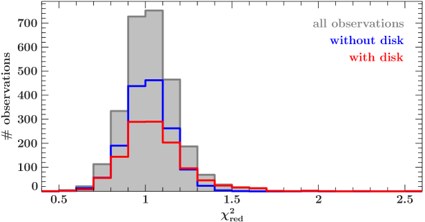
Figure 3: Histogram of $\chi^{2}_{\mathrm{red}}$ values for observations that do (red) and do not (blue) require a multitemperature disk component.

A second issue relates to the uncertainty of the $N_{\mathrm{H}}$ measurements. For models such as the ones used here there is a well known degeneracy between the power law slope, i.e., $\Gamma_{1}$, and $N_{\mathrm{H}}$ (e.g., Suchy et al. 2008). By calculating two-dimensional confidence contours we confirm that this degeneracy is not responsible for the variation of $N_{\mathrm{H}}$ discussed here (for example contours see Hanke 2011). Because of the limited energy range of the PCA, in addition to the correlation with the power law continuum there is also a degeneracy between parameters of the accretion disk and $N_{\mathrm{H}}$. The effect of a stronger absorption can be counterweighted by a stronger disk component and vice versa. $N_{\mathrm{H}}$-values from best fit models with and without a disk therefore have to be considered separately because of the different systematic effects and we do so throughout this paper. Unless discussed otherwise, we give all uncertainties at the 90% level.

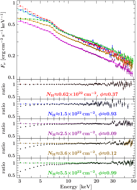
Figure 4: Example spectra with $1.72<\Gamma_{1}<1.73$, but different absorption columns. PCA data and best fit models to PCA and HEXTE data are shown. The ratio plots show residuals of the best fit in color and residuals of an evaluation of the best fit model with $N_{\mathrm{H}}=N_{\mathrm{H,ISM}}$ (i.e., no absorption local to the system) in black. All observations are from the hard state of 2006–2010 (Sect. 3.1).

3 Orbital variability of absorption

3.1 Hard state

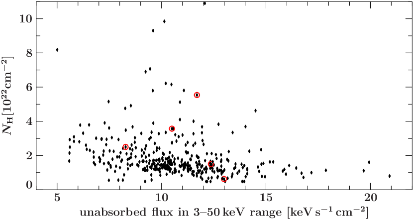
Figure 5: Absorption column vs. unabsorbed energy flux during the hard state of 2006–2010. Red circles mark observations shown in Fig. 4.

We now turn to studying the variability of $N_{\mathrm{H}}$ in the RXTE data. As an example, Fig. 4 shows spectra of different observations which have the same typical hard state continuum shape ($\Gamma_{1}=1.72\ldots 1.73$) but different absorption columns. The residuals shown in the figure for various orbital phases illustrate the strong effect caused by the orbital variation compared to the influence of the interstellar medium alone. Absorption affects the whole spectrum up to energies of 10 keV.

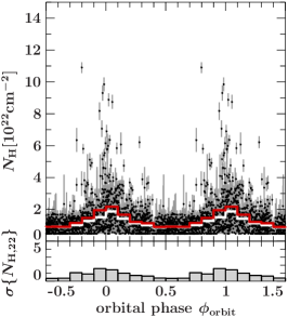
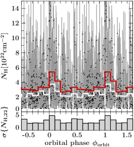
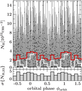
Figure 6: Variation of $N_{\mathrm{H}}$ with orbital phase for observations where the source was in the hard (left), intermediate (middle), and soft (right) state. The upper panels show the orbit dependence of $N_{\mathrm{H}}$ measurements for individual satellite orbit-wise spectra (black datapoints with gray uncertainties), as well as the average (red) and median (white) values for orbital phase bins with a width of $\Delta\phi_{\mathrm{orb}}=0.1$. The lower panels show the standard deviation $\sigma\{N_{\mathrm{H,22}}\}\coloneqq\sigma\{N_{\mathrm{H}}/(10^{22}\,\mathrm{cm}^{-2})\}$ of the $N_{\mathrm{H}}$ measurements. The panels specifically show 1515 hard state ($\Gamma_{1}\leq 2.0$) observations that do not require a disk component, 384 intermediate state ($2.0<\Gamma_{1}\leq 2.5$) observations that require a disk, and 506 soft state ($2.5<\Gamma_{1}$) observations (all soft state observations require a disk component).

When looking at the whole state-resolved sample, we determine the average and median values of $N_{\mathrm{H}}$ and its standard deviation, $\sigma\{N_{\mathrm{H,22}}\}\coloneqq\sigma\{N_{\mathrm{H}}/(10^{22}\,\mathrm{cm}^{-2})\}$, for phase bins of width $\Delta\phi_{\mathrm{orb}}=0.1$ starting at $\phi_{\mathrm{orb}}=0$. In the hard state, the average column values and the standard deviation, i.e., the variability of the wind between individual observations, increase around superior conjunction (Fig. 6, left).

Individual observations, especially for $\phi_{\mathrm{orb}}\sim 0$, show $N_{\mathrm{H}}$ values much larger than the average for a given phase (Fig. 6, left, see also Fig. 4 for example spectra). We associate these observations with the prolonged deep absorption events (often dubbed “dips”) known from the literature (Sect. 1) and carefully check our data to find out whether these observations have systematic differences to other observations in the same spectral state. We find no such differences; in particular, these “dips” do not have larger uncertainties in $N_{\mathrm{H}}$ and do not show clear trends in their exposure time, $\chi^{2}_{\mathrm{red}}$, unabsorbed 3–50 keV flux (see also Fig. 5), or the correlation between $\Gamma_{1}$ and $\Gamma_{2}$ known from Wilms et al. (2006). The dips cluster around superior conjunction, but individual strong absorption measurements occur as early as at $\phi_{\mathrm{orb}}\approx 0.8$ and as late as at $\phi_{\mathrm{orb}}\approx 0.3$ (Fig. 6, left).

The RXTE spectra do not allow a meaningful fit of partial covering models and so we cannot constrain possible partial covering either in physical space or in time (i.e., a clump or a group of clumps, possibly of different optical depth, passing through the line of sight for a part of the total exposure time of one spectrum). Thus, the $N_{\mathrm{H}}$-values derived for individual observations are lower limits on the sum of the absorption columns of individual clumps with the ISM absorption over a given observation’s exposure time (i.e., on average 1.6–1.7 ks, Fig. 1).

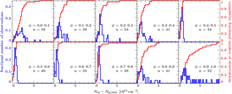
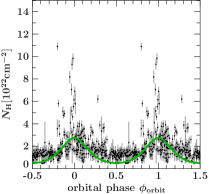
Figure 7: Observations from the hard state of 2006–2010 (MJD 53900–55375, Grinberg et al. 2013) that do not require a disk. Left: normalized histograms (blue) and normalized cumulative histograms (red) for $N_{\mathrm{H}}$ above the ISM value for individual orbital phase bins; $n$ denotes the total number of observations in a given orbital phase bin. Note that the phase bin $\phi=0.7\texttt{--}0.8$ contains one measurement in excess of $10^{23}\,\mathrm{cm}^{-2}$. Right: Orbital dependence of $N_{\mathrm{H}}$. The best fit focussed wind model introduced in Sect. 4.1.2 is shown in green.

Within the hard state, Cyg X-1 can display a range of spectral and timing behaviors (Pottschmidt et al. 2003; Wilms et al. 2006; Grinberg et al. 2014). At the same time, we expect the behavior of the absorption to depend on the broadband spectral shape of the X-ray source because of possible ionization of the wind. For a detailed analysis of absorption, we therefore need a hard state with stable spectral and timing characteristics, such as the long hard state of 2006–2010 (MJD 53900–55375, Grinberg et al. 2013, 2014). We show results for this long hard state period in Fig. 7; it includes 383 observations that do not require a disk (Fig. 2) and that have a total exposure time of 660 ks or $\sim$1.4 orbital periods of the system. The variability of absorption can be clearly seen in the (cumulative) probability distributions of $N_{\mathrm{H}}$ values at different orbital phases (Fig. 7, left). The values are low and the distribution narrow at $\phi_{\mathrm{orb}}\sim 0.5$. At $\phi_{\mathrm{orb}}\sim 0$, the distribution is broad with a higher average (average values and their standard deviations are shown in Fig. 9, right). We will use this set for comparisons with a toy model for the focussed wind and a clumpy wind model in Sect. 4.1.2 and 4.1.3, respectively.

3.2 Intermediate state and soft state

We now address observations of Cyg X-1 in the intermediate and the soft state, i.e., when the X-ray spectrum is much softer than in the hard state. Most data in the intermediate state require a disk component that leads to larger uncertainties in the $N_{\mathrm{H}}$ determination and particularly to a systematically increased average value independent of orbital phase as well as a larger $\sigma\{N_{\mathrm{H,22}}\}$. An increase of average $N_{\mathrm{H}}$ at $\phi_{\mathrm{orb}}\approx 0$ is, however, still visible (Fig. 6, middle).

Our data do not show orbital variability of absorption in the soft state (Fig. 6, right). The average values are comparable with the intermediate state, but in several phase bins we find median values of $4.8\times 10^{21}\,\mathrm{cm}^{-2}$, i.e., the data are consistent with no neutral absorption intrinsic to the source. Because of the increased disk contribution, observations in the soft state are even more affected by systematics than those in the intermediate state, especially given that the disk in Cyg X-1 has a temperature $\lesssim$0.4 keV ($\approx 4.6\times 10^{6}$ K) even in the soft state (Wilms et al. 2006, and our fits), i.e., it peaks below the lower limit of our data so that the disk parameters show relatively large uncertainties.

4 Discussion

4.1 Hard state

4.1.1 Discussion and comparison to earlier results

Our results show that despite PCA’s energy coverage only above $\sim$3 keV and comparatively low spectral resolution when compared to CCD or even grating instruments, PCA data can be used to assess trends in the behavior of the absorption. The changes in $N_{\mathrm{H}}$ strongly influence the shape of the observed spectra (Fig. 4). The overall orbital variability of $N_{\mathrm{H}}$ values found here is consistent with earlier results (Feng & Cui 2002; Ibragimov et al. 2005; Wilms et al. 2006; Boroson & Vrtilek 2010). To our knowledge, we are the first to quantify the variance of the equivalent hydrogen column, $\sigma\{N_{\mathrm{H,22}}\}$ (Fig. 6, lower panels).

The largest $N_{\mathrm{H}}$ values seen during the hard state (Figs. 4 and 7) are on the order of $10^{23}\,\mathrm{cm}^{-2}$. Kitamoto et al. (1984, using Tenma), Bałucińska-Church et al. (1997, using ASCA), and Hanke et al. (2008, using Chandra) reported individual deep absorption events with $N_{\mathrm{H}}\gtrsim 10^{23}\,\mathrm{cm}^{-2}$. Periods of increased absorption that lasted longer than a few ks have been observed with various instruments, especially close to superior conjunction. For example, Feng & Cui (2002) discuss a long dip of at least $\sim$3 ks that shows complex substructure. Prolonged periods of increased absorption are also clearly seen in the long uninterrupted observations possible with Chandra (Hanke et al. 2008). Given these previous measurements and the size of our sample, the detection of several strong absorption events as discussed in Sect. 3.1 is plausible.

Bałucińska-Church et al. (2000) have used mainly RXTE-All Sky Monitor (ASM; Levine et al. 1996) data to show orbital variability in ASM-based hardness ratios and in dip (defined by a threshold ASM hardness ratio) occurrence, both peaking at superior conjunction consistent with the behavior of the absorption column density that we observe. They observe a peak in the dip occurence at $\phi_{\mathrm{orb}}=0.95$, but our sample is not large enough to track this possible assymetry of the $N_{\mathrm{H}}$ distribution around $\phi_{\mathrm{orb}}=0$. Poutanen et al. (2008) further show that the orbital modulation of ASM countrates in the hard state depends on the superorbital phase: the number of ASM-defined dips shows a superorbital periodicity when assuming a $\sim$150 d superorbital period. The smaller number of our measurements when compared to ASM data combined with the apparent stochastic nature and large variance of the absorption variations do not allow such an analysis here.

Despite these shortcomings, the exceptional coverage of the pointed observation allows us to compare the observational results to theoretical models. In particular we quantitatively compare a simple focussed CAK wind to our data from the stable hard state period of 2006–2010 ($\sim$250 orbits of the binary system) in Sect. 4.1.2, and, for the first time for a high mass black hole binary, qualitatively match the observed data from the same stable hard state period with predictions from a clumpy wind model for O-star winds in Sect. 4.1.3.

4.1.2 Focussed wind model in the hard state

We first compare the orbital variation of $N_{\mathrm{H}}$ from MJD 53900–55370 with a toy model for the focussed wind as introduced by Gies & Bolton (1986b). This model is based on the previous work of Friend & Castor (1982) and depends on the angle $\theta$ between the wind direction and the donor-black hole axis. We emphasize that this is only a toy model that does not take into account details of both the physics of a real wind and the observations used. The model is, however, useful to assess general trends and to point out the directions in which better models have to be developed.

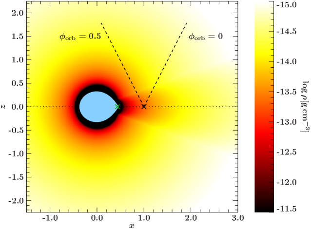
Figure 8: Stellar wind density calculated following the focussed wind model of Gies & Bolton (1986a). The $x$- and $z$- axes are shown in units of orbital separation. The position of the black hole is marked with a black cross, the position of the center of mass with a green cross. Lines of sight towards the black hole at orbital phases 0 and 0.5 are indicated by dashed lines, the orbital plane by a dotted line. Note that there are no discotinuities in the wind; if such appear above, they are unfortunate tricks of vision.

For $\theta\geqq 20^{\circ}$, the wind is the radiatively driven (CAK-)wind of a single star (Castor et al. 1975). For $\theta<20^{\circ}$, the wind varies smoothly with $\theta$ with terminal velocity and density peaking at $\theta=0$. In particular, we employ the model with the fill-out-factor of 0.98 with the correspondent values for terminal velocity and wind density listed in Table 1 of Gies & Bolton (1986a) and use masses, inclination, and orbital period as given in Sect. 1. Figure  8 shows the resulting distribution of wind density.

We obtain the total (neutral and ionized) column density by integrating along the line of sight towards the black hole at a given orbital phase: these values are on the order of 3–$5\times 10^{22}\mathrm{cm}^{-2}$, i.e., much higher than the measured average values and more reminiscent of dips (cf. Fig. 6, left) But this total column density is not the $N_{\mathrm{H}}$ measured in our observations: the fully ionized part of the wind is transparent to X-rays and thus only some weakly to moderately ionized part of the wind will contribute to the measured absorption. We can hence assume that the absorption in the binary is restricted to the region of the wind with $\log\xi<\log\xi_{\mathrm{max}}$ with the ionization parameter $\xi$ defined after Tarter et al. (1969) as $\xi=L/(nr^{2})$ with $n$ being the absorbing particle number density, $r$ the distance from the ionizing source, and $L$ the luminosity above the hydrogen Lyman edge (typical for Cyg X-1: $L=10^{37}\,\mathrm{erg}\,\mathrm{s}^{-1}$, Miškovičová et al. 2015). We then consider only the contribution of those parts of the wind that satisfy this condition.

We take into account the ISM column density $N_{\mathrm{H,ISM}}$ and fit the parameter $\log\xi_{\mathrm{max}}$ of this model to the data. We obtain $\log\xi_{\mathrm{max}}\approx 2.7$, however with $\chi^{2}_{\mathrm{red}}=9.1$ for 382 degrees of freedom. The phase variation of $N_{\mathrm{H}}$ that corresponds to our best fit value of $\log\xi_{\mathrm{max}}$ is shown in Fig. 7, right panel, as a green curve. The failure to describe the data well is expected since the toy model does not include clumping that we expect to majorly contribute to the spread of the $N_{\mathrm{H}}$ measurements at a given orbital phase. To conduct a simple test for the influence of clumping on our results, we remove the 13 measurements with $N_{\mathrm{H}}>5\times 10^{22}\,\mathrm{cm}^{-2}$ and obtain a bestfit $\chi^{2}_{\mathrm{red}}=4.5$ for 369 degrees of freedom with a decreased bestfit value ($\log\xi_{\mathrm{max}}\approx 2.67$ as compared to previously $\log\xi_{\mathrm{max}}\approx 2.71$).

The toy model also neglects additional smaller effects such as a potential photoionization wake that would introduce asymmetries (Blondin 1994). Uncertainties in determination of the ISM absorption, $N_{\mathrm{H,ISM}}$, towards the source may lead to further problems (Xiang et al. 2011). However, it is interesting to note that when we account for the fact that our measurements include the clumping, our result is in rough agreement with results ($\log\xi\lesssim 2.6$) found by Miškovičová et al. (2015), who infer $N_{\mathrm{H}}$ values ranging from $6.8\times 10^{21}\,\mathrm{cm}^{-2}$ to $1.3\times 10^{22}\,\mathrm{cm}^{-2}$ from modelling the Ne edge in the non-dip parts of hard state Chandra observations at 5 different orbital phases.

4.1.3 Clumpy wind model for the hard state

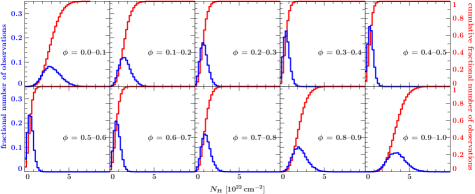
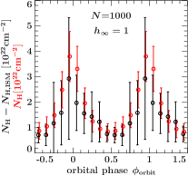
Figure 9: Predictions of $N_{\mathrm{H}}$ variability assuming a clumpy wind model with the total number of clumps per flow time $N=1000$ and the terminal porosity length $h_{\infty}=R_{*}$ (see Sect. 4.1.3 for explanation of parameters). Left: model histograms for the distribution of equivalent absorption column density $N_{\mathrm{H}}$. Right: average values (circles) and standard deviations (‘error bars’ on the average values) in a given orbital phase for the theoretical model (red) and values measured in the hard state of MJD 53900-55375 (black). Average measured values are shown as ‘$\mbox{average}-N_{\mathrm{H,ISM}}$’ to account for the ISM absorption.

We next consider whether the observed variability in absorbing column could be due to wind structures, and how the characteristics of those structures compare to what is known about radiatively driven winds in other contexts, such as clumps (Abbott et al. 1981; Hillier & Miller 1998; Fullerton et al. 2006; Puls et al. 2006) or discrete absorption components (DACs; Prinja & Howarth 1986). To this end, we use a numerical code to simulate the column density between the observer and a point-like X-ray source, as the source orbits around a companion whose wind is composed of discrete clumps. For simplicity, the code does not account for the focussed wind properties of the system; moreover, the clumps are assumed to be spherical, rather than the pancake morphologies considered by other authors (e.g., Feldmeier et al. 2003; Oskinova et al. 2004). At a given orbital phase, the column-density evaluation is performed by casting a ray from the source to the observer, determining which ray segments lie inside clumps, and summing up the contributions from these segments (as the product of the segment length and the clump density).

The distribution of clumps throughout the wind follows a similar approach to that described in Appendix A of Sundqvist et al. (2012). Clumps are relased at the stellar surface $r=R_{*}$ in a random direction and with an initial radial size $l_{*}$, and then advect outward with the wind according to a canonical ‘$\beta$’ velocity law $\varv(r)=\varv_{\infty}(1-R_{*}/r)^{\beta}$. As a clump advects its radial size grows as $l(r)=(r/R_{*})l_{*}$, but its mass remains fixed at $m=\dot{M}/\dot{N}$ where $\dot{M}$ is the overall wind mass loss rate, and $\dot{N}$ is the clump release rate. The latter is most conveniently parameterized in terms of the number of clumps per wind flow time $N=\dot{N}t_{\rm flow}$, with $t_{\rm flow}\equiv R_{*}/\varv_{\infty}$. To relate these parameters to the porosity length $h$ (essentially, the mean free path between clumps; see Owocki & Cohen 2006), we note that $h(r)=h_{\infty}\varv(r)/\varv_{\infty}$, where the terminal porisity length is

$$h_{\infty}\equiv 3\frac{R_{*}}{l_{*}^{2}N}.$$ (1)

To apply the code to Cyg X-1, we assume $\beta=1.6$, $R_{*}=18\,R_{\odot}$, $\varv_{\infty}=2400\,{\rm km\,s^{-1}}$, and $\dot{M}=2\times 10^{-6}\,{\rm M_{\odot}\,yr^{-1}}$, and adopt the orbital parameters given in Section 1. We ran a grid of simulations with $N=100,316,1000,3162$ and 10000, and $h_{\infty}/R_{*}=0.1,0.316,1,3.162$, and 10 to explore the level of variability expected on the time scales we probe here. For each grid point we calculated 1000 model orbits, with a phase resolution $\Delta\phi_{\mathrm{orb}}=0.001$. Since typical RXTE observations of Cyg X-1 had an exposure of about 0.005 orbits, and since each observation is not subdivided into time slices, it is necessary to average the model to a timescale corresponding to the observations. Thus, we rebinned the models by a factor of five by taking a linear average of the model column density. A linear average over a phase bin does not strictly correctly account for the non-linear addition of partial covering in time, but is adequate given the crude nature of our model. Likewise, rebinning by a factor of five is not an exact match to the actual observations, but it is an adequate approximation.

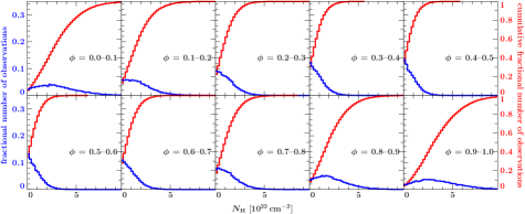
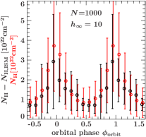
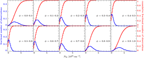
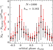
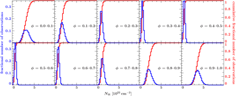
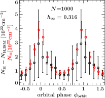
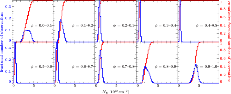
Figure 10: Predictions of $N_{\mathrm{H}}$ variability assuming a clumpy wind model with the total number of clumps per flow time $N=1000$ and varying terminal porosity length $h_{\infty}=10$, 3.162, 0.316, and 0.1$R_{*}$ (see Sect. 4.1.3 for explanation of parameters and Fig. 9 for the case of $h_{\infty}=1$). Left: model histograms for the distribution of equivalent absorption column density $N_{\mathrm{H}}$. Right: average values (circles) and standard deviations (‘error bars’ on the average values) in a given orbital phase for the theoretical model (red) and values measured in the hard state of MJD 53900-55375 (black). Average measured values are shown as ‘$\mbox{average}-N_{\mathrm{H,ISM}}$’ to account for the ISM absorption.

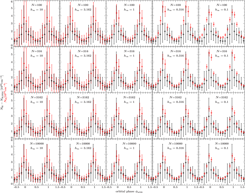
Figure 11: Predictions of $N_{\mathrm{H}}$ variability assuming a clumpy wind model with the total number of clumps per flow time $N$ and varying terminal porosity length $h_{\infty}$. Shown are average values (circles) and standard deviations (‘error bars’ on the average values) in a given orbital phase for the theoretical model (red) and values measured in the hard state of MJD 53900-55375 (black). Average measured values are shown as ‘$\mbox{average}-N_{\mathrm{H,ISM}}$’ to account for the ISM absorption. For the case of $N=1000$ see Figs. 9 and  10.

The statistical properties of each phase bin of 0.005 orbits do not change rapidly as a function of orbital phase, so these statistical properties were further averaged into phase bins of 0.1 orbits, corresponding to the grouping used to evaluate the observations. We show this statistical analysis of the column for $N=1000$ and $h_{\infty}=R_{*}$ in Fig. 9; the mean and standard deviation of this model are compared to those of the data in the right panel. We have chosen a model with a similar level of variability as the observations near phase 0.5, where our line of sight to the compact object mainly probes the part of the wind that is likely least perturbed by the peculiarities of the focussed part of the wind. For other model realizations see Figs. 10 and 11.

The choice of porosity length $h_{\infty}$ has a strong effect in determining the level of variability in the model (Fig. 10). The choice of $N$ has a weaker effect, with larger values of $N$ (and thus small values of $l_{*}$) showing somewhat reduced variability (Fig. 11). This is a result of single observations averaging over the transit of one or more clumps across the line of sight, thus washing out the variability expected on short timescales. We have explored the effect of different choices of averaging timescale (or equivalently observation duration) in our simulations, and as expected, we find that increasing the averaging timescale tends to reduce the variability (see also Sect. 3.1 for a discussion of exposure times on the measured $N_{\mathrm{H}}$). We also find that there is a maximum useful time resolution above which increasing the sampling rate does not increase the level of variability observed. This maximum rate corresponds roughly to the time scale for a typical clump to transit our line of sight to the compact object which is on the order of $l_{*}/\varv_{\infty}$ (when the wind velocity dominates over orbital velocity as is the case here). One obvious conclusion of these results is that the clump size scale could be constrained by obtaining spectra of high statistical quality (e.g., with Suzaku or Chandra satellites) and exploring the level of variability on shorter time scales.

The models with $h_{\infty}=R_{*}$ have the best agreement with the data near $\phi_{\mathrm{orb}}=0.5$, with the exception that for $N=10000$ the model with $h_{\infty}=3.162R_{*}$ has the best agreement (Fig. 11). Based on previous theoretical and observational investigations of single O stars, it is reasonable that $h_{\infty}$ should be comparable to or smaller than $R_{*}$ (Dessart & Owocki 2003; Owocki & Cohen 2006; Nazé et al. 2013). This is also consistent with the results of Leutenegger et al. (2013), who found that the spectrum of the single O supergiant $\zeta$ Pup could be fit with models having porosity lengths $h_{\infty}\leq R_{*}$. To test for the influence of terminal velocity on our results, we re-ran the simulations with $\varv_{\infty}=1600\,\mathrm{km}\,\mathrm{s}^{-1}$. Although the resulting mean values for $N_{\mathrm{H}}$ are higher (due to the increased wind density), our results are otherwise similar to the original $\varv_{\infty}=2400\,\mathrm{km}\,\mathrm{s}^{-1}$ grid, and thus our conclusions do not change.

Comparing Fig. 7 and 9, the model shows a Gaussian distribution of absorbing columns, while the data show a non-Gaussian tail near phase 0. It seems likely that this non-Gaussian tail reflects some unusual wind structure related to the focussed wind. However, since the impact parameter of our line of sight with respect to the optical companion is smallest near this orbital phase, the tail might also be a signature of a wind with pancake-shaped clumps, which would be effectively more porous when viewed edge on (Feldmeier et al. 2003; Oskinova et al. 2012). A more thorough exploration of these effects may give insight into their importance but it is beyond the scope of this paper.

4.2 Intermediate state and soft state

Due to the lack of suitable observations in the previously analyzed samples, the variability of absorption in intermediate and soft states has not been previously analyzed using RXTE spectra, but only using ASM data. Boroson & Vrtilek (2010) analyzed orbital variability of absorption in five soft state periods. Boroson & Vrtilek see no variability in their soft states 2 and 5 that would be mostly classified as intermediate states using the more rigorous state definitions of Grinberg et al. (2013). Their soft state 3 shows orbital variability. Boroson & Vrtilek (2010) also point out that the intrinsic variability of the X-ray source in the softer periods hampers the search for periodicities in ASM data.

Based on the pointed RXTE data alone, we see no orbital variability in the soft state, while there are signs for an increase of the main absorption toward $\phi_{\mathrm{orb}}\approx 0$ in the intermediate state. These results qualitatively agree with the behavior seen in analyses of Chandra high resolution spectra: as the source softens, dipping becomes less pronounced (Miškovičová et al. 2015). However, dips have still been observed in the soft state with Suzaku (Yamada et al. 2013, but note the strong changes in hardness ratio in their data that may be indicative of spectral evolution during the observation). Hanke (2011) shows lightcurves and softness ratios of all Chandra observations up to and including ObsID 13219 taken in 2011 February: some weak and short dipping can be seen in the soft state data.

The interpretation of these results in the context of the previous Suzaku and Chandra results is that the soft X-rays emitted from the vicinity of the black hole in the soft state are strong enough to fully ionize the wind and even some or all of the optically thick clumps. The wind thus becomes (mainly) transparent to X-rays and no orbital variation of absorption column can be seen.

5 Summary and conclusions

We have analyzed almost 5 Ms of RXTE observations of Cyg X-1 taken over a span of 16 years in different spectral states. We find clear orbital variability of absorption in the hard state of the X-ray source with an overall increase and additional deep absorption events (“dips” with $N_{\mathrm{H}}\sim 10^{23}\mathrm{cm}^{-2}$) around superior conjunction, in agreement with previous work with different instruments. Because of the presence of an additional multitemperature disk component in the spectra, the absorption column cannot be well constrained in the intermediate and soft states. However, there are signs for increased $N_{\mathrm{H}}$ towards $\phi_{\mathrm{orb}}=0$ in the intermediate state.

We compared the observed orbital variability of absorption with two wind models. A toy model for a focussed line-driven wind without clumps (Gies & Bolton 1986b) does not describe the data well and we attribute the differences to the absence of clumping in the model that would lead to the observed strong variations of $N_{\mathrm{H}}$ at the same orbital phase. Qualitatively matching the observed $N_{\mathrm{H}}$ distributions at a given orbital phase to a toy clumpy wind model (Owocki & Cohen 2006; Sundqvist et al. 2012) without a focussed wind and with spherical clumps results in the best match for models with porosity length, $h_{\infty}$, on the order of the stellar radius, $R_{*}$, at orbital phases $\phi_{\mathrm{orb}}\approx 0.5$, in agreement with results from (effectively) single O stars (Leutenegger et al. 2013). Our models exclude both much lower and much higher porosities. The discrepancies between the toy clumpy wind model and data at $\phi_{\mathrm{orb}}\approx 0$ could be due to either a focussed wind component or a non-spherical shape of the clumps or a combination of both. We note here that the existence of a focussed wind component in Cyg X-1 is supported by multiple lines of evidence such as optical measurements (Gies & Bolton 1986b; Sowers et al. 1998).

While we caution against an over-interpretation of details of the presented simple models they firstly demonstate that RXTE data of Cyg X-1 can indeed be used for an analysis of the long-term orbital variability of absorption and secondly clearly demand better models. In particular, a thorough exploration of the winds will require a model that includes both, the focussed and the clumpy structure of the wind, and possibly also different clump shapes and/or sizes.

Appendix A Clumpy wind model simulations