Effects of applied fields on quantum coupled double-well systems

Abstract

Effects of time-dependent applied fields on quantum coupled double-well (DW) systems with Razavy’s hyperbolic potential have been studied. By solving the Schrödinger equation for the DW system, we have obtained time-dependent occupation probabilities of the eigenstates, from which expectation values of positions $x_{1}$ and $x_{2}$ of particles ($\langle x_{1}+x_{2}\rangle$), the correlation ($\Gamma(t)$) and the concurrence ($C(t)$) expressing a degree of the entanglement of the coupled DW system, are obtained. Analytical expressions for $\langle x_{1}+x_{2}\rangle$, $\Gamma(t)$ and $C(t)$ are derived with the use of the rotating-wave approximation (RWA) for sinusoidal fields. Model calculations have indicated that $\langle x_{1}+x_{2}\rangle$, $\Gamma(t)$ and $C(t)$ show very complicated time dependences. Results of the RWA are in good agreement with exact ones evaluated by numerical methods for cases of weak couplings and small applied fields in the near-resonant condition. Applications of our method to step fields are also studied.

Keywords: coupled double-well potential, Razavy’s potential, rotating-wave approximation, entanglement

I Introduction

Extensive studies have been made for quantum double-well (DW) systems in physics and chemistry where a tunneling is one of intrigue quantum phenomena Tannor07 . Effects of applied fields on DW systems have been studied (for review see Grifoni98 ). Various phenomena such as a coherent destruction of tunneling by applied fields were pointed out Grossmann91 . The two-level (TL) system which is a simplified model of a DW system, has been employed for a study on qubits which play important roles in quantum information and quantum computation. Many theoretical studies on effects of fields applied to single and coupled qubits have been reported with the use of the TL model Storcz01 ; Satanin12 ; Bina14 ; Pal14 . In contrast to the simplified TL model, studies on coupled DW systems which are commonly described by the quartic potentials are scanty Gupta06 , because a calculation of such a system is much tedious than that of the coupled TL model, even for the absence of applied fields. One of difficulties in studying coupled DW systems is that one cannot obtain exact eigenvalues and eigenfunctions of the Schrödinger equation for quartic DW potential. Then one has to apply various approximate approaches such as perturbation and spectral methods to quartic DW models. Razavy Razavy80 proposed quasi-exactly solvable hyperbolic DW potential for which one may exactly determine a part of whole eigenvalues and eigenfunctions. A family of quasi-exactly solvable potentials has been investigated Finkel99 ; Bagchi03 .

Recently the present author Hasegawa15 has investigated the relation between the entanglement and the speed of evolution in coupled DW system described by Razavy’s potential. It would be interesting to study effects of applied fields on coupled DW systems with Razavy’s potential, which is the purpose of the present study. Some sophisticated methods like the Floquet approach have been developed in solving Schrödinger equation for time-dependent periodic fields. In order to treat the periodic as well as non-periodic dynamical fields, we solve in this study the time-dependent Schrödinger equation by a straightforward method. An advantage of our approach is that we may exactly determine eigenvalues and eigenfunctions of driven coupled DW systems. We calculate expectation values of various quantities such as positions of particles, the correlation and the concurrence which expresses a measure of the entanglement of a coupled DW system. Effects of applied fields are analytically studied with the use of the rotating-wave approximation (RWA) which has been widely adopted for sinusoidal periodic field, in particular for the TL model. The validity of the RWA may be examined by a comparison between results of the RWA and exact ones evaluated by numerical methods.

The paper is organized as follows. In Sec. II, the calculation method employed in our study is explained with a brief review on Razavy’s hyperbolic potential Razavy80 . Equations of motion for populations of four energy levels are obtained from the time-dependent Schrödinger equation of driven coupled DW systems. Expressions for expectation values of particle positions, the correlation and the concurrence are calculated. For sinusoidal fields, we present their analytical expressions by using the RWA. In Sec. III, we report model calculations with the use of the RWA and numerical methods when the sinusoidal fields are applied to the initial ground state. In Sec. IV, calculations are made for sinusoidal fields applied to the initially wavepacket state. Our method is applied also to the case of applied step fields. Sec. V is devoted to our conclusion.

II Coupled double-well system with Razavy’s potential

II.1 Calculation method

We consider coupled two DW systems whose Hamiltonian is given by

$$H = H_{0}+H_{C}+H_{I},$$ (1)

where

$$H_{0} = \sum_{n=1}^{2}\left[-\frac{\hbar^{2}}{2m}\frac{\partial^{2}}{\partial x_{n}^{2}}+V(x_{n})\right],$$ (2)

$$H_{C} = -gx_{1}x_{2},$$ (3)

$$H_{I} = -(x_{1}+x_{2})F(t),$$ (4)

$$V(x) = \frac{\hbar^{2}}{2m}\left[\frac{\xi^{2}}{8}\>{\rm cosh}\>4x-4\xi\>{\rm cosh}\>2x-\frac{\xi^{2}}{8}\right].$$ (5)

Here $x_{1}$ and $x_{2}$ stand for coordinates of two distinguishable particles of mass $m$, $H_{0}$ signifies a DW system with Razavy’s potential $V(x)$ Razavy80 , $H_{C}$ means the coupling term with an interaction $g$, and $H_{I}$ includes the time-dependent applied field $F(t)$ whose explicit form will be given shortly [Eq. (53) or (101)]. The case of $H_{I}$ which is more general than Eq. (4) will be studied in the Appendix. The potential $V(x)$ with $\hbar=m=\xi=1.0$ adopted in this study is plotted in Fig. 1(a). Minima of $V(x)$ locate at $x_{s}=\pm 1.38433$ with $V(x_{s})=-8.125$ and its maximum is $V(x)=-2.0$ at $x=0.0$.

Firstly we consider only $H_{0}$ in Eq. (2), whose eigenvalues are given Razavy80

$$\epsilon_{0} = \frac{\hbar^{2}}{2m}\left[-\xi-5-2\sqrt{4-2\xi+\xi^{2}}\right],$$ (6)

$$\epsilon_{1} = \frac{\hbar^{2}}{2m}\left[\xi-5-2\sqrt{4+2\xi+\xi^{2}}\right],$$ (7)

$$\epsilon_{2} = \frac{\hbar^{2}}{2m}\left[-\xi-5+2\sqrt{4-2\xi+\xi^{2}}\right],$$ (8)

$$\epsilon_{3} = \frac{\hbar^{2}}{2m}\left[\xi-5+2\sqrt{4+2\xi+\xi^{2}}\right],$$ (9)

and whose eigenfunctions are given by

$$\phi_{0}(x) = A_{0}\;e^{-\xi\>{\rm cosh}\>2x/4}\left[3\xi\>{\rm cosh}\>x+(4-\xi+2\sqrt{4-2\xi+\xi^{2}})\>{\rm cosh}\>3x\right],$$ (10)

$$\phi_{1}(x) = A_{1}\;e^{-\xi\>{\rm cosh}\>2x/4}\left[3\xi\>{\rm sinh}\>x+(4+\xi+2\sqrt{4+2\xi+\xi^{2}})\>{\rm sinh}\>3x\right],$$ (11)

$$\phi_{2}(x) = A_{2}\;e^{-\xi\>{\rm cosh}\>2x/4}\left[3\xi\>{\rm cosh}\>x+(4-\xi-2\sqrt{4-2\xi+\xi^{2}})\>{\rm cosh}\>3x\right],$$ (12)

$$\phi_{3}(x) = A_{3}\;e^{-\xi\>{\rm cosh}\>2x/4}\left[3\xi\>{\rm sinh}\>x+(4+\xi-2\sqrt{4+2\xi+\xi^{2}})\>{\rm sinh}\>3x\right],$$ (13)

$A_{n}$ ($n=0,1$) denoting normalization factors. Eigenvalues for the adopted parameters are $\epsilon_{0}=-4.73205$, $\epsilon_{1}=-4.64575$, $\epsilon_{2}=-1.26795$ and $\epsilon_{3}=0.645751$. Both $\epsilon_{0}$ and $\epsilon_{1}$ locate below $V(0)$ as shown by dashed curves in Fig. 1(a), and $\epsilon_{2}$ and $\epsilon_{3}$ are far above $\epsilon_{1}$. In this study, we take into account only the lowest two states with $\epsilon_{0}$ and $\epsilon_{1}$, which is justified because of $\epsilon_{1}-\epsilon_{0}$ ($=0.0863$) $\ll\epsilon_{2}-\epsilon_{1}$ ($=3.3778$). Figure 1(b) shows eigenfunctions of $\phi_{0}(x)$ and $\phi_{1}(x)$, which are symmetric and anti-symmetric, respectively, with respect to the origin.

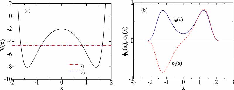
Figure 1: (Color online) (a) Razavy’s DW potential $V(x)$ (solid curve), dashed and chain curves expressing eigenvalues of $\epsilon_{0}$ and $\epsilon_{1}$, respectively, for $\hbar=m=\xi=1.0$ [Eq.(5)]. (b) Eigenfunctions of $\phi_{0}(x)$ (solid curve) and $\phi_{1}(x)$ (dashed curve).

Secondly we include the coupling term $H_{C}$ in Eq. (3). With basis states of $\phi_{0}(x_{1})\phi_{0}(x_{2})$, $\phi_{0}(x_{1})\phi_{1}(x_{2})$, $\phi_{1}(x_{1})\phi_{0}(x_{2})$ and $\phi_{1}(x_{1})\phi_{1}(x_{2})$, the energy matrix of the Hamiltonian of $H_{0}+H_{C}$ is expressed by

$${\cal H}_{0}+{\cal H}_{C} = \left({\begin{array}[]{*{20}c}{2\epsilon_{0}}&{0}&{0}&{-g\gamma^{2}}\\ {0}&{\epsilon_{0}+\epsilon_{1}}&{-g\gamma^{2}}&{0}\\ {0}&{-g\gamma^{2}}&{\epsilon_{0}+\epsilon_{1}}&{0}\\ {-g\gamma^{2}}&{0}&{0}&{2\epsilon_{1}}\\ \end{array}}\right),$$ (18)

with

$$\gamma = \int_{-\infty}^{\infty}\phi_{0}(x)\>x\>\phi_{1}(x)\>dx=1.13823.$$ (19)

Eigenvalues of the energy matrix of ${\cal H}_{0}+{\cal H}_{C}$ are given by

$$E_{0} = \epsilon-\sqrt{\delta^{2}+g^{2}\gamma^{4}},$$ (20)

$$E_{1} = \epsilon-g\gamma^{2},$$ (21)

$$E_{2} = \epsilon+g\gamma^{2},$$ (22)

$$E_{3} = \epsilon+\sqrt{\delta^{2}+^{2}\gamma^{4}},$$ (23)

where

$$\epsilon = \epsilon_{1}+\epsilon_{0}=-9.3778,$$ (24)

$$\delta = \epsilon_{1}-\epsilon_{0}=0.0863.$$ (25)

Corresponding eigenfunctions are given by

$$\Phi_{0}(x_{1},x_{2}) = \cos\theta\>\phi_{0}(x_{1})\phi_{0}(x_{2})+\sin\theta\>\phi_{1}(x_{1})\phi_{1}(x_{2}),$$ (26)

$$\Phi_{1}(x_{1},x_{2}) = \frac{1}{\sqrt{2}}\left[\phi_{0}(x_{1})\phi_{1}(x_{2})+\phi_{1}(x_{1})\phi_{0}(x_{2})\right],$$ (27)

$$\Phi_{2}(x_{1},x_{2}) = \frac{1}{\sqrt{2}}\left[-\phi_{0}(x_{1})\phi_{1}(x_{2})+\phi_{1}(x_{1})\phi_{0}(x_{2})\right],$$ (28)

$$\Phi_{3}(x_{1},x_{2}) = -\sin\theta\>\phi_{0}(x_{1})\phi_{0}(x_{2})+\cos\theta\>\phi_{1}(x_{1})\phi_{1}(x_{2}),$$ (29)

where

$$\tan\>2\theta = \frac{g\gamma^{2}}{\delta}.\;\;\;\;\mbox{$\left(-\frac{\pi}{4}\leq\theta\leq\frac{\pi}{4}\right)$}$$ (30)

We hereafter assume $g\geq 0$ Hasegawa15 . The $g$ dependence of $E_{\nu}$ ($\nu=0-3$) is shown in Fig. 2 of Ref. Hasegawa15 .

Thirdly we take into account $H_{I}$ for an applied field in Eq. (4). The energy matrix of the time-dependent total Hamiltonian $H$ ($=H_{0}+H_{C}+H_{I}$) with basis states of $\phi_{0}(x_{1})\phi_{0}(x_{2})$, $\phi_{0}(x_{1})\phi_{1}(x_{2})$, $\phi_{1}(x_{1})\phi_{0}(x_{2})$ and $\phi_{1}(x_{1})\phi_{1}(x_{2})$ is expressed by

$${\cal H}_{0}+{\cal H}_{C}+{\cal H}_{I} = \left({\begin{array}[]{*{20}c}{2\epsilon_{0}}&{-\gamma F(t)}&{-\gamma F(t)}&{-g\gamma^{2}}\\ {-\gamma F(t)}&{\epsilon_{0}+\epsilon_{1}}&{-g\gamma^{2}}&{-\gamma F(t)}\\ {-\gamma F(t)}&{-g\gamma^{2}}&{\epsilon_{0}+\epsilon_{1}}&{-\gamma F(t)}\\ {-g\gamma^{2}}&{-\gamma F(t)}&{-\gamma F(t)}&{2\epsilon_{1}}\\ \end{array}}\right).$$ (35)

Alternatively, the energy matrix of $H$ may be expressed with basis states of $\Phi_{0}$, $\Phi_{1}$, $\Phi_{2}$ and $\Phi_{3}$ in Eqs. (26)-(29) by

$${\cal H} = \left({\begin{array}[]{*{20}c}{E_{0}}&{-\alpha F(t)}&{0}&{0}\\ {-\alpha F(t)}&{E_{1}}&{0}&{-\beta F(t)}\\ {0}&{0}&{\;\;E_{2}}&{0}\\ {0}&{-\beta F(t)}&{0}&{E_{3}}\\ \end{array}}\right),$$ (40)

where

$$\alpha = \sqrt{2}\gamma(\cos\theta+\sin\theta),$$ (42)

$$\beta = \sqrt{2}\gamma(\cos\theta-\sin\theta).$$ (43)

In our following analysis, we adopt the energy matrix given by Eq. (LABEL:eq:A12) because it has more transparent physical meaning than Eq. (35). We expand the eigenstate $\Psi(x_{1},x_{2},t)$ of $H$ in terms of $\Phi_{\nu}(x_{1},x_{2})$ ($\nu=0-3$) with the time-dependent expansion coefficients $a_{\nu}(t)$ as

$$\Psi(t) = \Psi(x_{1},x_{2},t)=\sum_{\nu=0}^{3}\>a_{\nu}(t)\>\Phi_{\nu}(x_{1},x_{2})\>e^{-iE_{\nu}t/\hbar},$$ (44)

where expansion coefficients satisfy the relation

$$\sum_{\nu=0}^{3}|a_{\nu}(t)|^{2} = 1.$$ (45)

The Schrödinger equation: $i\hbar\>d\Psi(t)/dt=H\psi(t)$ becomes

$$i\hbar\sum_{\nu=0}^{3}\frac{d}{dt}\left[a_{\nu}(t)\Phi_{\nu}\>e^{-iE_{\nu}t/\hbar}\right]=\sum_{\nu=0}^{3}a_{\nu}(t)E_{\nu}\Phi_{\nu}\>e^{-iE_{\nu}t/\hbar}+\sum_{\nu=0}^{3}a_{\nu}(t)H_{I}\Phi_{\nu}\>e^{-iE_{\nu}t/\hbar}.$$ (46)

Multiplying $\Phi^{*}_{\mu}$ $(\mu=0-3)$ from the left side of Eq. (46) and integrating it over $x_{1}$ and $x_{2}$, we obtain equations of motion for $a_{\mu}(t)$

$$i\hbar\>\frac{da_{\mu}(t)}{dt} = \sum_{\nu=0}^{3}\langle\Phi_{\mu}|H_{I}|\Phi_{\nu}\rangle\>e^{-i\Delta_{\nu\mu}t}\>a_{\nu}(t),\hskip 28.45274pt\mbox{ $(\mu=0-3)$}$$ (47)

where

$$\Delta_{\nu\mu} = \frac{E_{\nu}-E_{\mu}}{\hbar}.$$ (48)

With the use of the energy matrix in Eq. (LABEL:eq:A12), equations of motion for $a_{\mu}(t)$ become [the argument $t$ in $a_{\nu}(t)$ is hereafter suppressed]

$$i\hbar\>\frac{da_{0}}{dt} = -\alpha F(t)\>e^{-i\Delta_{10}t}a_{1},$$ (49)

$$i\hbar\>\frac{da_{1}}{dt} = -\alpha F(t)\>e^{i\Delta_{10}t}a_{0}-\beta F(t)e^{-i\Delta_{31}t}a_{3},$$ (50)

$$i\hbar\>\frac{da_{2}}{dt} = 0,$$ (51)

$$i\hbar\>\frac{da_{3}}{dt} = -\beta F(t)\>e^{i\Delta_{31}t}a_{1}.$$ (52)

When we apply the sinusoidal field given by

$$F(t) = f\>\sin\>\omega t,$$ (53)

Eqs. (49)-(52) become

$$\frac{da_{0}}{dt} = \left(\frac{\alpha f}{2\hbar}\right)\left[e^{i(\omega-\Delta_{10})t}-e^{-i(\omega+\Delta_{10})t}\right]\>a_{1},$$ (54)

$$\frac{da_{1}}{dt} = \left(\frac{\alpha f}{2\hbar}\right)\left[e^{-(\omega+\Delta_{10})t}-e^{-i(\omega-\Delta_{10})t}\right]\>a_{0}+\left(\frac{\beta f}{2\hbar}\right)\left[e^{i(\omega-\Delta_{31})t}-e^{-i(\omega+\Delta_{31})t}\right]\>a_{3},$$ (55)

$$\frac{da_{2}}{dt} = 0,$$ (56)

$$\frac{da_{3}}{dt} = \left(\frac{\beta f}{2\hbar}\right)\left[e^{i(\omega+\Delta_{31})t}-e^{-i(\omega-\Delta_{31})t}\right]\>a_{1},$$ (57)

where $f$ and $\omega$ denote magnitude and frequency, respectively, of the applied field.

Rotating-wave approximation (RWA)

In the rotating-wave approximation (RWA) where only terms with $(\omega-\Delta_{10})$ are taken into account in Eqs. (54)-(57), we obtain

$$\frac{da_{0}}{dt} = \left(\frac{\alpha f}{2\hbar}\right)\>e^{i(\omega-\Delta_{10})t}\>a_{1},$$ (58)

$$\frac{da_{1}}{dt} = -\left(\frac{\alpha f}{2\hbar}\right)\>e^{-i(\omega-\Delta_{10})t}\>a_{0},$$ (59)

$$\frac{da_{2}}{dt} = \frac{da_{3}}{dt}=0.$$ (60)

For a given initial condition of $a_{\nu}(t)=a_{\nu}(0)$ at $t=0$ ($\nu=0-3$), we obtain the solution of Eqs. (58)-(60)

$$a_{0}(t) = \left(\frac{i\hbar}{\alpha f}\right)\>e^{i(\omega-\Delta_{10})t/2}\left[A(\omega-\Delta_{10}-\Omega)\>e^{i\Omega t/2}+B(\omega-\Delta_{10}+\Omega)\>e^{-i\Omega t/2}\right],$$ (61)

$$a_{1}(t) = e^{-i(\omega-\Delta_{10})t/2}\>(A\>e^{i\Omega t/2}+B\>e^{-i\Omega t/2}),$$ (62)

$$a_{2}(t) = a_{2}(0),$$ (63)

$$a_{3}(t) = a_{3}(0),$$ (64)

with

$$A = \left(\frac{i\alpha f}{2\hbar\Omega}\right)a_{0}(0)+\left(\frac{1}{2\Omega}\right)(\omega-\Delta_{10}+\Omega)a_{1}(0),$$ (65)

$$B = -\left(\frac{i\alpha f}{2\hbar\Omega}\right)a_{0}(0)-\left(\frac{1}{2\Omega}\right)(\omega-\Delta_{10}-\Omega)a_{1}(0),$$ (66)

where $\Omega$ stands for Rabi’s frequency given by

$$\Omega = \sqrt{(\omega-\Delta_{10})^{2}+(\alpha f/\hbar)^{2}}.$$ (67)

For a later purpose, we may rewrite $a_{0}(t)$ and $a_{1}(t)$ as

$$a_{0}(t) = r_{0}\>e^{i(\omega-\Delta_{10}-\Omega)t/2}+s_{0}\>e^{i(\omega-\Delta_{10}+\Omega)t/2},$$ (68)

$$a_{1}(t) = r_{1}\>e^{-i(\omega-\Delta_{10}-\Omega)t/2}+s_{1}\>e^{-i(\omega-\Delta_{10}+\Omega)t/2},$$ (69)

with

$$r_{0} = B\left(\frac{i\hbar}{\alpha f}\right)(\omega-\Delta_{10}+\Omega),$$ (70)

$$s_{0} = A\left(\frac{i\hbar}{\alpha f}\right)(\omega-\Delta_{10}-\Omega),$$ (71)

$$r_{1} = A,\;\;\;s_{1}=B,$$ (72)

where $r_{0}$, $s_{0}$, $r_{1}$ and $s_{1}$ are time independent.

II.2 Various physical quantities

Once time-dependent $a_{\nu}(t)$ are obtained from Eqs. (49)-(52) or from Eqs. (68) and (69), we may evaluate various physical quantities such as expectation values, the correlation and concurrence.

(1) Expectation values

Time-dependent expectation values of $\langle x_{1}\rangle$ and $\langle x_{2}\rangle$ are expressed by

$$\langle x_{1}\rangle = \int_{-\infty}^{\infty}\int_{-\infty}^{\infty}\Psi^{*}(x_{1},x_{2},t)x_{1}\Psi(x_{1},x_{2},t)\>dx_{1}\>dx_{2},$$

$$= \sqrt{2}\gamma\>[(\cos\theta+\sin\theta){\rm Re}\{a_{0}^{*}a_{1}e^{-i\Delta_{10}t}-a_{2}^{*}a_{3}e^{-i\Delta_{32}t}\}$$

$$+ (\cos\theta-\sin\theta){\rm Re}\{a_{0}^{*}a_{2}e^{-i\Delta_{20}t}+a_{1}^{*}a_{3}e^{-i\Delta_{31}t}\}],$$ (74)

$$\langle x_{2}\rangle = \sqrt{2}\gamma\>[(\cos\theta+\sin\theta){\rm Re}\{a_{0}^{*}a_{1}e^{-i\Delta_{10}t}+a_{2}^{*}a_{3}e^{-i\Delta_{32}t}\}$$ (75)

$$- (\cos\theta-\sin\theta){\rm Re}\{a_{0}^{*}a_{2}e^{-i\Delta_{20}t}+a_{1}^{*}a_{3}e^{-i\Delta_{31}t}\}],$$

$$\langle x_{1}+x_{2}\rangle = 2\sqrt{2}\>\gamma(\cos\theta+\sin\theta)\>{\rm Re}\{a_{0}^{*}a_{1}e^{-i\Delta_{10}t}\}.$$ (76)

Substituting Eqs. (68) and (69) to Eq. (76), the expectation value in the RWA with $a_{2}(0)=a_{3}(0)=0$ is given by

$$\langle x_{1}\rangle_{RWA} = \langle x_{2}\rangle_{RWA}=\sqrt{2}\gamma(\cos\theta+\sin\theta)\>{\rm Re}\{(r_{0}^{*}s_{1}+s_{0}^{*}r_{1})\>e^{-i\omega t}$$ (77)

$$+ r_{0}^{*}r_{1}\>e^{-i(\omega-\Omega)t}+s_{0}^{*}s_{1}\>e^{-i(\omega+\Omega)t}\},$$

which includes time-dependent components with frequencies of $\omega\pm\Omega$ besides $\omega$ of the applied field.

(2) Correlation

The correlation $\Gamma(t)$ is defined by Hasegawa15

$$\Gamma(t)^{2} = |\int_{-\infty}^{\infty}\int_{-\infty}^{\infty}\Psi^{*}(x_{1},x_{2},0)\>\Psi(x_{1},x_{2},t)\;dx_{1}\>dx_{2}\>|^{2},$$ (78)

$$= |\;\;a_{0}^{*}(0)a_{0}(t)+\sum_{\nu=1}^{3}\>a_{\nu}^{*}(0)a_{\nu}(t)\>e^{-i\Delta_{\nu 0}t}\>|^{2},$$ (79)

which is unity at $t=0$.

In the RWA, the correlation is given by

$$\Gamma_{RWA}(t)^{2} = |a_{0}(0)|^{2}|a_{0}(t)|^{2}+|a_{1}(0)|^{2}|a_{1}(t)|^{2}+2{\rm Re}\{a_{0}(0)a_{0}^{*}(t)a_{1}^{*}(0)a_{1}(t)\>e^{-i\Delta_{10}t}\}.$$ (80)

With the use of Eqs. (68) and (69), the correlation in the RWA is expressed by

$$\Gamma_{RWA}(t)^{2} = (r_{0}^{*}+s_{0}^{*})(r_{0}+s_{0})(|r_{0}|^{2}+|s_{0}|^{2}+2{\rm Re}\{s_{0}^{*}r_{0}e^{-i\Omega t}\})$$ (81)

$$+ (r_{1}^{*}+s_{1}^{*})(r_{1}+s_{1})(|r_{1}|^{2}+|s_{1}|^{2}+2{\rm Re}\{r_{1}^{*}s_{1}e^{-i\Omega t}\})$$

$$+ 2{\rm Re}\{(r_{0}+s_{0})(r_{1}^{*}+s_{1}^{*})[(s_{0}^{*}r_{1}+r_{0}^{*}s_{1})\>e^{-i\omega t}$$

$$+ r_{0}^{*}r_{1}\>e^{-i(\omega-\Omega)t}+s_{0}^{*}s_{1}\>e^{-i(\omega+\Omega)t}]\},$$

which consists of components with frequencies of $\omega$, $\Omega$ and $\omega\pm\Omega$. When we take the average of $\Gamma_{RWA}(t)^{2}$ over a long period, oscillating terms vanish and its average becomes

$$\langle\Gamma_{RWA}(t)^{2}\rangle_{av} = {\rm lim}_{T\rightarrow\infty}\int_{0}^{T}\Gamma_{RWA}(t)^{2}\>dt,$$ (82)

$$= (r_{0}^{*}+s_{0}^{*})(r_{0}+s_{0})(|r_{0}|^{2}+|s_{0}|^{2})+(r_{1}^{*}+s_{1}^{*})(r_{1}+s_{1})(|r_{1}|^{2}+|s_{1}|^{2}).$$ (83)

(3) Concurrence

Substituting Eqs. (26)-(29) into Eq. (44), we obtain

$$|\Psi\rangle = c_{00}|0\;0\rangle+c_{01}|0\;1\rangle+c_{10}|1\;0\rangle+c_{11}|1\;1\rangle,$$ (84)

with

$$c_{00} = a_{0}\>\cos\theta\>e^{-iE_{0}t}-a_{3}\>\sin\theta\>e^{-iE_{3}t},$$ (85)

$$c_{01} = \frac{1}{\sqrt{2}}(a_{1}\>e^{-iE_{1}t}-a_{2}\>e^{-iE_{2}t}),$$ (86)

$$c_{10} = \frac{1}{\sqrt{2}}(a_{1}\>e^{-iE_{1}t}+a_{2}\>e^{-iE_{2}t}),$$ (87)

$$c_{11} = a_{0}\>\sin\theta\>e^{-iE_{0}t}+a_{3}\>\cos\theta\>e^{-iE_{3}t},$$ (88)

where $|k\;\ell\rangle=\phi_{k}(x_{1})\phi_{\ell}(x_{2})$ with $k,\ell=0,1$. The concurrence $C$ of the state $|\Psi\rangle$ given by Eq. (84) is defined by Wootters01

$$C^{2} = 4\>|c_{00}c_{11}-c_{01}c_{10}|^{2}.$$ (89)

The state given by Eq. (84) becomes factorizable if and only if the relation: $c_{00}c_{11}-c_{01}c_{10}=0$ holds. Substituting Eqs. (85)-(88) into Eq. (89), we obtain the concurrence Hasegawa15

$$C(t)^{2} = |[a_{0}(t)^{2}-a_{3}(t)^{2}\>e^{-2i\Delta_{30}t}]\sin 2\theta+2a_{0}(t)a_{3}(t)\>\cos 2\theta\>e^{-i\Delta_{30}t}-a_{1}(t)^{2}\>e^{-2i\Delta_{10}t}$$ (90)

$$+ a_{2}(t)^{2}\>e^{-2i\Delta_{20}t}|^{2}.$$

In the RWA with $a_{2}(0)=a_{3}(0)=0$, the concurrence is given by

$$C_{RWA}(t)^{2} = |a_{0}(t)^{2}\sin 2\theta-a_{1}(t)^{2}\>e^{-2i\Delta_{10}t}|^{2}.$$ (91)

With the use of Eqs. (68) and (69), Eq. (91) becomes

$$C_{RWA}(t)^{2} = D_{0}-D_{1}\sin 2\theta+D_{2}\sin^{2}2\theta,$$ (92)

with

$$D_{0} = |r_{1}|^{4}+|s_{1}|^{4}+4|r_{1}|^{2}|s_{1}|^{2}+2{\rm Re}\{2(|r_{1}|^{2}+|s_{1}|^{2})r_{1}^{*}s_{1}\>e^{-i\Omega t}+r_{1}^{*2}s_{1}^{2}\>e^{-2i\Omega t}\},$$ (93)

$$D_{1} = 2{\rm Re}\{(r_{0}^{*2}s_{1}^{2}+s_{0}^{*2}r_{1}^{2}+4r_{0}^{*}s_{0}^{*}r_{1}s_{1})\>e^{-2i\omega t}+2(r_{0}^{*}s_{0}^{*}r_{1}^{2}+r_{0}^{*2}r_{1}s_{1})\>e^{-i(2\omega-\Omega)t}$$ (94)

$$+ 2(r_{0}^{*}s_{0}^{*}s_{1}^{2}+s_{0}^{*2}r_{1}s_{1})\>e^{-i(2\omega+\Omega)t}+r_{0}^{*2}r_{1}^{2}\>e^{-2i(\omega-\Omega)t}+s_{0}^{*2}s_{1}^{2}\>e^{-2i(\omega+\Omega)t}\},$$

$$D_{2} = |r_{0}|^{4}+|s_{0}|^{4}+4|r_{0}|^{2}|s_{0}|^{2}+2{\rm Re}\{2(|r_{0}|^{2}+|s_{0}|^{2})s_{0}^{*}r_{0}\>e^{-i\Omega t}+s_{0}^{*2}r_{0}^{2}\>e^{-2i\Omega t}\},$$ (95)

which include contributions from multiple components with frequencies of $\omega$, $2\omega$, $\Omega$, $2\Omega$, $\omega\pm\Omega$, $2\omega\pm\Omega$ and $2(\omega\pm\Omega)$. The concurrence averaged over a long period is given by

$$\langle C_{RWA}(t)^{2}\rangle_{av} = (|r_{1}|^{4}+|s_{1}|^{4}+4|r_{1}|^{2}|s_{1}|^{2})+\sin^{2}2\theta\>(|r_{0}|^{4}+|s_{0}|^{4}+4|r_{0}|^{2}|s_{0}|^{2}).$$ (96)

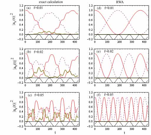
Figure 2: (Color online) Time developments of $|a_{0}(t)|^{2}$ (solid curves), $|a_{1}(t)|^{2}$ (dashed curves) and $|a_{3}(t)|^{2}$ (bold solid curve) for (a) $f=0.01$, (b) $f=0.02$ and (c) $f=0.05$ in exact calculations, and those for (d) $f=0.01$, (e) $f=0.02$ and (f) $f=0.05$ in the RWA ($g=0.01$ and $\omega=\Delta_{10}$), bottom curves in (a)-(f) expressing applied fields.

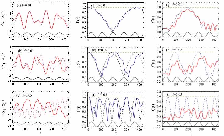
Figure 3: (Color online) (a)-(c) $\langle x_{1}+x_{2}\rangle$ for (a) $f=0.01$, (b) $f=0.02$ and (c) $f=0.05$; (d)-(f) $\Gamma(t)$ for (d) $f=0.01$, (e) $f=0.02$ and (f) $f=0.05$; (g)-(i) $C(t)$ for (g) $f=0.01$, (h) $f=0.02$ and (i) $f=0.05$, solid and dashed curves expressing results of exact and RWA calculations, respectively ($g=0.01$ and $\omega=\Delta_{10}$). Bottom curves in (a)-(i) denote applied fields.

III Model calculations

Assuming the initial ground state given by

$$a_{0}(0) = 1,\;\;a_{1}(0)=a_{2}(0)=a_{3}(0)=0,$$ (97)

we have made numerical calculations by changing model parameters of $f$, $g$ and $\omega$.

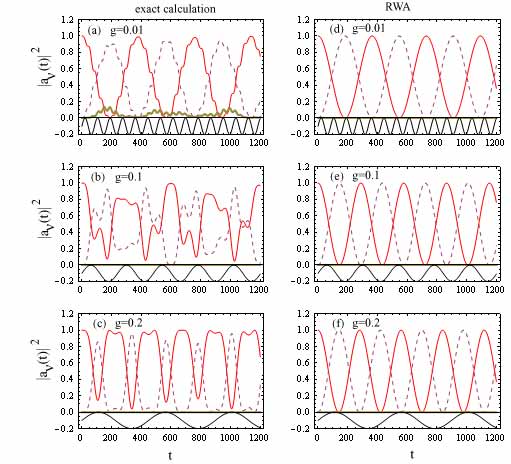
Figure 4: (Color online) Time developments of $|a_{0}(t)|^{2}$ (solid curves), $|a_{1}(t)|^{2}$ (dashed curves) and $|a_{3}(t)|^{2}$ (bold solid curve) for (a) $g=0.01$, (b) $g=0.1$, and (c) $g=0.2$ in exact calculations, and those for (d) $g=0.01$, (e) $g=0.1$, and (f) $g=0.2$ in the RWA ($f=0.01$ and $\omega=\Delta_{10}$), bottom curves in (a)-(f) expressing applied fields.

III.1 $f$ dependence

Figures 2(a), (b) and (c) show time developments of populations of $|a_{\nu}(t)|^{2}$ in levels $\nu$ ($=0,1,3$) for $f=0.0$, 0.01 and 0.02, respectively with $g=0.01$ and $\omega=\Delta_{10}$ (=0.07431) obtained by numerically solving Eqs. (54)-(57) which is hereafter referred to as an exact calculation: note that $a_{2}(t)=0$ because of $d\>a_{2}(t)/dt=0$ and $a_{2}(0)=0$. For comparison, relevant results obtained in the RWA are plotted in Figs. 2(d)-(f). Exact calculations in Fig. 2(a) show that for a field with $f=0.01$, magnitude of $|a_{0}(t)|^{2}$ is decreased while that of $|a_{1}(t)|^{2}$ is increased at $t\simeq 0$ with small $|a_{3}(t)|^{2}$, which is similar to results in the RWA shown in Fig. 2(d). For $f=0.02$, however, magnitude of $|a_{3}(t)|^{2}$ in exact calculations becomes appreciable [Fig. 2(b)] whereas it is vanishing in the RWA [Fig. 2(e)]. A comparison between Figs. 2(c) and (f) show that the difference between an exact calculation and the RWA is evident for $f=0.05$.

Figures 3(a), (b) and (c) express time dependences of $\langle x_{1}+x_{2}\rangle$ for $f=0.01$, 0.02 and 0.05, respectively, obtained by exact calculations (solid curves) and the RWA (dashed curves). We note that $\langle x_{1}+x_{2}\rangle$ shows a complicated time dependence which arises from a superposition of multiple motions with frequencies of $\omega$ and $\omega\pm\Omega$ as the RWA analysis shows. This analysis may be applied to case of $f=0.01$ and $f=0.02$. For a larger $f=0.05$, however, $\langle x_{1}+x_{2}\rangle$ of the RWA is very different from that of an exact calculation [Fig. 3(c)].

Figures 3(d), (e) and (f) show the correlation $\Gamma(t)$ calculated for $f=0.01$, 0.02 and 0.05, respectively, with $g=0.01$. RWA analysis shows that $\Gamma(t)^{2}$ oscillates with frequencies of $\omega$, $\Omega$ and $\omega\pm\Omega$.

The concurrence $C(t)$ calculated for $f=0.01$, 0.02 and 0.05 are shown Figs. 3(g), (h) and (i), respectively. At $t=0$, $C(0)=0.1485$. $C(t)$ shows complicated time dependence because $C(t)^{2}$ includes superposed oscillations with frequencies of $\omega$, $2\omega$, $\Omega$, $2\Omega$, $\omega\pm\Omega$, $2\omega\pm\Omega$ and $2(\omega\pm\Omega)$, as analyzed by the RWA which is expected to be valid for a small $f$.

III.2 $g$ dependence

Next we report calculated results when the coupling $g$ is varied. Figure 4(a), (b) and (c) show time developments of $|a_{\nu}|^{2}$ for $g=0.01$, $0.1$ and $0.2$, respectively, obtained by exact calculations with $f=0.01$ and $\omega=\Delta_{10}$ (=0.07431, 0.02611 and 0.0140 for $g=0.01$, 0.1 and 0.2, respectively). For comparison, relevant results obtained in the RWA are plotted in Figs. 4(d)-(f). A result of the RWA for $g=0.01$ in Fig. 4(d) is in fairly good agreement with that of an exact calculation in Fig. 4(a). For $g=0.1$, however, an agreement between exact and RWA calculations is not satisfactory [Fig. 4(b)]. For $g=0.2$ result of the RWA is quite different from that of an exact calculation [Fig. 4(c)].

The difference between results of $|a_{\nu}|^{2}$ in an exact calculation and the RWA reflects on expectation values of $\langle x_{1}+x_{2}\rangle$ shown in Figs.5(a)-(f). We note that although expectation values in an exact calculation and the RWA are in fairly good agreement for $g=0.01$, both the results are rather different for $g=0.1$ and 0.2.

Figs. 5(d)-(f) and Figs. 5(g)-(i) show the correlation and concurrence, respectively, obtained by an exact calculation and the RWA for several $g$ values with $f=0.01$. We note in Figs. 5(g)-(i) that the concurrence becomes larger for larger $g$. In fact, the time-averaged $\langle C_{RWA}(t)^{2}\rangle_{av}$ given by Eq. (96) is 0.383265, 0.634747 and 0.712556 for $f=0.01$, 0.02 and 0.05, respectively.

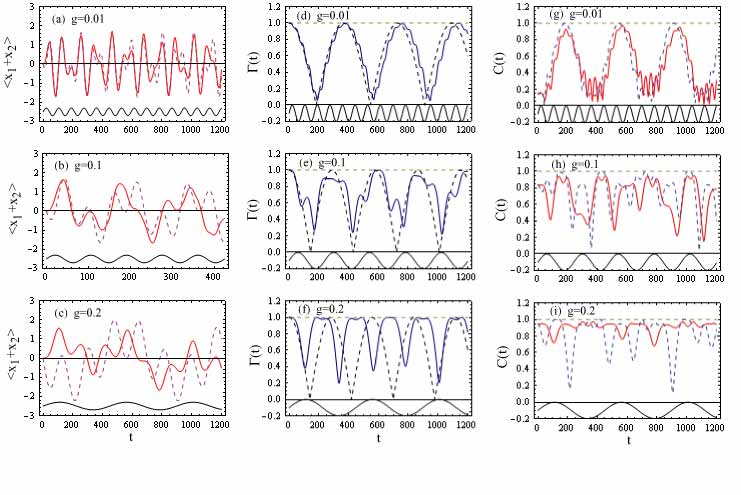
Figure 5: (Color online) (a)-(c) $\langle x_{1}+x_{2}\rangle$ for (a) $g=0.01$, (b) $g=0.1$ and (c) $g=0.2$; (d)-(f) $\Gamma(t)$ for (d) $g=0.01$, (e) $g=0.1$, and (f) $g=0.2$; (g)-(i) $C(t)$ for (g) $g=0.01$, (h) $g=0.1$, and (i) $g=0.2$, solid and dashed curves expressing results of exact and RWA calculations, respectively ($f=0.01$ and $\omega=\Delta_{10}$). Bottom curves in (a)-(i) denote applied fields.

III.3 $\omega$ dependence

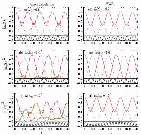
Figure 6: (Color online) Time developments of $|a_{0}(t)|^{2}$ (solid curves), $|a_{1}(t)|^{2}$ (dashed curves) and $|a_{3}(t)|^{2}$ (bold solid curve) for (a) $\omega/\Delta_{10}=0.8$, (b) $1.0$, and (c) $1.2$ in exact calculations, and those for (d) $\omega/\Delta_{10}=0.8$, (e) $1.0$, and (f) $1.2$ in the RWA ($f=g=0.01$), bottom curves in (a)-(f) expressing applied fields.

Although we have so far assumed that $\omega$ is equal to $\Delta_{10}$, its value is changed in this subsection. Figures 6(a), (b) and (c) show exact calculations of time-dependent level populations $|a_{\nu}(t)|^{2}$ for $\omega/\Delta_{10}=0.8$, 1.0 and 1.2, respectively, with $f=g=0.01$. For comparison, relevant results in the RWA are plotted in Figs. 6(d)-(f). In the resonant condition with $\omega=\Delta_{10}$, $|a_{0}(t)|^{2}$ and $|a_{1}(t)|^{2}$ oscillate between 0 and 1. It is not the case in the off-resonant condition with $\omega\neq\Delta_{10}$. We note in Figs. 10(d) and (f) that a result for $\omega/\Delta_{10}=0.8$ is the same as that for $\omega/\Delta_{10}=1.2$ in the RWA. This is because $\Omega$ is expressed in term of $(\omega-\Delta_{10})^{2}$ in Eq. (67). In exact calculations, however, a result for $\omega/\Delta_{10}=0.8$ is different from that for $\omega/\Delta_{10}=1.2$ as shown in Figs. 6(a) and (c). In particular, an exact calculation for $\omega/\Delta_{10}=1.2$ in Fig. 6(c) shows a peculiar time dependence, which is quite different from a result of the RWA in Fig. 6(f).

Time dependences of $\langle x_{1}+x_{2}\rangle$ for $\omega/\Delta_{10}=0.8$, 1.0 and 1.2 are shown in Fig. 7(a), (b) and (c) obtained by exact calculations (solid curves) and the RWA (dashed curves).

Figures 7(d)-(f) and Figs. 7(g)-(i) show the correlation function and concurrence, respectively, for $\omega/\Delta_{10}=0.8$, 1.0 and 1.2 calculated by exact calculations (solid curves) and the RWA (dashed curves). Again results of $\Gamma(t)$ and $C(t)$ in the RWA for $\omega/\Delta_{10}=0.8$ are the same as those for $\omega/\Delta_{10}=1.2$. Results of the RWA are not in good agreement with those of exact calculations except for the resonant condition of $\omega=\Delta_{10}$ with a small $f$ and a weak $g$.

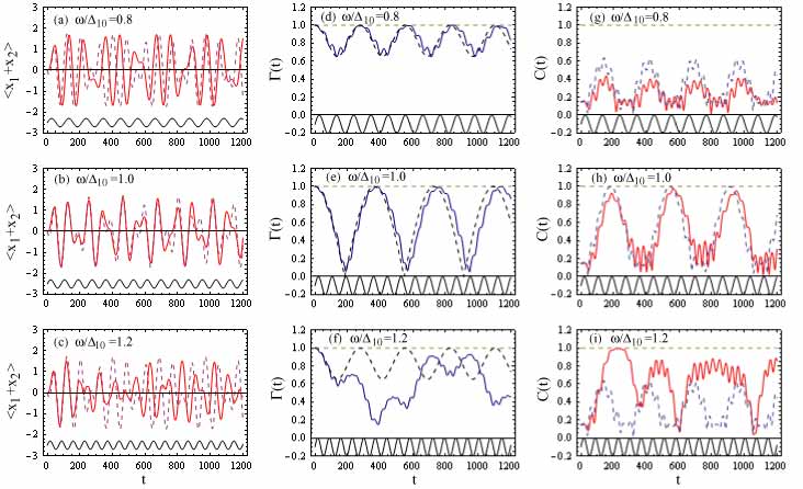
Figure 7: (Color online) (a)-(c) $\langle x_{1}+x_{2}\rangle$ for (a) $\omega/\Delta_{10}=0.8$, (b) $1.0$, and (c) $1.2$; (d)-(f) $\Gamma(t)$ for (a) $\omega/\Delta_{10}=0.8$, (b) $1.0$, and (c) $1.2$; (g)-(i) $C(t)$ for (a) $\omega/\Delta_{10}=0.8$, (b) $1.0$, and (c) $1.2$, solid and dashed curves expressing results of exact and RWA calculations, respectively ($f=0.01$ and $g=0.01$). Bottom curves in (a)-(i) denote applied fields.

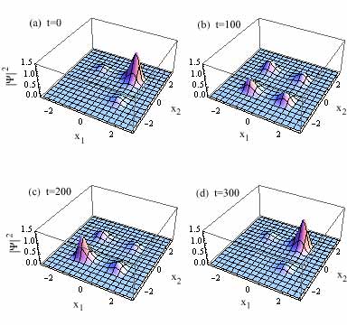
Figure 8: (Color online) Magnitudes of wavefunctions $|\Psi(x_{1},x_{2},t)|^{2}$ at (a) $t=0.0$, (b) $t=100.0$, (c) $t=200.0$ and (d) $t=300.0$ with $f=0.02$, $g=0.01$ and $\omega=\Delta_{10}$ for the initial wavepacket given by Eq. (98)

IV Discussion

IV.1 Initial wavepacket state

It would be interesting to study effects of fields applied to the initial wavepacket state given by

$$a_{0}(0) = a_{1}(0)=\frac{1}{\sqrt{2}},\;\;a_{2}(0)=a_{3}(0)=0.$$ (98)

Figure 8(a) shows the 3D plot of magnitude of $|\Psi(x_{1},x_{2},t)|^{2}$ at $t=0.0$ as functions of $x_{1}$ and $x_{2}$ with $f=0.02$, $g=0.01$ and $\omega=\Delta_{10}$, which initially has a main peak at $(x_{1},x_{2})=(1.23,1.23)$. Figures 8(b)-(d) will be explained shortly.

Figures 9(a), (b) and (c) show time developments of populations of $|a_{\nu}(t)|^{2}$ in levels $\nu$ ($=0,1,3$) for $f=0.0$, 0.01 and 0.02, respectively with $g=0.01$ and $\omega=\Delta_{10}$ ($=0.07431$) obtained by exact calculations. Relevant results obtained in the RWA are plotted in Figs. 9(d)-(f). For $f=0.0$, the populations are time independent, $|a_{0}(t)|^{2}=|a_{1}(t)|^{2}=1/2$ and $|a_{2}(t)|^{2}=|a_{3}(t)|^{2}=0.0$. For $f=0.01$, $|a_{0}(t)|^{2}$ is initially increased while $|a_{0}(t)|^{2}$ is decreased from their initial values of $1/2$ by an applied field. A result of the RWA for $f=0.01$ in Fig. 9(e) is in fairly good agreement with that of an exact calculation in Fig. 9(b). However, Figs. 9(c) and (f) show that for $f=0.02$ both results are different, in particular, a population of $|a_{3}(t)|^{2}$ becomes appreciable in an exact calculation while it is vanishing in the RWA.

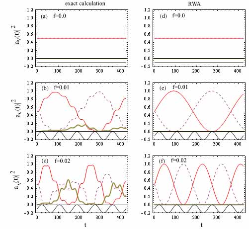
Figure 9: (Color online) Time developments of $|a_{0}(t)|^{2}$ (solid curves), $|a_{1}(t)|^{2}$ (dashed curves) and $|a_{3}(t)|^{2}$ (bold solid curve) for (a) $f=0.0$, (b) $f=0.01$ and (c) $f=0.02$ in exact calculations, and those for (d) $f=0.0$, (e) $f=0.01$ and (f) $f=0.02$ in the RWA; the initial wavepacket given by Eq. (98) is adopted with $g=0.01$ and $\omega=\Delta_{10}$. Bottom curves in (a)-(f) express applied fields.

3D plots of magnitudes of wavefunctions $|\Psi(x_{1},x_{2},t)|^{2}$ at $t=100.0$, 200.0 and 300.0 are presented in Figs. 8(b), (c) and (d), respectively. At $t=100.0$, the wavepacket has four small peaks at $(x_{1},x_{2})=(\pm 1.23,\pm 1.23)$ and $(x_{1},x_{2})=(\pm 1.23,\mp 1.23)$ [Fig.8(b)]. At $t=200.0$, it has again four small peaks at the same positions as at $t=100.0$ [Fig.8(c)] although a peak at $(x_{1},x_{2})=(-1.23,-1.23)$ is the highest among the four. The wavepacket returns approximately to the initial state at $t=300.0$ as shown in Fig. 8(d), which is similar to Fig. 8(a) at $t=0.0$.

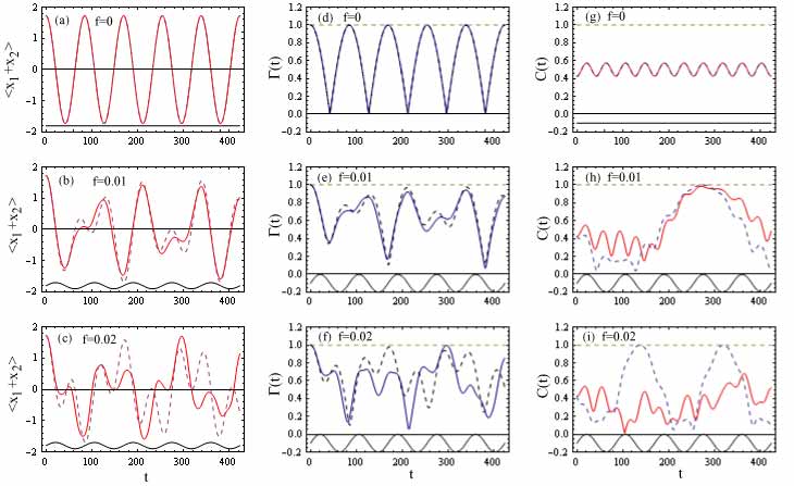
Figure 10: (Color online) (a)-(c) $\langle x_{1}+x_{2}\rangle$ for (a) $f=0.0$, (b) $f=0.01$ and (c) $f=0.02$; (d)-(f) $\Gamma(t)$ for (d) $f=0.0$, (e) $f=0.01$ and (f) $f=0.02$; (g)-(i) $C(t)$ for (g) $f=0.0$, (h) $f=0.01$ and (i) $f=0.02$, solid and dashed curves expressing results of exact and RWA calculations, respectively, for the initial wavepacket given by Eq. (98) ($g=0.01$ and $\omega=\Delta_{10}$). Bottom curves in (a)-(i) denote applied fields.

Figures 10(a), (b) and (c) express time dependences of $\langle x_{1}+x_{2}\rangle$ for $f=0.0$, 0.01 and 0.02, respectively, obtained by exact calculations (solid curves) and the RWA (dashed curves). We note in Fig. 10(a) that $\langle x_{1}+x_{2}\rangle$ for $f=0.0$ shows the simple sinusoidal time dependence, which express a tunneling of wavepacket between two minima of DW potential. When a field with $f=0.01$ is applied, both results of $\langle x_{1}+x_{2}\rangle$ obtained by exact calculations and the RWA show complicated time dependences [Fig. 10(b)]. Although the both results are in good agreement for $f=0.0$ and 0.01, results of exact and the RWA calculations become different for a larger $f=0.02$ as shown in Figs. 10(c). We note that a tunneling becomes difficult by applied fields, which is nothing but a suppression of tunneling by coherent fields Grossmann91 .

Figures 10(d), (e) and (f) show the time dependence of correlation $\Gamma(t)$ for $f=0.0$, 0.01 and 0.02, respectively, with $g=0.01$ obtained by an exact calculation (solid curves) and the RWA (dashed curves). $\Gamma(t)$ for the adopted wavepacket with $f=0.0$ is given by Hasegawa15

$$\Gamma(t)^{2} = \frac{1}{2}[1+\cos(\Delta_{10}t)],$$ (99)

which leads to a sinusoidal oscillation with a period of $2\pi/\Delta_{10}=84.55$. Figure 10(e) shows that $\Gamma(t)$ for $f=0.01$ shows complicated time dependences and that a result of the RWA is in fairly good agreement with that of an exact calculation. For a larger $f=0.02$, however, a result of the RWA becomes different from that of the exact calculation [Fig. 10(f)].

Figures 10(g), (h) and (i) show the concurrence $C(t)$ for $f=0.0$, 0.01 and 0.02, respectively, with $g=0.01$ obtained by an exact calculation (solid curves) and the RWA (dashed curves). $C(t)$ of the adopted wave packet for $f=0.0$ is given by Hasegawa15

$$C(t)^{2} = \frac{1}{4}[1+\sin^{2}(2\theta)-2\sin(2\theta)\cos(2\Delta_{10}t)],$$ (100)

which yields $C(0)=0.42577$ at $t=0.0$ for $g=0.01$. $C(t)$ for $f=0.0$ oscillates with the period of $\pi/\Delta_{10}=42.28$ as shown in Fig. 10(g). Figures 10(h) and (i) show that for finite $f=0.01$ and 0.02, $C(t)$ has complicated time dependence, just as $\Gamma(t)$.

IV.2 Step field

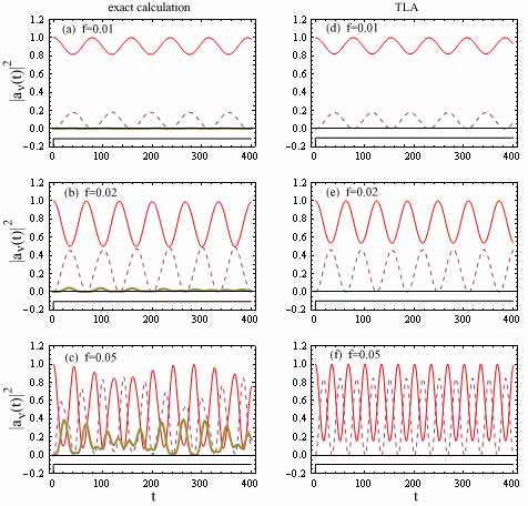
Figure 11: (Color online) Time developments of $|a_{0}(t)|^{2}$ (solid curves), $|a_{1}(t)|^{2}$ (dashed curves) and $|a_{3}(t)|^{2}$ (bold solid curve) for the applied step field with (a) $f=0.01$, (b) $f=0.02$ and (c) $f=0.05$ in exact calculations, and those for (d) $f=0.01$, (e) $f=0.02$ and (f) $f=0.05$ in the TLA ($g=0.01$), bottom curves in (a)-(f) expressing applied step fields.

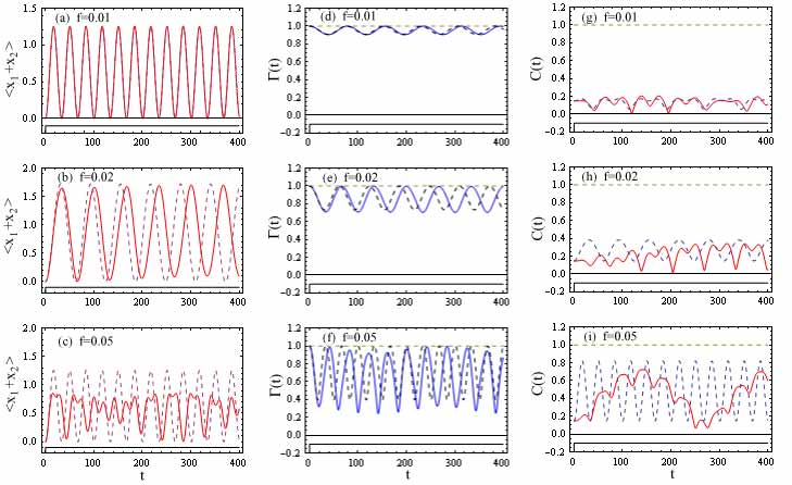
Figure 12: (Color online) (a)-(c) $\langle x_{1}+x_{2}\rangle$ for (a) $f=0.01$, (b) $f=0.02$ and (c) $f=0.05$; (d)-(f) $\Gamma(t)$ for (d) $f=0.01$, (e) $f=0.02$ and (f) $f=0.05$; (g)-(i) $C(t)$ for (g) $f=0.01$, (h) $f=0.02$ and (i) $f=0.05$, solid and dashed curves expressing results of exact and TLA calculations, respectively, ($g=0.01$). Bottom curves in (a)-(i) denote applied step fields.

Although sinusoidal periodic fields have been so far adopted, we may apply our method to any time-dependent field. As a typical example, we employ a step field given by

$$F(t) = f\>\Theta(t),$$ (101)

where $\Theta(t)$ denotes the Heaviside function.

We first try to obtain approximate analytical expressions of $a_{\nu}(t)$ ($\nu=0-3$) for an applied step field with the use of the two-level approximation (TLA) where contributions only from two terms of $a_{0}(t)$ and $a_{1}(t)$ are included. Equations (49)-(52) for $t>0$ become

$$i\hbar\>\frac{da_{0}}{dt} = -\alpha f\>e^{-i\Delta_{10}t}a_{1},$$ (102)

$$i\hbar\>\frac{da_{1}}{dt} = -\alpha f\>e^{i\Delta_{10}t}a_{0}.$$ (103)

$$i\hbar\>\frac{da_{2}}{dt} = i\hbar\>\frac{da_{3}}{dt}=0.$$ (104)

Solutions of Eqs. (102)-(104) are given by

$$a_{0}(t) = \left(\frac{\hbar}{2\alpha f}\right)[(\Delta_{10}-\Omega_{s})A\>e^{-i(\Delta_{10}+\Omega_{s})t/2}+(\Delta_{10}+\Omega_{s})B\>e^{-i(\Delta_{10}-\Omega_{s})t/2}],$$ (105)

$$a_{1}(t) = A\>e^{i(\Delta_{10}-\Omega_{s})t/2}+B\>e^{i(\Delta_{10}+\Omega_{s})t/2},$$ (106)

$$a_{2}(t) = a_{2}(0),$$ (107)

$$a_{3}(t) = a_{3}(0),$$ (108)

with

$$\Omega_{s} = \sqrt{\Delta_{10}^{2}+4(\alpha f/\hbar)^{2}},$$ (109)

where $A$ and $B$ stand for integration constants. For assumed initial conditions $a_{0}(0)=1$ and $a_{1}(0)=a_{2}(0)=a_{3}(0)=0$ which yield $A=-B=-\alpha f/\hbar\Omega_{s}$, solutions are given by

$$a_{0}(t) = \left(\frac{1}{2\Omega_{s}}\right)[(\Delta_{10}+\Omega_{s})\>e^{-i(\Delta_{10}-\Omega_{s})t/2}-(\Delta_{10}-\Omega_{s})\>e^{-i(\Delta_{10}+\Omega_{s})t/2}],$$ (110)

$$a_{1}(t) = -\left(\frac{\alpha f}{\hbar\Omega_{s}}\right)[e^{i(\Delta_{10}-\Omega_{s})t/2}-e^{i(\Delta_{10}+\Omega_{s})t)/2}],$$ (111)

$$a_{2}(t) = a_{3}(t)=0.$$ (112)

Then $|a_{0}(t)|^{2}$ and $|a_{1}(t)|^{2}$ are expressed by superposed oscillations with frequencies of $\Omega_{s}\pm\Delta_{10}$.

Figures 11(a), (b) and (c) show $|a_{\nu}|^{2}$ of exact calculations for step fields with $f=0.01$, 0.02 and 0.05, respectively, which are applied to the initial ground state given by Eq. (97); relevant results in the TLA are plotted in Figs. 11(d), (e) and (f). When a step field is applied, $|a_{\nu}(t)|^{2}$ begin to oscillate. Equations (110) and (111) may explain time dependences of $|a_{0}(t)|^{2}$ and $|a_{0}(t)|^{2}$ for small $f=0.01$ and 0.02. They are, however, not valid for $f=0.05$, for which $|a_{3}(t)|^{2}$ has an appreciable magnitude while it is assumed to be zero in the TLA.

Time dependences of $\langle x_{1}+x_{2}\rangle$, $\Gamma(t)$ and $C(t)$ are plotted in Figs. 12(a)-(c), Figs. 12(d)-(f) and Figs. 12(g)-(i), respectively, where solid and dashed curves denote results in exact calculations and in the TLA, respectively. Their time dependences for $f=0.01$ and 0.02 may be approximately elucidated in the TLA given by Eqs. (110) and (111), although they are not applicable to the case of $f=0.05$.

V Conclusion

We have studied effects of applied fields in quantum coupled DW system with the use of an exactly solvable Razavy’s potential Razavy80 . From the Schrödinger equation for the driven DW system, we have obtained equations of motion for populations of the four levels. Model calculations of expectation values $\langle x_{1}+x_{2}\rangle$, correlation $\Gamma(t)$ and concurrence $C(t)$ for applied sinusoidal fields show very complicated time dependence. Their time dependence may be analytically understood within the RWA in cases of a weak coupling and a small field in the near-resonance of $|\omega-\Delta_{10}|\ll\omega$. Otherwise, results of the RWA are not in good agreement with exact numerical calculations. It is indispensable to develop an analytical method going beyond the RWA for the DW system, just as for the TL model Ashhab07 ; Werlang08 ; Son09 ; He12 . In the present study, we do not take into account environmental effects which are expected to play important roles in real DW systems. These are left as our future subjects.

*

Appendix A A. General driving fields

We consider the input term which is more general than Eq. (4), as given by

$$H_{I} = -x_{1}F_{1}(t)-x_{2}F_{2}(t),$$ (A1)

$F_{n}(t)$ ($n=1,2$) expressing a time-dependent field applied to the $n$th DW system. The energy matrix of the time-dependent total Hamiltonian $H$ ($=H_{0}+H_{C}+H_{I}$) with basis states of $\Phi_{0}$, $\Phi_{1}$, $\Phi_{2}$ and $\Phi_{3}$ is given by

$${\cal H} = \left({\begin{array}[]{*{20}c}{E_{0}}&{-\frac{\alpha}{2}[F_{1}(t)+F_{2}(t)]}&{-\frac{\beta}{2}[F_{1}(t)-F_{2}(t)]}&{0}\\ {-\frac{\alpha}{2}[F_{1}(t)+F_{2}(t)]}&{E_{1}}&{0}&{-\frac{\beta}{2}[F_{1}(t)+F_{2}(t)]}\\ {-\frac{\beta}{2}[F_{1}(t)-F_{2}(t)]}&{0}&{\;\;E_{2}}&{\frac{\alpha}{2}[F_{1}(t)-F_{2}(t)]}\\ {0}&{-\frac{\beta}{2}[F_{1}(t)+F_{2}(t)]}&{\frac{\alpha}{2}[F_{1}(t)-F_{2}(t)]}&{E_{3}}\\ \end{array}}\right),$$ (A6)

where $\alpha$ and $\beta$ are given by Eqs. (42) and (43), respectively. Note that in the case of $F_{1}(t)=F_{2}(t)=F(t)$, Eq. (LABEL:eq:X2) becomes Eq. (LABEL:eq:A12).

With the use of Eqs. (47) and (LABEL:eq:X2), equations of motion for $a_{\mu}(t)$ ($\mu=0-3$) become

$$i\hbar\>\frac{da_{0}}{dt} = -\frac{\alpha}{2}[F_{1}(t)+F_{2}(t)]\>e^{-i\Delta_{10}t}a_{1}-\frac{\beta}{2}[F_{1}(t)-F_{2}(t)]\>e^{-i\Delta_{20}t}a_{2},$$ (A8)

$$i\hbar\>\frac{da_{1}}{dt} = -\frac{\alpha}{2}[F_{1}(t)+F_{2}(t)]\>e^{i\Delta_{10}t}a_{0}-\frac{\beta}{2}[F_{1}(t)+F_{2}(t)]\>e^{-i\Delta_{31}t}a_{3},$$ (A9)

$$i\hbar\>\frac{da_{2}}{dt} = -\frac{\beta}{2}[F_{1}(t)-F_{2}(t)]\>e^{i\Delta_{20}t}a_{0}+\frac{\alpha}{2}[F_{1}(t)-F_{2}(t)]\>e^{-i\Delta_{32}t}a_{3},$$ (A10)

$$i\hbar\>\frac{da_{3}}{dt} = -\frac{\beta}{2}[F_{1}(t)+F_{2}(t)]\>e^{i\Delta_{31}t}a_{1}+\frac{\alpha}{2}[F_{1}(t)-F_{2}(t)]\>e^{i\Delta_{32}t}a_{2}.$$ (A11)

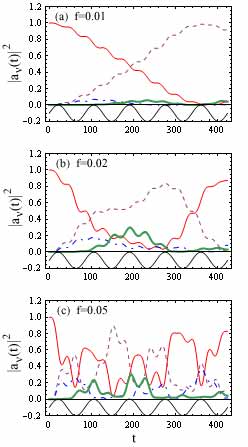
Figure 13: (Color online) Time developments of $|a_{0}(t)|^{2}$ (solid curves), $|a_{1}(t)|^{2}$ (dashed curves), $|a_{2}(t)|^{2}$ (chain curves) and $|a_{3}(t)|^{2}$ (bold solid curve) with (a) $f=0.01$, (b) $f=0.02$ and (c) $f=0.05$ in exact calculations, bottom curves in (a)-(c) expressing applied fields of $F_{1}(t)$ [$F_{2}(t)=0$].

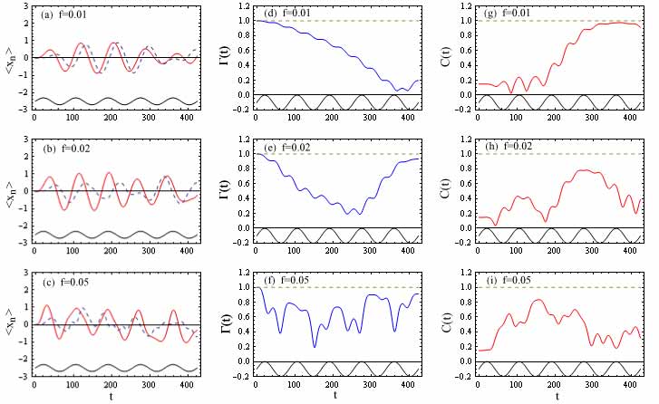
Figure 14: (Color online) (a)-(c): Time dependences of $\langle x_{1}\rangle$ (solid curves) and $\langle x_{2}\rangle$ (dashed curves) for (a) $f=0.01$, (b) $0.02$ and (c) $0.05$; (d)-(f): $\Gamma(t)$ for (d) $f=0.01$, (e) $0.02$ and (f) $0.05$; (g)-(i): $C(t)$ for (g) $f=0.01$, (h) $0.02$ and (i) $0.05$ ($g=0.01$). Bottom curves in (a)-(i) denote applied fields of $F_{1}(t)$ [$F_{2}(t)=0$].

In the symmetric case of $F_{1}(t)=F_{2}(t)=F(t)$, Eqs. (A8)-(A11) reduce to Eqs. (49)-(52). In the anti-symmetric case of $F_{1}(t)=-F_{2}(t)=F(t)$, Eqs. (A8)-(A11) become

$$i\hbar\>\frac{da_{0}}{dt} = -\beta F(t)\>e^{-i\Delta_{20}t}a_{2},$$ (A12)

$$i\hbar\>\frac{da_{1}}{dt} = 0,$$ (A13)

$$i\hbar\>\frac{da_{2}}{dt} = -\beta F(t)\>e^{i\Delta_{20}t}a_{0}+\alpha F(t)e^{-i\Delta_{32}t}a_{3},$$ (A14)

$$i\hbar\>\frac{da_{3}}{dt} = \alpha F(t)\>e^{i\Delta_{32}t}a_{2}.$$ (A15)

for which we obtain $a_{1}(t)=a_{1}(0)$.

When fields are applied only to the first DW system with $F_{1}(t)\neq 0$ and $F_{2}(t)=0$, Eqs. (A8)-(A11) yield

$$i\hbar\>\frac{da_{0}}{dt} = -\frac{\alpha F_{1}(t)}{2}\>e^{-i\Delta_{10}t}a_{1}-\frac{\beta F_{1}(t)}{2}\>e^{-i\Delta_{20}t}a_{2},$$ (A16)

$$i\hbar\>\frac{da_{1}}{dt} = -\frac{\alpha F_{1}(t)}{2}\>e^{i\Delta_{10}t}a_{0}-\frac{\beta F_{1}(t)}{2}\>e^{-i\Delta_{31}t}a_{3},$$ (A17)

$$i\hbar\>\frac{da_{2}}{dt} = -\frac{\beta F_{1}(t)}{2}\>e^{i\Delta_{20}t}a_{0}+\frac{\alpha F_{1}(t)}{2}\>e^{-i\Delta_{32}t}a_{3},$$ (A18)

$$i\hbar\>\frac{da_{3}}{dt} = -\frac{\beta F_{1}(t)}{2}\>e^{i\Delta_{31}t}a_{1}+\frac{\alpha F_{1}(t)}{2}\>e^{i\Delta_{32}t}a_{2}.$$ (A19)

For applied fields of $F_{1}(t)=f\>\sin\omega t$ and $F_{2}(t)=0$ with small $f$ and weak $g$ where $a_{2}(t)$ and $a_{3}(t)$ are negligible as will be shown shortly, we may take into account only $a_{0}(t)$ and $a_{1}(t)$. Then Eqs. (A16)-(A19) within the RWA become

$$\frac{da_{0}}{dt} = \left(\frac{\alpha f}{4\hbar}\right)\>e^{i(\omega-\Delta_{10})t}\>a_{1},$$ (A20)

$$\frac{da_{1}}{dt} = -\left(\frac{\alpha f}{4\hbar}\right)\>e^{-i(\omega-\Delta_{10})t}\>a_{0},$$ (A21)

$$\frac{da_{2}}{dt} = \frac{da_{3}}{dt}=0,$$ (A22)

which are equivalent to Eqs. (58)-(60) for the symmetric driving fields if we read $f/2\rightarrow f$.

Figures 13(a)-(c) show time developments of $|a_{\nu}(t)|^{2}$ ($\nu=0-3$) calculated for $f=0.01$, 0.02 and 0.05, respectively, with $g=0.01$ and $\omega=\Delta_{10}$ when fields of $F_{1}(t)=f\sin\omega t$ and $F_{2}(t)=0$ are applied to the system with an initial stable state given by Eq. (97). When a field with $f=0.01$ is applied, $|a_{0}(t)|^{2}$ is decreased from unity while $|a_{1}(t)|^{2}$ begins to increase at $t\sim 0.0$ with vanishingly small $|a_{2}(t)|^{2}$ and $|a_{3}(t)|^{2}$. For larger fields with $f=0.02$ and 0.05, however, magnitudes of $|a_{2}(t)|^{2}$ and $|a_{3}(t)|^{2}$ become appreciable. Results in Fig. 13(b) with $f=0.02$ are not dissimilar to those in Fig. 2(a) for the symmetrical field with $f=0.01$, as mentioned above.

Time dependences of $\langle x_{1}\rangle$ (solid curves) and $\langle x_{2}\rangle$ (dashed curves) for $f=0.01$, 0.02 and 0.05 are plotted in Figs. 14(a), (b) and (c), respectively, where $\langle x_{1}\rangle$ is different from $\langle x_{2}\rangle$: the latter seems a little delayed than the former. Note that $\langle x_{2}\rangle=0.0$ for $g=0.0$ for which the two DW systems are decoupled (related results not shown).

Relevant results of $\Gamma(t)$ for $f=0.01$, 0.02 and 0.05 are shown in Figs. 14(d), (e) and (f), respectively, while $C(t)$ are plotted in Figs. 14(g), (h) and (i). They show very complicated time dependence. It is impossible to theoretically elucidate time dependences of $|a_{\nu}(t)|^{2}$, $\langle x_{n}\rangle$ ($n=1,2$), $\Gamma(t)$ and $C(t)$ except for cases with very small $f$ and weak $g$.

References

- (1) D. J. Tannor, Introduction to quantum mechanics: A time-dependent perspective (Univ. Sci. Books, Sausalito, California, 2007).
- (2) M. Grifoni and P. Hänggi, Phys. Reports 304 (1998) 229.
- (3) F. Grossmann, T. Dittrich, P. Jung, and P. Hänggi, Phys. Rev. Lett. 67 (1991) 516.
- (4) M. J. Storcz and F. K. Wilhelm, Phys. Rev. A 67 (2003) 042319.
- (5) A. M. Satanin, M. V. Denisenko, S. Ashhab, and F. Nori, arXiv: 1201.1901.
- (6) M. Bina, S. M. Felis, arXiv: 1410.6380.
- (7) A. Pal, E. I. Rashba, and B. I. Halperin, Phys. Rev. X 4 (2014) 011012.
- (8) N. Gupta and B.M. Deb, Chemical Physics 327 (2006) 351.
- (9) M. Razavy, Am. J. Phys. 48 (1980) 285.
- (10) F. Finkel, A. Gonzalez-Lopez and M. A. Rodriguez, J. Phys. A 32 (1999) 6821.
- (11) B. Bagchi and A. Ganguly, arXiv:0302040.
- (12) H. Hasegawa, Physica E 66 (2015) 321.
- (13) W. K. Wootters, Quan. Inf. Comp. 1 (2001) 27.
- (14) S. Ashhab, J. R. Johansson, A. M. Zagoskin, and F. Nori, Phys. Rev. A 75 (2007) 063414.
- (15) T. Werlang, A. V. Dodonov, E. I. Duzzioni, and C. J. Villas-Bôoas, Phys. Rev. A 78 (2008) 053805.
- (16) S-K. Son, S. Han, and S-I. Chu, Phys. Rev. A 79 (2009) 032301.
- (17) S. He, Q. H. Chen, X. .Z Ren, T. Liu, and K. L. Wang, arXiv:1203.2410.