When do stars in 47 Tucanae lose their mass?

Abstract

By examining the diffusion of young white dwarfs through the core of the globular cluster 47 Tucanae, we estimate the time when the progenitor star lost the bulk of its mass to become a white dwarf. According to stellar evolution models of the white-dwarf progenitors in 47 Tucanae, we find this epoch to coincide approximately with the star ascending the asymptotic giant branch ($3.0\pm 8.1$ Myr before the tip of the AGB) and more than ninety million years after the helium flash (with ninety-percent confidence). From the diffusion of the young white dwarfs we can exclude the hypothesis that the bulk of the mass loss occurs on the red-giant branch at the four-sigma level. Furthermore, we find that the radial distribution of horizontal branch stars is consistent with that of the red-giant stars and upper-main-sequence stars and inconsistent with the loss of more than 0.2 solar masses on the red-giant branch at the six-sigma level.

1. Introduction

When and how a star like the Sun loses its mass to become a white dwarf star is a key open question of stellar evolution. Does the bulk of the mass loss occur when the star is a red giant or when the star reaches the asymptotic giant branch? For forty years, in stellar evolution models mass loss on the red-giant branch (RGB) has been commonly described with the Reimers (1975) formula, an empirical scaling relation that involves basic stellar parameters and an adjustable efficiency parameter, $\eta_{\rm RGB}$. This parameter is usually constrained from the requirement of reproducing the extended blue horizontal branches (HB) in the Hertzsprung-Russell diagrams of Galactic globular clusters (Renzini & Fusi Pecci, 1988). Typical values are $\eta_{\rm RGB}\simeq 0.35-0.45$, which implies that $\simeq 0.20-0.25\,M_{\odot}$ is the mass that should be lost on the red-giant branch by a star with initial mass $0.85-0.90\,M_{\odot}$, characteristic of the turn-offs in Galactic globular clusters. An additional mass loss event of smaller size, $\simeq 0.10-0.15\,M_{\odot}$, should take place later, during the evolution on the asymptotic giant branch (AGB). Recently McDonald & Zijlstra (2015) have also argued for values of $\eta_{\rm GB}=0.477\pm 0.070^{0.050}_{-0.062}$ for Galactic clusters and $\eta_{\rm GB}=0.452$ for 47 Tuc in particular.

On the other hand this classical paradigm has been recently challenged from various perspectives. Perhaps, one of the most intriguing findings is that the extended blue horizontal branch may be well explained by the very high helium abundance associated with the bluest main sequence of the multiple populations widely present in Galactic globular clusters (e.g., Lee et al., 2005; D’Antona & Caloi, 2008). In general, stellar models indicate that at the same age, higher helium corresponds to lower turn-off mass (Bertelli et al., 2008). Therefore, for the same mass ejected on the red-giant branch, a higher helium abundance favors the development of more extended horizontal branches.

At the same time there are hints that the mass loss rates predicted for red-giant-branch stars with the classical calibrations may be significantly overestimated. Using chromospheric model calculations of the H$\alpha$ line for a sample of red-giant-branch stars in a few globular clusters Mészáros et al. (2009) pointed out that the resulting mass loss rates are about one order of magnitude lower than obtained with the Reimers law or inferred from the infrared excess of similar stars by Origlia et al. (2007, see also () for recent results). Such discrepancy appears to be overcome according to Groenewegen (2012), who found agreement between the mass loss rates derived from fitting the spectral energy distributions of red-giant-branch stars with infrared excess, and the chromospheric estimates. More recently Groenewegen (2014) has performed the first detection of rotational CO line emission in a nearby red giant branch with a luminosity of $\simeq 1300\,L_{\odot}$ and an estimated mass-loss rate as low as a few $10^{-9}\,M_{\odot}$ yr^-1. Interestingly Miglio et al. (2012) argued from Kepler asteroseismic measurements of the stars in the very metal-rich open cluster NGC 6971 that low values of $\eta$ on the red-giant branch ($\eta_{\mathrm{RGB}}$) are needed to account for the mass loss between the red giant and red clump phases of stars in this metal-rich cluster ($0.1\lesssim\eta_{\mathrm{RGB}}\lesssim 0.3$).

On the other hand, mass loss on the asymptotic giant branch of old stellar populations may have been underestimated at lower metallicities. Recent stellar population synthesis studies have shown that to reproduce the star counts and luminosity functions of metal-poor low-mass thermally-pulsing asymptotic-giant branch (TP-AGB) stars in a sample of nearby galaxies one has to invoke a more efficient mass loss than the classical Reimers recipe (Girardi et al., 2010; Rosenfield et al., 2014, see Sect. 2). This also yields good agreement with the low-mass end of the initial-final mass relation, as probed with the white dwarfs in M 4 (Kalirai et al., 2009).

In this study we build upon the results of Heyl et al. (2015) to demonstrate that the bulk of the mass loss from stars in 47 Tucanae must happen on the asymptotic giant branch. In the core of the globular cluster 47 Tucanae the timescale for dynamical relaxation through two-body interactions is similar to the stellar evolution timescale for a star to live as a horizontal-branch star, rise up the asymptotic branch and become a white-dwarf star (Harris, 1996; Heyl et al., 2015). The core of 47 Tuc has been the focus of numerous previous investigations (e.g McLaughlin et al., 2006; Knigge et al., 2008; Bergbusch & Stetson, 2009; Milone et al., 2012a), but Heyl et al. (2015) is the first paper that combines the near ultraviolet filters of the Hubble Space Telescope (HST) with a mosaic that covers the entire core of the cluster. In these filters the young white dwarfs, the giant stars, the horizontal-branch stars, the blue stragglers and the upper main sequence stars all have similar magnitudes as shown in Fig. 2. Furthermore, the exquisite angular resolution in the near ultraviolet of the new Hubble WFC3/UVIS camera also reduces the effects of confusion and incompleteness in this crowded field. From theoretical arguments it has long been argued that two-body interactions will sort the stars in a globular cluster by mass with the more massive stars lying closer to the center of the cluster (e.g. Spitzer, 1987), and this mass segregation has been quantified in various clusters (e.g Goldsbury et al., 2013). Heyl et al. (2015) for the first time caught this process of mass segregation in action and determined the timescale for the sorting of stars by mass, the relaxation time, to be about 30 Myr. They have outlined in detail how to measure the completeness rate and model the diffusion of stars in the cluster using the young white dwarfs.

Here we build upon this diffusion model by comparing the radial distribution of the white dwarfs with that of the upper-main-sequence and red-giant stars. The key observation that one can draw from Fig. 2 is that the distribution of the bright white dwarfs, whose median age along the white-dwarf cooling track is 6 Myr, more closely resembles that of the upper-main-sequence stars than that of the fainter white dwarfs of about 100 Myr. If the progenitors of the white dwarfs lost their mass more than 30 Myr before the birth of the white dwarfs, the white dwarfs would have already been sorted by mass, so their radial distribution would not look so similar to that of the upper-main sequence stars. Furthermore, because the horizontal branch in 47 Tucanae is thought to last for about 80 Myr, a few relaxation times, their radial distribution will also reflect the mass of the horizontal branch stars. The radial distribution of the horizontal branch stars is very similar to that of the upper-main-sequence stars, their progenitors. We will confront these observations with expectations from stellar evolution models and better quantify it with the diffusion models from Heyl et al. (2015).

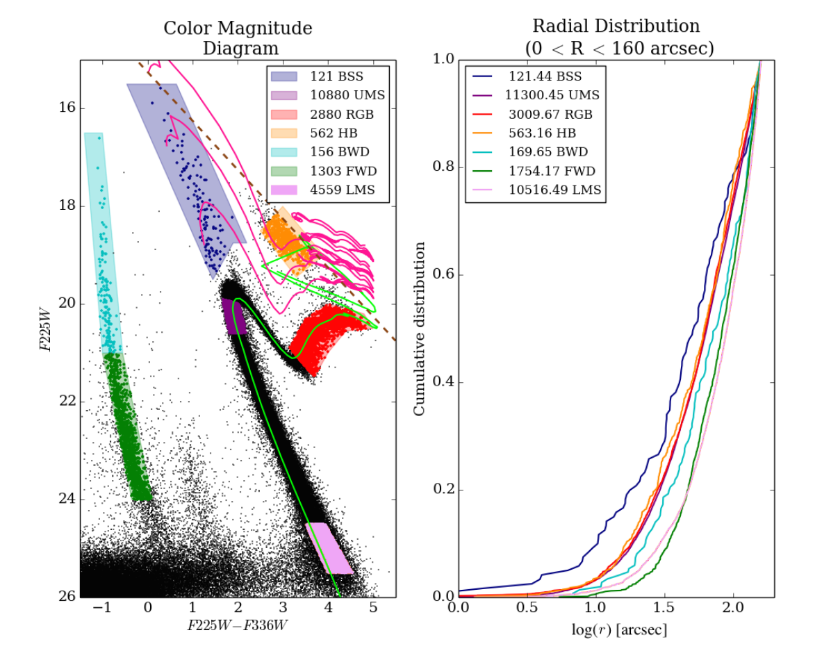
Figure 1.— Left: Color-magnitude diagram of the core of 47 Tucanae in the WFC3 filters F225W and F336W. We have imposed a mild cut on magnitude error to remove strong saturated stars from the sample. The inset gives the number of stars in each class before correcting for completeness. The classes are: BSS, blue straggler stars; UMS, upper-main-sequence stars of about $0.9\mathrm{M}_{\odot}$; RGB, red-giant-branch stars; HB, horizontal-branch stars; BWD, bright white dwarfs; FWD, faint white dwarfs; and LMS, lower-main-sequence stars of about $0.65\mathrm{M}_{\odot}$. We determine locations of these classes on the color-magnitude diagram from the PARSEC isochrones and the MESA evolutionary models. The magenta curves trace evolutionary tracks calculated with MESA and the atmosphere models of Castelli & Kurucz (2004). The magenta curves from bottom to top are for initial masses of 1.1, 1.4 and 1.8 solar masses. We have assumed that the post-main sequence of the blue-straggler stars follows a similar track to normal stars of a similar mass (Sills et al., 2009). The green curve is a PARSEC isochrone for an age of 11 Gyr and the metallacity of 47 Tucanae using the bolometric corrections of Chen et al. (2014). An additional 0.4 and 0.3 magnitudes of extinction were added in F225W and F336W respectively to fit the isochrone to the data. The dashed line traces $F336W=15.25$, the approximate magnitude where the images are saturated, so model curves to the right of this line will have observed colors just to the left of the line. Right: The completeness-corrected radial distribution of stars in the various regions highlighted in the color-magnitude diagram. The radial distribution of the upper-main sequence stars (UMS) and the red giants (RGB) are nearly indistinguishable. Here the inset gives the size of each sample after correcting for completeness.

2. Stellar Evolution Models

To construct the stellar evolution models here, we used both MESA (Modules for Experiments in Stellar Astrophysics; Paxton et al. 2011) and a combination of PARSEC (for the evolution before the TP-AGB; Bressan et al. 2012) and COLIBRI (for the TP-AGB; Marigo et al. 2013) to perform simulations of stellar evolution starting with a pre-main-sequence model of 0.9 solar masses and a metallicity of $Z=4\times 10^{-3}$ and $Y=0.256$, appropriate for the cluster 47 Tucanae (Bergbusch & Stetson, 2009), assuming $[\mathrm{Fe/H}]=-0.83$ and $[\alpha/\mathrm{Fe}]=0.3$. We note that adopting $[\mathrm{Fe/H}]=-0.76$ and individual elemental abundances measured in 47 Tuc stars (as summarized in Milone et al., 2012a) leads to a somewhat larger metallicity ($Z\sim 0.0055$), but the general trends, discussed below, do not change significantly.

For the MESA models, we used SVN revision 5456 and started with the model 1M_pre_ms_to_wd in the test suite. We changed the parameters initial_mass and initial_z of the star and adjusted the parameter log_L_lower_limit to $-6$ so the simulations run well into the white dwarf cooling regime. We also reduced the values of the wind $\eta$ on the RGB and AGB to 0.46 (from the default of 0.7) to yield a 0.53 solar mass white dwarf (Renzini & Fusi Pecci, 1988; Moehler et al., 2004; Kalirai et al., 2009) from the 0.9 solar mass progenitor. The MESA models are consistent with the observed $M_{V}$ of the tip of the TP-AGB (Lebzelter & Wood, 2005) which is sensitive to the mass of the resulting WD and with the observed cooling curve of the white dwarfs (Heyl et al., 2015). For the mass loss on the red-giant branch we used the Reimers (1975) value,

$${\dot{M}}_{R}=4\times 10^{-13}\eta\frac{L}{L_{\odot}}\frac{R}{R_{\odot}}\frac{M_{\odot}}{M}\,\,\,\,\,\,\,\,\,\,\,\,\,[{M_{\odot}}{\mathrm{yr}}^{-1}]$$ (1)

and on the asymptotic-giant branch we use the Blöcker (1995) formula

$${\dot{M}}_{B}=4.83\times 10^{-9}\left(\frac{M}{M_{\odot}}\right)^{-2.1}\left(\frac{L}{L_{\odot}}\right)^{2.7}{\dot{M}}_{R}.$$ (2)

These parameters yield a model where the star loses about 0.2 solar masses as a red giant and 0.17 solar masses as an asymptotic giant star. As other options we also used a value of $\eta$ on the red-giant branch of 0.1, 0.2 and 0.3 in the range of Miglio et al. (2012) and higher values on the AGB ($\eta_{\mathrm{AGB}}$) as outlined in Table 1. These also yielded a 0.53 solar mass white dwarf but with much less mass loss on the red-giant branch with values of $\eta$ in better accordance with the results of Miglio et al. (2012).

Table 1 summarizes the results of the various wind models using MESA. Essentially the two wind parameters $\eta_{\mathrm{RGB}}$ and $\eta_{\mathrm{AGB}}$ can be tuned to change the ratio of mass loss on the two giant branches without changing the initial or final mass of the star (here $0.9$ and $0.53\mathrm{M}_{\odot}$), the age of the star where it becomes a white dwarf at the tip of the AGB ($t_{\mathrm{WD}}$) — this should equal the age of the globular cluster today. We examine two other timescales. The first is the time interval between the tip of the red-giant branch and the tip of the asymptotic giant branch, $\Delta t_{\mathrm{T2T}}$, and the second is the time between the helium flash and when the central helium abundance drops below $10^{-5}$, $\Delta t_{\mathrm{CHB}}$, the epoch of core helium burning. During the core helium burning stage of the star, the luminosity remains nearly constant for about 80 Myr, somewhat less than these two timescales, according to the PARSEC evolutionary tracks. This is the expected time that stars will linger within the region of the CMD denoted as the horizontal branch in Fig. 2. When the two wind parameters are equal, the mass loss on the two branches also ends up being about equal and using the range of parameters outlined by Miglio et al. (2012) one can have as little as one-ninth of the mass loss on the red-giant branch, leaving nearly ninety percent of the mass loss to occur on the asymptotic giant branch.

Table 1Wind Parameters for the Various MESA Models.

$\eta_{\mathrm{RGB}}$	$\eta_{\mathrm{AGB}}$	$M_{\mathrm{HB}}$	$M_{\mathrm{WD}}$	$\Delta t_{\mathrm{T2T}}$	$\Delta t_{\mathrm{CHB}}$	$t_{\mathrm{WD}}$
		[$M_{\odot}$]	[$M_{\odot}$]	[Myr]	[Myr]	[Gyr]
0.1	0.7	0.86	0.54	108	89.2	10.8
0.2	0.6	0.82	0.54	109	89.7	10.8
0.3	0.5	0.78	0.53	110	90.4	10.8
0.46	0.46	0.70	0.53	111	91.0	10.9

The procedure for the PARSEC-COLIBRI models was similar, but for the mass-loss descriptions. A first set of models was computed adopting the Reimers law on the RGB, in combination with the Schröder & Cuntz (2005) formula for the TP-AGB, as modified by Rosenfield et al. (2014):

$$\begin{split}{\dot{M}}_{\rm mSC}=10^{-12}\eta_{\rm mSC}\frac{L}{L_{\odot}}\frac{R}{R_{\odot}}\frac{M_{\odot}}{M}\left(\frac{T_{\rm eff}}{4000\,{\rm K}}\right)^{8.9}\\ \left(1+\frac{g_{\odot}}{4300g}\right)\,\,\,\,\,\,\,\,\,\,\,\,\,[{M_{\odot}}{\mathrm{yr}}^{-1}]\end{split}$$ (3)

where $g=GM/R^{2}$ is the surface gravity, and $\eta_{\rm mSC}$ is a free efficiency parameter. Again for each value of $\eta_{\mathrm{RGB}}=0.1,0.2,0.3,0.4$, the parameter $\eta_{\rm mSC}$ of the AGB mass loss was tuned so as to obtain a final C-O core with mass of $\simeq 0.53-0.54\,M_{\odot}$. We also found that the tip of the TP-AGB in PARSEC-COLIBRI models was consistent with the observed $M_{V}$ at the tip of the TP-AGB in 47 Tuc (Lebzelter & Wood, 2005).

We recall that Eq. (3) was proposed by Rosenfield et al. (2014) with the purpose of reproducing the star counts and luminosity functions of TP-AGB stars detected in a sample of nearby metal-poor galaxies from the ACS Nearby Galaxy Survey Treasury (ANGST; Dalcanton et al., 2009), which do not present signs of recent star formation. The working scenario is that at lower luminosities on the AGB winds are not driven by dust opacity, rather they should be linked to the mechanical flux produced in highly turbulent chromospheres (Cranmer & Saar, 2011). Adopting $\eta_{\mathrm{RGB}}=0.2$ for RGB stars, the ANGST data were best reproduced assuming that on the TP-AGB low-metallicity low-mass stars experience more mass loss than predicted by the classical Reimers law (with $\eta_{\mathrm{RGB}}=0.3-0.4$). Good agreement with observations was obtained by setting the efficiency parameter $\eta_{\rm mSC}=0.4$ in the modified Schröder & Cuntz (2005) formula. The calibration also sets constraints on the TP-AGB lifetimes for $\mathrm{[Fe/H]}\lesssim-0.9$. They should be $\sim 0.5$ Myr for lower mass stars ($M\lesssim 1\,M_{\odot}$), corresponding to final masses of $0.52-0.54\,M_{\odot}$.

A second test calculation was performed with the prescriptions recently proposed by Origlia et al. (2014) to describe mass loss on both the RGB and the AGB of Galactic globular clusters. This formulation was derived relating the mid-IR excess exhibited by a fraction of RGB stars to the mass-loss rate, through a scaling relation that involves a few parameters for the dust properties. We set the parameters equal to the reference values suggested by the authors for 47 Tucanae, namely: expansion velocity $\upsilon_{\mathrm{exp}}=10$ km s^-1, gas-to-dust ratio $\delta=200$, and grain density $\rho=3$ g cm^-3. Another quantity to be specified is the fraction $f_{\rm on}$ of dusty RGB stars, which may vary with the bolometric magnitude $M_{\rm bol}$. Its value was derived from Fig. 4 of Origlia et al. (2014) paper. Assuming $\mathrm{[Fe/H]}=-0.7$ for 47 Tucanae, we got $f_{\rm on}=0.098$ for $-1.5\leq M_{\rm bol}\leq-0.6$ and $f_{\rm on}=0.222$ for $M_{\rm bol}<-1.5$ on the RGB; $f_{\rm on}=0.292$ for $M_{\rm bol}<-1.5$ on the AGB. No mass loss was considered for $M_{\rm bol}>-0.6$.

A third test calculation was carried out using another semi-empirical mass loss relation based on the measured infrared excess. With the aid of dust radiative transfer calculations that best fit the observed spectral energy distributions of a sample of field RGB stars, with accurate parallaxes, Groenewegen (2012) derived the formula

$${\dot{M}}_{R}=4\times 10^{-14}\left(\frac{L}{L_{\odot}}\frac{R}{R_{\odot}}\frac{M_{\odot}}{M}\right)^{0.90}\,\,\,\,\,\,\,\,\,\,\,\,\,[{M_{\odot}}{\mathrm{yr}}^{-1}]\,.$$ (4)

We note that there is no adjustable parameter here, and that the reference dust parameters used by Groenewegen (2012) were $\delta=200$, and $\upsilon_{\mathrm{exp}}=10$ km s^-1, which are exactly the same as the ones adopted in the Origlia et al. (2014) formulation. Instead, as we will see below, the predictions in terms of RGB mass loss are significantly different! Later on the AGB mass loss was described with the modified Schröder & Cuntz (2005) formula given by Eq. (3). An efficiency parameter $\eta_{\rm mSC}=0.8$ was found to be the suitable choice to obtain a final mass of $\simeq 0.54\,M_{\odot}$.

Table 2 outlines the results of the PARSEC-COLIBRI models. The quantitative trends are quite similar to those obtained with the MESA code. Small differences in the mass on the horizontal branch for the same $\eta_{\mathrm{RGB}}$ can be easily explained by the details of the model. Concerning the model with the Origlia et al. (2014) mass loss, we just note that it yields a final mass of $0.57\,M_{\odot}$, that is larger than our reference value of $0.53\,M_{\odot}$. In fact, with the Origlia et al. (2014) formula for mass loss the TP-AGB star is predicted to experience 9 thermal pulses before leaving the AGB, while in all other COLIBRI models the total number of thermal pulses is $\simeq 3-4$. The corresponding lifetime is therefore longer, $\simeq 2.1$ Myr, compared to $\simeq 0.5-0.9$ Myr for the set of TP-AGB calculations made with the modified Schröder & Cuntz (2005) relation.

Even though the method to derive the mass-loss rates for RGB stars is intrinsically similar to that adopted by Origlia et al. (2014), i.e. dust radiative transfer calculations that best fit the spectral infrared excess, the predictions for RGB mass loss obtained with the semi-empirical relation of Groenewegen (2012) are completely different.

Table 2Wind Parameters for the Various PARSEC/COLIBRI Models.

$\eta_{\mathrm{RGB}}$	$\eta_{\mathrm{mSC}}$	$M_{\mathrm{HB}}$	$M_{\mathrm{WD}}$	$\Delta t_{\mathrm{T2T}}$	$\Delta t_{\mathrm{CHB}}$	$t_{\mathrm{WD}}$
		[$M_{\odot}$]	[$M_{\odot}$]	[Myr]	[Myr]	[Gyr]
0.1	0.7	0.84	0.54	107	94.5	10.98
0.2	0.5	0.79	0.54	108	94.9	10.98
0.3	0.3	0.72	0.53	111	97.9	10.98
0.4	0.13	0.65	0.53	109	95.4	10.98
Or14	Or14	0.69	0.57	111	97.9	10.98
Gr12	0.8	0.88	0.54	108	96.0	10.98
References.		Or14:Origlia et al. (2014)
		Gr12:Groenewegen (2012)

3. The Epoch of Mass Loss

Through an analysis of the distribution of magnitudes and positions of the young white dwarfs in the core of 47 Tucanae, Heyl et al. (2015) measured the rate of diffusion due to relaxation in the cluster. The right panel of Fig. 2 depicts the radial distribution of the brighter and fainter white dwarfs. Both groups of white dwarfs have the nearly same mass because they formed from stars of similar mass. The mass of the turn-off in 47 Tucanae varies by about 0.3% over 100 Myr, and the mass of the resulting white dwarf would vary by 0.05% over this same period. However, the fainter ones were formed earlier, so they have been diffusing through the cluster for a longer time. We have also added the radial distribution of the stars on the upper main sequence. This distribution is only slightly more concentrated than the young white dwarfs, indicating that there has been very little time for the young white dwarfs to have diffused through the cluster since their progenitors lost mass. Furthermore, the distribution of the upper-main-sequence stars is nearly identical to that of the red-giant branch stars even when we focus on seven-hundred stars near the tip of the red-giant branch. Using the white-dwarf formation rate from Heyl et al. (2015) and the PARSEC models depicted in Fig. 2, this corresponds to the last hundred million years along the red-giant branch, indicating that little mass loss has occurred up to about 100 Myr before the tip of the RGB. In particular one can pose the question how much diffusion has occurred between the upper main-sequence or equivalently the RGB and the young white dwarfs.

We can play the diffusion back in time to what is presumably the initial radial distribution of the stars, that of stars on the upper main sequence or the giants as depicted in Fig. 2. We assume a cooling curve for the white dwarfs and the best-fitting two-Gaussian model for the distribution of the white dwarfs as they diffuse; all that we vary is the time for main-sequence radial distribution to diffuse and to appear like the distribution of white dwarfs younger than 50 Myr. We fit for the best-fitting timescales by performing a Kolmogorov-Smirnov test between the diffusion model and the distribution of stars. Fig. 2 depicts the best-fitting diffusion models along with the observed distributions.

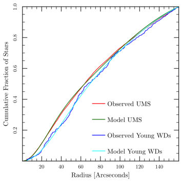
Figure 2.— Radial distribution of the upper-main sequence stars as depicted in Fig. 2 and the white dwarfs younger than 50 Myr. There are 367 young white dwarfs, and their median age is 18.9 Myr since the tip of the AGB. The diffusion time between the two model distributions is 21.9 Myr.

If we assume a cooling curve for the white dwarfs as described in § 2 and a two-Gaussian model for the diffusion, we find that the mass-loss event coincides with the tip of the AGB, and the mass loss greater than 0.2 solar masses earlier than 20 Myr before the tip of the AGB can be excluded with ninety-percent confidence. A major mass-loss event on the RGB (greater than 0.2$M_{\odot}$ can be excluded at the greater than the four-sigma level ($p<10^{-8}$) from the diffusion of the youngest white dwarfs alone.

Fig. 3 and 4 also depict the Kolmogorov-Smirnov probability obtained by evaluating the diffusion time-scale required to go from the best-fitting model for the UMS stars to the best-fitting model for a sample of young WDs (median age of 18.9 Myr since the tip of the AGB) as depicted in Fig. 2. This brings the epoch of major mass loss practically coincident with the TP-AGB. This probability assumes that the theoretical diffusion model is fixed; in particular, it does not include the approximately ten-percent uncertainty in the diffusion timescale. This would shift the peak of the probability about 2 Myr in either direction. The statistical standard deviation in determining the median age of the white-dwarf sample is 1.2 Myr. The theoretical cooling curve itself also yields an additional uncertainty in the diffusion timescale of about 4 Myr. This is obtained by comparing of the theoretical cooling curve with the empirical cooling curve (Goldsbury et al., 2012). Combining these uncertainties in quadrature yields the result that the mass-loss should have taken place $3.0\pm 8.1$ Myr before the tip of the AGB.

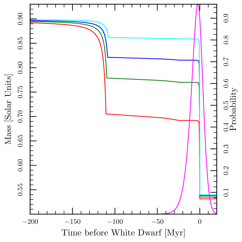
Figure 3.— Mass of a star that will become a modern-day white dwarf in 47 Tucanae as a function of time before its peak luminosity for the MESA models. The first epoch of mass loss in the model is as a red giant and the second is as an asymptotic giant star. The lowermost curve traces the mass loss for $\eta_{\mathrm{RGB}}=\eta_{\mathrm{AGB}}=0.46$ and the upper curves trace the mass loss for $\eta_{\mathrm{RGB}}=0.1,0.2$ and $0.3$ from top to bottom with the other quantities given in Table 1. The magenta curve depicts the KS probability of the epoch of mass loss obtaining calculating the diffusion of the UMS stars over a given time interval and comparing the resulting radial distribution with that of the young white dwarfs (median age 18.9 Myr) — the best fitting time for the mass loss to have occurred coincides with the TP-AGB.

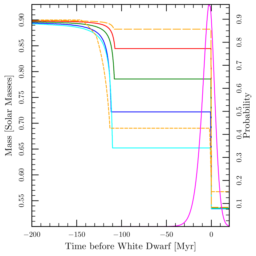
Figure 4.— Mass of a star that will become a modern-day white dwarf in 47 Tucanae as a function of time before its peak luminosity for the COLIBRI models. From top to bottom the four curves (solid lines) trace the mass loss for $\eta_{\mathrm{RGB}}=0.1,0.2,0.3$, and $0.4$ with the other quantities given in Table 2. The short-dashed line corresponds to the Origlia et al. (2014) formulations for mass loss, while the uppermost long-dashed line refers to the mass-loss rates predicted by Groenewegen (2012) for the RGB and with the modified Schröder & Cuntz (2005) relation for the AGB. Note that in both cases the RGB mass loss is derived from the results of the semi-empirical infrared-excess method, with quite different results.

The indications from the diffusion modelling show that the bulk of the mass loss is likely to have occurred while the white dwarf progenitors ascended the asymptotic giant branch. The distribution of the young white dwarfs closely resembles that of the upper main sequence stars because they have not had time to relax to their new mass. It is unclear whether all of the mass loss occurs on the asymptotic giant branch or just the bulk of it. From these dynamical arguments it is likely that the mass-loss evolution calculated from the MESA model with equal values of $\eta$ depicted by the lowermost curve in Fig. 3 is not correct. In this case during the first mass loss event, the mass of the progenitor decreases by 0.20 solar masses on the red-giant branch and 0.17 solar masses on the asymptotic giant branch. Similar considerations apply to the PARSEC-COLIBRI models as depicted in Fig. 4 with $\eta_{\mathrm{RGB}}=0.4$. In this case the mass lost on the red-giant branch, 0.25 solar masses, is even larger, by a factor of two, than the mass expelled on the asymptotic giant branch, 0.12 solar masses. The model computed with the Origlia et al. (2014) formalism predicts similar amounts of ejected masses, with the notable difference that the final mass and the TP-AGB lifetime are larger. Two of the diffusion models point to the AGB as the location of the mass loss, so it is likely that even more than two-thirds of the mass loss occurs then.

The conclusion is that in 47 Tuc the mass of the horizontal-branch should be not much different from that the main-sequence stars. Miglio et al. (2012) argued from asteroseismic observations of red giant and red clump stars in NGC 6791 that at least in this metal-rich cluster little mass is lost on the red-giant branch, less than a tenth of a solar mass. If we use the value of $\eta=0.2$ as suggested by Miglio et al. (2012) the mass of the star decreases more on the AGB as traced by the second curve from the top in Fig. 3. Here the star only loses 0.08 solar masses on the red-giant branch and 0.28 solar masses on the AGB in better accordance with the diffusion models. The predictions of mass loss with the PARSEC-COLIBRI model are of 0.11 and 0.25 solar masses, respectively for $\eta_{\mathrm{RGB}}=0.2$ and $\eta_{\mathrm{mSC}}=0.5$. Further support to the findings of our diffusion models comes from the RGB mass loss rates derived by Groenewegen (2012) from the measured infrared excess in a sample of field RGB stars. In fact, adopting his proposed formulation we obtain that only $\approx 0.02\,M_{\odot}$ is expelled on the RGB, so that the star reaches the AGB with a mass that is in practice the same it had on the main sequence. In this case $\approx 0.34\,M_{\odot}$ is lost on the AGB. We emphasize that the agreement was obtained with the original Groenewegen (2012) relation for the RGB mass loss rates, without introducing any efficiency parameter. Moreover, as discussed by Groenewegen (2012), the mass-loss rates derived in his study are consistent with the chromospheric estimates for RGB stars. It also appears that, surprisingly, the winds in metal-rich stars may operate similarly to those in more metal-poor stars such as in 47 Tuc.

The radial distribution of the horizontal-branch stars themselves may help to constrain their masses. The core-helium burning phase on the horizontal branch lasts for about 100 Myr and stars will linger in the region of CMD that we define as the horizontal branch for about 80 Myr; this is more than a relaxation time of 30 Myr (Heyl et al., 2015), so if there is a significant amount of mass loss before the horizontal branch, one would expect the horizontal-branch stars to be less concentrated than the upper main sequence. Fig. 2 shows that the horizontal branch of the evolved blue-straggler stars could contaminate the HB region of the CMD due to saturation. To remove the saturated stars from the sample we have imposed a mild cut on the uncertainty in the magnitude estimates. Fig. 2 also depicts the radial distribution of the giants and horizontal-branch stars. The giant stars have a similar distribution to the upper-main sequence, and so do the horizontal-branch stars. If the horizontal-branch stars and the upper-main sequence stars were drawn from the same distribution, one would expect to find a deviation in the cumulative distribution as large as observed more than one third of the time (using the Kolmogorov-Smirnov test). Furthermore the number of horizontal branch stars after correcting for incompleteness (563) is in loose agreement with the theoretical duration of the horizontal branch of 80 Myr and the birth rate of white dwarfs in the field of about 7 Myr^-1 (Heyl et al., 2015).

Fig. 2 also depicts the radial distribution of main-sequence stars whose mass is about $0.65\mathrm{M}_{\odot}$ as determined from the PARSEC isochrone (in lavender); the distribution nearly coincides with the faint white dwarfs (in green). If the mass of the horizontal branch were $0.65\mathrm{M}_{\odot}$, this is the radial distribution to which the HB branch stars would ultimately relax. Of course, this would take about 100 Myr to reach completion, and the average age of a horizontal branch star is only 40 Myr but the bulk of the relaxation would occur within 40 Myr. The null hypothesis that the horizontal branch and the main-sequence stars of a mass of about $0.65\mathrm{M}_{\odot}$ are drawn from the same radial distribution can be rejected by a Kolmogorov-Smirnov test at the six-sigma level ($p\approx 3\times 10^{-17}$).

By comparing the distribution of upper-main-sequence stars, giant stars, horizontal branch stars, young and old white dwarfs, we find that it is most likely that the stars that are currently evolving to form white dwarfs lose more mass as asymptotic giant branch stars than as red-giant-branch stars. In the context of the Reimers and Blöcker or modified Schröder & Cuntz models for wind mass loss, parameters such as $\eta_{\mathrm{RGB}}\approx 0.1$ and $\eta_{\mathrm{AGB}}\approx 0.7$ best account for the observed radial distributions of the stars. Conversely, all wind descriptions that predict the bulk of mass loss on the RGB conflict with the indications presented in this work.

4. Conclusions

We must emphasize that the results presented here proceed from two independent observations. The first is an inference of the time-scale of the major mass loss which rules out the RGB in favor of the AGB phase. This conclusion is nearly independent of the assumed distance to 47 Tucanae and the models of the horizontal-branch evolution. The time scale that we derive rests on three independent arguments: the dynamical relaxation time from theoretical considerations, the white-dwarf cooling timescale and the duration of the red-giant-branch evolution that can be used to estimate the ages of the white dwarfs without reliance on white-dwarf cooling models (Heyl et al., 2015) — we count the number of red-giant stars in the CMD and determine the white-dwarf birthrate from the theoretical evolutionary timescale through this portion of the CMD (see Goldsbury et al., 2012, for further details). All three agree and point to the AGB as the origin of the mass loss.

Furthermore, even a large relative error in these timescales would only result in a slight change in the timescale of the mass loss relative to the duration of the horizontal branch because we are measuring the time elapsed between the mass-loss event and the appearance of a young $\sim 20$ Myr white dwarf. We find this to be about 20 Myr, so our estimate of the diffusion timescale would have to be underestimated by a factor of five to place the bulk of the mass loss on the red-giant branch. In this case it would be difficult to account for the diffusion between the bright and faint white dwarfs unless the white-dwarf cooling timescale were also underestimated by a factor of five, and the white-dwarf birthrate were overestimated by a factor of five as well. Because the white dwarfs are produced through stellar evolution, a revision of the white-dwarf birth rate would require a revision of the timescales for the entire post-main-sequence stellar evolution to achieve consistency with the numbers of stars observed in the CMD of 47 Tuc. In particular this would also increase the duration of the horizontal branch by about a factor of five as well, leading to further theoretical and observational inconsistencies.

The second line of evidence rests on the observed radial distribution of horizontal branch stars that strongly resembles the distribution of the upper-main sequence stars. The horizontal branch lasts long enough to suffer from diffusion if a significant amount of mass loss occurs before it. By using a mild cut in magnitude error we have eliminated the most saturated stars from our horizontal-branch sample. As shown in Fig. 2, these saturated stars are most likely the descendents of the blue-straggler stars. The number of horizontal branch stars in the field is also in accord with theoretical models and rate of formation of white dwarfs in the field.

Our conclusions face two possible difficulties: the presence of multiple populations in 47 Tuc (Anderson et al., 2009; Milone et al., 2012b) and the conclusion from the current state of the art of horizontal-branch modelling that more mass loss is required to account for the observed horizontal branch (di Criscienzo et al., 2010). Milone et al. (2012b) found that the second generation dominates the population most strongly in the center of the cluster and the ratio of the two populations is constant with radius within the error bars where our observations focus. Although Richer et al. (2013) found dynamical signatures and a radial gradient in the two populations, those conclusions were based on observations far from the cluster core. In that outer field the relaxation time is much longer than in the core, so these initial differences have not yet been erased. The short dynamical time in the core compared to the age of the cluster ensures that dynamically the two populations behave similarly; furthermore, the contribution of the first population is most modest in the core.

On the second front, recent synthetic horizontal branch models (e.g. di Criscienzo et al., 2010) argue that the mass of the horizontal branch stars is significantly less than that of the mass sequence stars by about $0.27M_{\odot}$. However, a more firm conclusion on theoretical grounds may come only considering the simultaneous matching of the whole CMD of the cluster and exploring the possible degeneracy between various parameters (i.e. helium content, metal mixture, and mass-loss efficiency). A detailed comparison both along the main sequence and throughout the post-main sequence evolution (especially the HB and AGB) with the data in all available bands including the ultraviolet would test the models and either support or contradict the conclusions drawn here from dynamical evidence.

A key piece of evidence that could bolster these arguments would be a direct measurement of the masses of the red giant and horizontal-branch stars in 47 Tucunae, perhaps through asteroseismology as Miglio et al. (2012) did in NGC 6791 or by radial velocity measurements of binaries that include stars in these evolutionary stages. In any case the findings of this paper on 47 Tucanae are in clear contrast with other independent studies that indicate the RGB as the phase of major mass loss (McDonald & Zijlstra, 2015; Origlia et al., 2014). At the same time, they will also set a strong challenge to stellar evolution models, especially with regard to the detailed reproduction of the morphology of the CMD (in particular the HB) of this cluster which is known to host two stellar populations with peculiar chemical mixtures and slightly different helium abundances (Milone et al., 2012a).

The authors would like to thank Francesco Ferraro for providing the star catalogue for the Beccari et al. (2006) paper. We also thank Léo Girardi, Alessandro Bressan, and Josefina Montalban for useful discussions. This research is based on NASA/ESA Hubble Space Telescope observations obtained at the Space Telescope Science Institute, which is operated by the Association of Universities for Research in Astronomy Inc. under NASA contract NAS5-26555. These observations are associated with proposal GO-12971 (PI: Richer). This work was supported by NASA/HST grants GO-12971, the Natural Sciences and Engineering Research Council of Canada, the Canadian Foundation for Innovation and the British Columbia Knowledge Development Fund. This project was supported by the National Science Foundation (NSF) through grant AST-1211719. It has made used of the NASA ADS and arXiv.org. P.M. acknowledges support from the ERC Consolidator Grant funding scheme (project STARKEY, G.A. n. 615604), and from the University of Padova, (Progetto di Ateneo 2012, ID: CPDA125588/12).

References

- Anderson et al. (2009) Anderson, J., Piotto, G., King, I. R., Bedin, L. R., & Guhathakurta, P. 2009, ApJ, 697, L58
- Beccari et al. (2006) Beccari, G., Ferraro, F. R., Lanzoni, B., & Bellazzini, M. 2006, ApJ, 652, L121
- Bergbusch & Stetson (2009) Bergbusch, P. A. & Stetson, P. B. 2009, AJ, 138, 1455
- Bertelli et al. (2008) Bertelli, G., Girardi, L., Marigo, P., & Nasi, E. 2008, A&A, 484, 815
- Blöcker (1995) Blöcker, T. 1995, A&A, 297, 727
- Bressan et al. (2012) Bressan, A., Marigo, P., Girardi, L., Salasnich, B., Dal Cero, C., Rubele, S., & Nanni, A. 2012, MNRAS, 427, 127
- Castelli & Kurucz (2004) Castelli, F. & Kurucz, R. L. 2004, ArXiv Astrophysics e-prints
- Chen et al. (2014) Chen, Y., Girardi, L., Bressan, A., Marigo, P., Barbieri, M., & Kong, X. 2014, MNRAS, 444, 2525
- Cranmer & Saar (2011) Cranmer, S. R. & Saar, S. H. 2011, ApJ, 741, 54
- Dalcanton et al. (2009) Dalcanton, J. J., Williams, B. F., Seth, A. C., Dolphin, A., Holtzman, J., Rosema, K., Skillman, E. D., Cole, A., Girardi, L., Gogarten, S. M., Karachentsev, I. D., Olsen, K., Weisz, D., Christensen, C., Freeman, K., Gilbert, K., Gallart, C., Harris, J., Hodge, P., de Jong, R. S., Karachentseva, V., Mateo, M., Stetson, P. B., Tavarez, M., Zaritsky, D., Governato, F., & Quinn, T. 2009, ApJS, 183, 67
- D’Antona & Caloi (2008) D’Antona, F. & Caloi, V. 2008, MNRAS, 390, 693
- di Criscienzo et al. (2010) di Criscienzo, M., Ventura, P., D’Antona, F., Milone, A., & Piotto, G. 2010, MNRAS, 408, 999
- Dotter et al. (2007) Dotter, A., Chaboyer, B., Jevremović, D., Baron, E., Ferguson, J. W., Sarajedini, A., & Anderson, J. 2007, AJ, 134, 376
- Ferguson et al. (2005) Ferguson, J. W., Alexander, D. R., Allard, F., Barman, T., Bodnarik, J. G., Hauschildt, P. H., Heffner-Wong, A., & Tamanai, A. 2005, ApJ, 623, 585
- Girardi et al. (2010) Girardi, L., Williams, B. F., Gilbert, K. M., Rosenfield, P., Dalcanton, J. J., Marigo, P., Boyer, M. L., Dolphin, A., Weisz, D. R., Melbourne, J., Olsen, K. A. G., Seth, A. C., & Skillman, E. 2010, ApJ, 724, 1030
- Goldsbury et al. (2013) Goldsbury, R., Heyl, J., & Richer, H. 2013, ApJ, 778, 57
- Goldsbury et al. (2012) Goldsbury, R., Heyl, J., Richer, H. B., Bergeron, P., Dotter, A., Kalirai, J. S., MacDonald, J., Rich, R. M., Stetson, P. B., Tremblay, P.-E., & Woodley, K. A. 2012, ApJ, 760, 78
- Groenewegen (2012) Groenewegen, M. A. T. 2012, A&A, 540, A32
- Groenewegen (2014) —. 2014, A&A, 561, L11
- Harris (1996) Harris, W. E. 1996, AJ, 112, 1487, http://www.physics.mcmaster.ca/~harris/mwgc.dat
- Hauschildt et al. (1999a) Hauschildt, P. H., Allard, F., & Baron, E. 1999a, ApJ, 512, 377
- Hauschildt et al. (1999b) Hauschildt, P. H., Allard, F., Ferguson, J., Baron, E., & Alexander, D. R. 1999b, ApJ, 525, 871
- Heyl et al. (2015) Heyl, J., Richer, H. B., Antolini, E., Goldsbury, R., Kalirai, J., Parada, J., & Tremblay, P.-E. 2015, ApJ, accepted (arXiv:1502.01890)
- Kalirai et al. (2009) Kalirai, J. S., Saul Davis, D., Richer, H. B., Bergeron, P., Catelan, M., Hansen, B. M. S., & Rich, R. M. 2009, ApJ, 705, 408
- Knigge et al. (2008) Knigge, C., Dieball, A., Maíz Apellániz, J., Long, K. S., Zurek, D. R., & Shara, M. M. 2008, ApJ, 683, 1006
- Lebzelter & Wood (2005) Lebzelter, T. & Wood, P. R. 2005, A&A, 441, 1117
- Lee et al. (2005) Lee, Y.-W., Joo, S.-J., Han, S.-I., Chung, C., Ree, C. H., Sohn, Y.-J., Kim, Y.-C., Yoon, S.-J., Yi, S. K., & Demarque, P. 2005, ApJ, 621, L57
- Marigo et al. (2013) Marigo, P., Bressan, A., Nanni, A., Girardi, L., & Pumo, M. L. 2013, MNRAS, 434, 488
- McDonald & Zijlstra (2015) McDonald, I. & Zijlstra, A. A. 2015, MNRAS, 448, 502
- McLaughlin et al. (2006) McLaughlin, D. E., Anderson, J., Meylan, G., Gebhardt, K., Pryor, C., Minniti, D., & Phinney, S. 2006, ApJS, 166, 249
- Mészáros et al. (2009) Mészáros, S., Avrett, E. H., & Dupree, A. K. 2009, AJ, 138, 615
- Miglio et al. (2012) Miglio, A., Brogaard, K., Stello, D., Chaplin, W. J., D’Antona, F., Montalbán, J., Basu, S., Bressan, A., Grundahl, F., Pinsonneault, M., Serenelli, A. M., Elsworth, Y., Hekker, S., Kallinger, T., Mosser, B., Ventura, P., Bonanno, A., Noels, A., Silva Aguirre, V., Szabo, R., Li, J., McCauliff, S., Middour, C. K., & Kjeldsen, H. 2012, MNRAS, 419, 2077
- Milone et al. (2012a) Milone, A. P., Piotto, G., Bedin, L. R., King, I. R., Anderson, J., Marino, A. F., Bellini, A., Gratton, R., Renzini, A., Stetson, P. B., Cassisi, S., Aparicio, A., Bragaglia, A., Carretta, E., D’Antona, F., Di Criscienzo, M., Lucatello, S., Monelli, M., & Pietrinferni, A. 2012a, ApJ, 744, 58
- Milone et al. (2012b) —. 2012b, ApJ, 744, 58
- Moehler et al. (2004) Moehler, S., Koester, D., Zoccali, M., Ferraro, F. R., Heber, U., Napiwotzki, R., & Renzini, A. 2004, A&A, 420, 515
- Origlia et al. (2014) Origlia, L., Ferraro, F. R., Fabbri, S., Fusi Pecci, F., Dalessandro, E., Rich, R. M., & Valenti, E. 2014, A&A, 564, A136
- Origlia et al. (2007) Origlia, L., Rood, R. T., Fabbri, S., Ferraro, F. R., Fusi Pecci, F., & Rich, R. M. 2007, ApJ, 667, L85
- Paxton et al. (2011) Paxton, B., Bildsten, L., Dotter, A., Herwig, F., Lesaffre, P., & Timmes, F. 2011, ApJS, 192, 3
- Reimers (1975) Reimers, D. 1975, Memoires of the Societe Royale des Sciences de Liege, 8, 369
- Renzini & Fusi Pecci (1988) Renzini, A. & Fusi Pecci, F. 1988, ARA&A, 26, 199
- Richer et al. (2013) Richer, H. B., Heyl, J., Anderson, J., Kalirai, J. S., Shara, M. M., Dotter, A., Fahlman, G. G., & Rich, R. M. 2013, ApJ, 771, L15
- Rosenfield et al. (2014) Rosenfield, P., Marigo, P., Girardi, L., Dalcanton, J. J., Bressan, A., Gullieuszik, M., Weisz, D., Williams, B. F., Dolphin, A., & Aringer, B. 2014, ApJ, 790, 22
- Schröder & Cuntz (2005) Schröder, K.-P. & Cuntz, M. 2005, ApJ, 630, L73
- Sills et al. (2009) Sills, A., Karakas, A., & Lattanzio, J. 2009, ApJ, 692, 1411
- Spitzer (1987) Spitzer, L. 1987, Dynamical Evolution of Globular Clusters, Princeton Series in Astrophysics (Princeton: Princeton)