Wishart Generator Distribution

Abstract: The Wishart distribution and its generalizations are among the most prominent probability distributions in multivariate statistical analysis, arising naturally in applied research and as a basis for theoretical models. In this paper, we generalize the Wishart distribution utilizing a different approach that leads to the Wishart generator distribution with the Wishart distribution as a special case. It is not restricted, however some special cases are exhibited. Important statistical characteristics of the Wishart generator distribution are derived from the matrix theory viewpoint. Estimation is also touched upon as a guide for further research from the classical approach as well as from the Bayesian paradigm. The paper is concluded by giving applications of two special cases of this distribution in calculating the product of beta functions and astronomy.

Key words and phrases: Bayesian estimation; Eigenvalue; Elliptically contoured distribution; Hypergeometric function; Random matrix; Wishart distribution; Zonal polynomial

AMS Classification: Primary: 62F15, Secondary: 62H05

1 Introduction

The Wishart distribution and its generalizations are among the most prominent probability distributions in multivariate statistical analysis, arising naturally in applied research and as a basis for theoretical models. The reader is referred to Gupta and Nagar (2000) and Anderson (2003) for a more extensive study regarding the theoretical as well as the practical uses of the Wishart distribution. Various generalizations and extensions are proposed for the Wishart distribution, because of its importance in matrix theory. To mention a few: Sutradhar and Ali (1989) generalized the Wishart distribution for the vector variate elliptical models, however Teng et al. (1989) considered matrix variate elliptical models in their study. Wong and Wang (1995) defined the Laplace-Wishart distribution, while Letac and Massam (2001) defined the normal quasi-Wishart distribution. In the context of graphical models, Roverato (2002) defined the hyper-inverse Wishart and Wang and West (2009) extended the inverse Wishart distribution for using hyper-Markov properties (see Dawid and Lauritzen, 1993), while Bryc (2008) proposed the compound Wishart and $q$-Wishart in graphical models. Abul-Magd (2009) proposed a generalization to Wishart-Laguerre ensembles. Adhikari (2010) generalized the Wishart distribution for probabilistic structural dynamics, and Díaz-García and Gutiérrez-Jáimez (2011) extended the Wishart distribution for real normed division algebras. Munilla and Cantet (2012) also formulated a special structure for the Wishart distribution to apply in modeling the maternal animal.

There are of course many extensions that are not listed in the above, however the Wishart distribution can be viewed in the sense that it gives rise to other distributions. Thus the possibility of extending each of the previous applications of the Wishart to hyper models, can be considered. We propose a possible construction methodology for creating new matrix variate distributions. The building block for our approach is discussed in the following section. To demonstrate the novelty, we compare it to a recent contribution by Carlo-Lopera et al. (2014) in the literature.

Building Block

Following Teng et al. (1989), Caro-Lopera et al. (2014) recently proposed a generalized Wishart distribution (GWD) under the elliptical models. They nicely derived the non-central moments of the likelihood ratio statistic for testing the equality of two covariance matrices under elliptical models for the corresponding matrices. Indeed, they considered the quadratic form of a matrix elliptical variate for building their distributions. We refer to p. 539 of Anderson (2003) and Díaz-García and Gutiérrez-Jáimez (2011) for more details and extensions. To be more specific, we recall a random matrix $\boldsymbol{Y}\in\mathbb{R}^{n\times m}$ is said to have matrix elliptically contoured distribution with location matrix $\boldsymbol{M}\in\mathbb{R}^{n\times m}$, column covariance matrix $\boldsymbol{\Sigma}\in\mathcal{S}_{m}$ and density generator $g:\mathbb{R}^{+}\rightarrow\mathbb{R}^{+}$, denoted by $\boldsymbol{Y}\sim EC(\boldsymbol{M},\boldsymbol{\Sigma},g)$, if its density function has the form

$$f(\boldsymbol{Y}) = |\boldsymbol{\Sigma}|^{-\frac{1}{2}}g\left[\mathop{\mathrm{t}r}\nolimits(\boldsymbol{Y}-\boldsymbol{M})\boldsymbol{\Sigma}^{-1}(\boldsymbol{Y}-\boldsymbol{M})^{T}\right]$$ (2)

OR

$$f(\boldsymbol{Y}) = d_{n,m}|\boldsymbol{\Sigma}|^{-\frac{1}{2}}g\left[\mathop{\mathrm{t}r}\nolimits(\boldsymbol{Y}-\boldsymbol{M})\boldsymbol{\Sigma}^{-1}(\boldsymbol{Y}-\boldsymbol{M})^{T}\right],$$ (3)

where $d_{n,m}$ is the normalizing constant.

Caro-Lopera et al. (2014) used Eq. (1) to develop generalized Wishart, however we deem to consider Eq. (2) in our construction. The difference in the form of the density generator $g(.)$, plays deterministic role in extending matrix variate distributions. In Eq. (1), the normalizing constant is included in the form of $g(.)$, however, it is not the case for Eq. (2) and the density generator in the latter equation can be any Borel measurable function. Thus, considering the quadratic form $\boldsymbol{A}=\boldsymbol{Y}^{T}\boldsymbol{Y}$, the GWD based on Eq. (1) depends on the elliptical distribution, whereas the GWD based on Eq. (2) is free of any restriction and can take any form. The GWD based on Eq. (2) is neglected in the literature. This family of distributions, is a rich family with many applications. We propose some of the special members and applications in this paper.

We organize the paper as follows: In section 2 a construction proposition behind the Wishart generator distribution is discussed using elementary tools in matrix theory and some of special cases are proposed. Section 3 contains some of the important statistical characteristic of this distribution, while a short note is given in section 4 regarding estimation purposes. Further developments beyond the Wishart generator distribution are given in section 5 and an application of a special case in section 5 is given in section 6. We conclude our result in section 7 and section 8 is devoted to some necessary tools from matrix algebra.

2 Wishart Generator Distribution

In this section a new family of distributions namely the Wishart Generator Distribution (WGD) is defined and some special cases along with the definition of inverse WGD are given. In a nutshell, the new generator type distribution concludes from a special case of Lemma 15 for $\kappa=0$ (see Appendix), which is provided in below.

Definition 1

A random matrix $\mathbf{X}\in S_{m}$ is said to have the WGD with parameter $\mathbf{\Sigma}\in S_{m}$, degrees of freedom $n\geq m$ and Borel measurable function $h(\cdot)$, $h(\cdot)\neq 1$ (called shape generator), denoted by $\mathbf{X\thicksim}WG_{m}(\mathbf{\Sigma},n,h)$, if it has the following density function

$$f(\mathbf{X})=k_{n,m}|\mathbf{\Sigma}|^{-\frac{n}{2}}|\mathbf{X}|^{\frac{n}{2}-\frac{m+1}{2}}h(tr\mathbf{\Sigma}^{-1}\mathbf{X})$$

where using Lemma 15 for $\kappa=0$,

$$k_{n,m}^{-1}=\frac{\Gamma_{m}(\frac{n}{2})\gamma_{0}(\frac{n}{2})}{\Gamma(\frac{nm}{2})},\quad\gamma_{0}\left(\frac{n}{2}\right)=\int_{\mathbb{R}^{+}}y^{\frac{nm}{2}-1}h(y)\textnormal{d}y$$

provided that the above integral exists.

Remark 1

The shape generator in Definition 1, should sometimes admit the Taylor’s series expansion as a regularity condition, which will be referenced where ever needed.

The reason of naming the distribution in Definition 1 as Wishart generator, is the following result.

Remark 2

Setting $h(x)=exp(-\frac{x}{2})$ in Definition 1 yields the Wishart distribution (Press, 1982, 5.1.1). Referring back to the the building block in the Introduction, it is clear that the form of $h(.)$ here is free of taking any normalizing constant, however Carlo-Lopera et al. (2014) took an specific choice of $h(.)$ to fulfill a valid density function for the Wishart distribution.

Now we list some special cases, obtained from considering different selections of $h$ in Definition 1. Not to be conservative, various combinations of hypergeometric, trigonometric, exponential and Bessel functions can be considered to propose a new matrix distribution followed by WGD. The only restriction that should be fulfilled, is the existence of $\gamma_{0}(.)$, i.e., $\gamma_{0}(\frac{n}{2})<\infty$. Looking in this way to construct a matrix distribution is not worthwhile from practical viewpoint, because it results in a complex structure. However, some applications are provided in section 6 for some special cases to address the practical importance.

1. Taking $h(x)=(1+x)^{-\left(\frac{nm}{2}+p\right)}$ in Definition 1, for $p>0$ we get the density function of a matrix variate t (MT) distribution as

   $$f(\boldsymbol{X})=\frac{\Gamma\left(\frac{nm}{2}+p\right)}{\Gamma_{m}\left(\frac{n}{2}\right)\Gamma\left(p\right)}|\mathbf{\Sigma}|^{-\frac{n}{2}}|\mathbf{X}|^{\frac{n}{2}-\frac{m+1}{2}}\left(1+\mathop{\mathrm{t}r}\nolimits\boldsymbol{\Sigma}^{-1}\boldsymbol{X}\right)^{-\left(\frac{nm}{2}+p\right)},$$ (4)

   where we used

   $$\gamma_{0}\left(\frac{n}{2}\right)=\int_{\mathbb{R}^{+}}y^{\frac{nm}{2}-1}(1+y)^{-\left(\frac{nm}{2}+p\right)}\textnormal{d}y=B\left(\frac{nm}{2},p\right)$$

2. Taking $h(x)=\exp\left(-ax^{b}\right)$ in Definition 1, for $a,b>0$, and using Eq. 3.478(1), p. 370 of Gradshteyn and Ryzhik (2007) we get the density function of a power Wishart distribution as

   $$f(\boldsymbol{X})=\frac{ba^{\frac{mn}{2b}}}{\Gamma\left(\frac{nm}{2b}\right)}|\mathbf{\Sigma}|^{-\frac{n}{2}}|\mathbf{X}|^{\frac{n}{2}-\frac{m+1}{2}}\exp\left[-a(\mathop{\mathrm{t}r}\nolimits\boldsymbol{\Sigma}^{-1}\boldsymbol{X})^{b}\right].$$ (5)

3. Taking $h(x)=(a+x)^{-\frac{mn-1}{2}}\exp\left(-bx\right)$ in Definition 1, for $|a|<\pi$, $b>0$, and using Eq. 3.383(6), p. 348 of Gradshteyn and Ryzhik (2007) we get the density function of a matrix variate Kummer-type distribution as

   $$f(\boldsymbol{X})=\frac{2^{\frac{1-nm}{2}}\sqrt{b}\;|\mathbf{\Sigma}|^{-\frac{n}{2}}}{\gamma\left(\frac{nm}{2}\right)e^{\frac{ab}{2}}D_{1-nm}\left(\sqrt{2ab}\right)}|\mathbf{X}|^{\frac{n}{2}-\frac{m+1}{2}}\left(a+\mathop{\mathrm{t}r}\nolimits\boldsymbol{\Sigma}^{-1}\boldsymbol{X}\right)^{-\frac{mn-1}{2}}\mathop{\mathrm{e}tr}\nolimits\left(-b\boldsymbol{\Sigma}^{-1}\boldsymbol{X}\right).$$ (6)

4. Taking $h(x)=\exp(-bx)\left(1-\exp(-bx)\right)^{-2}$ in Definition 1, for $a<1$, $b>0$, and using Eq. 3.423($3^{4}$), p. 358 of Gradshteyn and Ryzhik (2007) we get the density function of a matrix variate logistic-type distribution as

   $$f(\boldsymbol{X})=\frac{ab^{\frac{nm}{2}}}{c\gamma\left(\frac{nm}{2}\right)}|\boldsymbol{\Sigma}|^{-\frac{n}{2}}|\mathbf{X}|^{\frac{n}{2}-\frac{m+1}{2}}\mathop{\mathrm{e}tr}\nolimits\left(-b\boldsymbol{\Sigma}^{-1}\boldsymbol{X}\right)\left(1-\mathop{\mathrm{e}tr}\nolimits\left(-b\boldsymbol{\Sigma}^{-1}\boldsymbol{X}\right)\right)^{-2},$$ (7)

   where $c=\sum_{i=1}^{\infty}a^{i}i^{1-\frac{nm}{2}}$.

5. Taking $h(x)=exp\left(-ax^{2}\right)\sin(bx)$ in Definition 1, for $a>0$, and using Eq. 3.952(7), p. 503 of Gradshteyn and Ryzhik (2007) we get the density function of a sin-Wishart distribution as

   $$f(\boldsymbol{X})=\frac{2a^{\frac{nm+2}{4}}e^{\frac{b^{2}}{4a}}|\boldsymbol{\Sigma}|^{-\frac{n}{2}}}{b\Gamma\left(\frac{nm+2}{4}\right)\;_{1}F_{1}\left(1-\frac{nm}{4};\frac{3}{2};\frac{b^{2}}{4a}\right)}|\mathbf{X}|^{\frac{n}{2}-\frac{m+1}{2}}\exp\left[-a(\mathop{\mathrm{t}r}\nolimits\boldsymbol{\Sigma}^{-1}\boldsymbol{X})^{2}\right]\sin\left(b\mathop{\mathrm{t}r}\nolimits\boldsymbol{\Sigma}^{-1}\boldsymbol{X}\right),$$ (8)

6. Taking $h(x)=exp\left(-x\right)\ln(x)$ in Definition 1, and using Eq. 4.352(4), p. 574 of Gradshteyn and Ryzhik (2007) we get the density function of a logarithmic-Wishart distribution as

   $$f(\boldsymbol{X})=\frac{1}{\Gamma^{\prime}\left(\frac{nm}{2}\right)}|\boldsymbol{\Sigma}|^{-\frac{n}{2}}|\mathbf{X}|^{\frac{n}{2}-\frac{m+1}{2}}\mathop{\mathrm{e}tr}\nolimits\left(-\boldsymbol{\Sigma}^{-1}\boldsymbol{X}\right)\ln\left(\mathop{\mathrm{t}r}\nolimits\boldsymbol{\Sigma}^{-1}\boldsymbol{X}\right).$$ (9)

7. Taking $h(x)=\;_{p}F_{q}(a_{1},\ldots,a_{p},b_{1},\ldots,b_{q};cx)\exp\left(-x\right)$ in Definition 1, for $p<q$, and using Eq. 7.522(5), p. 814 of Gradshteyn and Ryzhik (2007) we get the density function of a hypergeometric Wishart distribution as

   $$f(\boldsymbol{X}) = \frac{|\boldsymbol{\Sigma}|^{-\frac{n}{2}}}{\Gamma\left(\frac{nm}{2}\right)\;_{p+1}F_{q}\left(\frac{nm}{2},a_{1},\ldots,a_{p},b_{1},\ldots,b_{q};c\right)}$$ (11)

   $$|\mathbf{X}|^{\frac{n}{2}-\frac{m+1}{2}}\;_{p}F_{q}\left(a_{1},\ldots,a_{p},b_{1},\ldots,b_{q};c\mathop{\mathrm{t}r}\nolimits\boldsymbol{\Sigma}^{-1}\boldsymbol{X}\right)\mathop{\mathrm{e}tr}\nolimits\left(-\boldsymbol{\Sigma}^{-1}\boldsymbol{X}\right).$$

Theorem 1

Let $\boldsymbol{X}\sim WG_{m}(\boldsymbol{\Sigma},n,h)$. Then, $\boldsymbol{Y}=\boldsymbol{X}^{-1}$ has an inverted WGD, denoted as $\boldsymbol{Y}\sim IWG_{m}(\boldsymbol{\Sigma},n,h)$, with the density

$$f(\boldsymbol{Y})=\frac{\Gamma\left(\frac{1}{2}mn\right)}{\gamma_{0}\left(\frac{1}{2}n\right)\Gamma_{m}\left(\frac{1}{2}n\right)}\det(\boldsymbol{\Sigma})^{-\frac{1}{2}n}\det(\boldsymbol{Y})^{-\frac{1}{2}n-\frac{1}{2}(m+1)}h(\mathop{\mathrm{t}r}\nolimits\boldsymbol{\Sigma}^{-1}\boldsymbol{Y}^{-1}).$$

Proof: The result follows by the fact that under the transformation $\boldsymbol{Y}=\boldsymbol{X}^{-1}$, the Jacobian is given by $J(\boldsymbol{X}\rightarrow\boldsymbol{Y})=\det(\boldsymbol{Y})^{-(m+1)}$. $\blacksquare$.

The following result gives some extensions to the existing result in the literature regarding matrix variate gamma distribution.

Definition 2

A random matrix $\boldsymbol{Z}\in\mathcal{S}_{m}$ is said to have the matrix variate gamma generator distribution (GGD) with parameters $\alpha>(m-1)/2$, $\beta>0$, $\boldsymbol{\Sigma}\in\mathcal{S}_{m}$, and shape generator $h$, denoted by $\boldsymbol{Z}\sim GG_{m}(\boldsymbol{\Sigma},\alpha,\beta,h)$ if it has the following density

$$f(\boldsymbol{Z})=\frac{\Gamma(m\alpha)}{\gamma_{0}(\alpha)\Gamma_{m}(\alpha)}\det(\boldsymbol{\Sigma})^{-\alpha}\det(\boldsymbol{Z})^{\alpha-\frac{1}{2}(m+1)}h(2\beta\mathop{\mathrm{t}r}\nolimits\boldsymbol{\Sigma}^{-1}\boldsymbol{Z}).$$

Further if $\boldsymbol{W}=\boldsymbol{Z}^{-1}$, then $\boldsymbol{W}$ has inverted GGD with the density

$$f(\boldsymbol{W})=\frac{\Gamma(m\alpha)}{\gamma_{0}(\alpha)\Gamma_{m}(\alpha)}\det(\boldsymbol{\Sigma})^{-\alpha}\det(\boldsymbol{W})^{-\alpha-\frac{1}{2}(m+1)}h(2\beta\mathop{\mathrm{t}r}\nolimits\boldsymbol{\Sigma}^{-1}\boldsymbol{W}^{-1}).$$

It is then denoted by $\boldsymbol{W}\sim IGG_{m}(\boldsymbol{\Sigma},\alpha,\beta,h)$.

Remark 3

Taking $h(x)=\exp\left(-\frac{1}{2}x\right)$ in Definition 2, gives the matrix variate gamma distribution of Lukacs and Laha (1964) and inverted matrix variate gamma of Iranmanesh et al. (2013).

Note that if we take $\alpha=n/2$ and $\beta=2$, the GGD reduces to WGD.

3 Properties

Since the focus of this paper is the WGD, thus in this section we only give some important statistical properties of the WGD. These results can be directly derived for the IWD and GGD.

It can be directly obtained that if $\boldsymbol{X}\sim WG_{m}(\boldsymbol{\Sigma},n,h)$, then the $r$-th moment of determinant of $\boldsymbol{X}$ is equal to

$$E\left[\det(\boldsymbol{X})^{r}\right] = \frac{\Gamma\left(\frac{1}{2}mn\right)\det(\boldsymbol{\Sigma})^{-\frac{1}{2}n}}{\Gamma_{m}\left(\frac{1}{2}n\right)\gamma_{0}\left(\frac{1}{2}n\right)}\int_{\mathcal{S}_{m}}\det(\boldsymbol{X})^{r+\frac{1}{2}n-\frac{1}{2}(m+1)}h(\mathop{\mathrm{t}r}\nolimits(\boldsymbol{\Sigma}^{-1}\boldsymbol{X}))\textnormal{d}\boldsymbol{X}$$ (12)

$$= \frac{\Gamma\left(\frac{1}{2}mn\right)\det(\boldsymbol{\Sigma})^{-\frac{1}{2}n}}{\Gamma_{m}\left(\frac{1}{2}n\right)\gamma_{0}\left(\frac{1}{2}n\right)}\frac{\Gamma_{m}\left(r+\frac{1}{2}n\right)\gamma_{0}\left(r+\frac{1}{2}n\right)\det(\boldsymbol{\Sigma})^{r+\frac{1}{2}n}}{\Gamma\left(\left(r+\frac{1}{2}n\right)m\right)}$$ (13)

$$= \frac{\Gamma\left(\frac{1}{2}mn\right)\Gamma_{m}\left(r+\frac{1}{2}n\right)}{\Gamma\left(\left(r+\frac{1}{2}n\right)m\right)\Gamma_{m}\left(\frac{1}{2}n\right)}\frac{\gamma_{0}\left(r+\frac{1}{2}n\right)}{\gamma_{0}\left(\frac{1}{2}n\right)}\det(\boldsymbol{\Sigma})^{r}.$$ (14)

Withers and Nadarajah (2010), demonstrated that for any square non-singular matrix $\boldsymbol{X}$, the identity $\log\det(\boldsymbol{X})=\mathop{\mathrm{t}r}\nolimits\log(\boldsymbol{X})$ occurs. Since $\log\det(\boldsymbol{X})^{r}=r\log\det(\boldsymbol{X})=r\mathop{\mathrm{t}r}\nolimits\log(\boldsymbol{X})=\mathop{\mathrm{t}r}\nolimits\log\det(\boldsymbol{X})^{r}$, from (12), for $\boldsymbol{X}\sim WG_{m}(\Sigma,n,h)$ we have

$$E\mathop{\mathrm{t}r}\nolimits\log\left[\det(\boldsymbol{X})^{r}\right] = E\log\left[\det(\boldsymbol{X})^{r}\right]$$ (15)

$$= \log E\left[\det(\boldsymbol{X})^{r}\right]$$ (16)

$$= \log\left(\frac{\Gamma\left(\frac{1}{2}mn\right)\Gamma_{m}\left(r+\frac{1}{2}n\right)}{\Gamma\left(\left(r+\frac{1}{2}n\right)m\right)\Gamma_{m}\left(\frac{1}{2}n\right)}\frac{\gamma_{0}\left(r+\frac{1}{2}n\right)}{\gamma_{0}\left(\frac{1}{2}n\right)}\right)+r\log\det(\boldsymbol{\Sigma}).$$ (17)

And if we put $\boldsymbol{\Sigma}=\boldsymbol{I}_{m}$, then it yields

$$E\mathop{\mathrm{t}r}\nolimits\log\left[\det(\boldsymbol{X})^{r}\right] = E\log\left[\det(\boldsymbol{X})^{r}\right]$$

$$= \log E\left[\det(\boldsymbol{X})^{r}\right]$$

$$= \log\left(\frac{\Gamma\left(\frac{1}{2}mn\right)\Gamma_{m}\left(r+\frac{1}{2}n\right)}{\Gamma\left(\left(r+\frac{1}{2}n\right)m\right)\Gamma_{m}\left(\frac{1}{2}n\right)}\frac{\gamma_{0}\left(r+\frac{1}{2}n\right)}{\gamma_{0}\left(\frac{1}{2}n\right)}\right).$$

Further for the expectation of zonal polynomial we have

$$E[C_{\kappa}(\boldsymbol{X})] = \frac{\Gamma\left(\frac{1}{2}nm\right)\det(\boldsymbol{\Sigma})^{-\frac{1}{2}n}}{\Gamma_{m}\left(\frac{1}{2}n\right)\gamma_{0}\left(\frac{1}{2}n\right)}\int_{\mathcal{S}_{m}}\det(\boldsymbol{X})^{\frac{1}{2}n-\frac{1}{2}(m+1)}C_{\kappa}(\boldsymbol{X})h(\mathop{\mathrm{t}r}\nolimits(\boldsymbol{\Sigma}^{-1}\boldsymbol{X}))\textnormal{d}\boldsymbol{X}$$ (18)

$$= \frac{\Gamma\left(\frac{1}{2}nm\right)}{\Gamma_{m}\left(\frac{1}{2}n\right)\gamma_{0}\left(\frac{1}{2}n\right)}\;C_{\kappa}(\boldsymbol{\Sigma}).$$ (19)

One of the important statistical characteristics of a distribution, might be its characteristic function (c.f). In the following result we give a closed expression for the c.f of the WGD.

Theorem 2

Suppose that $\mathbf{X\thicksim}WG_{m}(\mathbf{\Sigma},n,h)$ and $h$ admits Taylor’s series expansion based on zonal polynomials. The c.f is given by

$$\psi_{\boldsymbol{X}}(\mathbf{T})=\sum_{k=0}^{\infty}\sum_{\kappa}\frac{\Gamma\left(\frac{1}{2}nm\right)\left(\frac{n}{2}\right)_{\kappa}}{k!\Gamma\left(\frac{1}{2}nm+k\right)}\frac{\gamma_{k}\left(\frac{n}{2}\right)}{\gamma_{0}\left(\frac{n}{2}\right)}C_{\kappa}\left(i\boldsymbol{T}\boldsymbol{\Sigma}\right).$$

Proof. The characteristic function is defined as

$$\psi_{\boldsymbol{X}}(\mathbf{T}) = E\left[\mathop{\mathrm{e}tr}\nolimits\left(i\mathbf{TX}\right)\right]$$ (20)

$$= \int_{\mathcal{S}_{m}}k_{n,m}\mathop{\mathrm{e}tr}\nolimits\left(i\mathbf{TX}\right)|\mathbf{\Sigma}|^{-\frac{n}{2}}|\mathbf{X}|^{\frac{n}{2}-\frac{m+1}{2}}h(\mathop{\mathrm{t}r}\nolimits\mathbf{\Sigma}^{-1}\mathbf{X})\textnormal{d}\mathbf{X}$$

$$= k_{n,m}|\mathbf{\Sigma}|^{-\frac{n}{2}}\int_{\mathcal{S}_{m}}\mathop{\mathrm{e}tr}\nolimits\left(i\mathbf{TX}\right)|\mathbf{X}|^{\frac{n}{2}-\frac{m+1}{2}}h(\mathop{\mathrm{t}r}\nolimits\mathbf{\Sigma}^{-1}\mathbf{X})\textnormal{d}\mathbf{X}$$

Using the Taylor’s series expansion we have

$$\mathop{\mathrm{e}tr}\nolimits(i\boldsymbol{T}\boldsymbol{X})=\sum_{k=0}^{\infty}\frac{\mathop{\mathrm{t}r}\nolimits(i\boldsymbol{T}\boldsymbol{X})^{k}}{k!}=\sum_{k=0}^{\infty}\sum_{\kappa}\frac{C_{\kappa}(i\boldsymbol{T}\boldsymbol{X})}{k!}$$

Hence, using Lemma 15 we get

$$\psi_{\boldsymbol{X}}(\mathbf{T}) = \sum_{k=0}^{\infty}\sum_{\kappa}\frac{k_{n,m}}{k!}\det(\mathbf{\Sigma})^{-\frac{n}{2}}\int_{\mathcal{S}_{m}}|\mathbf{X}|^{\frac{n}{2}-\frac{m+1}{2}}C_{\kappa}(i\boldsymbol{T}\boldsymbol{X})h(\mathop{\mathrm{t}r}\nolimits\boldsymbol{\Sigma}^{-1}\boldsymbol{X})\textnormal{d}\mathbf{X}$$

$$= \sum_{k=0}^{\infty}\sum_{\kappa}\frac{k_{n,m}}{k!}\det(\mathbf{\Sigma})^{-\frac{n}{2}}\frac{\left(\frac{n}{2}\right)_{\kappa}\Gamma_{m}\left(\frac{n}{2}\right)\gamma_{k}\left(\frac{n}{2}\right)}{\Gamma\left(\frac{nm}{2}+k\right)}\det(\boldsymbol{\Sigma})^{\frac{n}{2}}C_{\kappa}\left(i\boldsymbol{T}\boldsymbol{\Sigma}\right)$$

$$= \sum_{k=0}^{\infty}\sum_{\kappa}\frac{\Gamma\left(\frac{nm}{2}\right)}{k!\gamma_{0}\left(\frac{n}{2}\right)}\frac{\left(\frac{n}{2}\right)_{\kappa}\gamma_{k}\left(\frac{n}{2}\right)}{\Gamma\left(\frac{nm}{2}+k\right)}C_{\kappa}\left(i\boldsymbol{T}\boldsymbol{\Sigma}\right).$$

 

It might be ambiguous that how one can get the c.f of the Wishart distribution using the result of Theorem 2. Before rectifying this inconvenience, we need the following lemma which plays a key role in deducing the c.f of the Wishart distribution from Theorem 2.

Lemma 3

Let $\boldsymbol{Y}\sim W_{m}(\boldsymbol{\Sigma},n)$ (Wishart distribution of dimension $m$ with $n$ degrees of freedom). Then its c.f is given by

$$\psi_{\boldsymbol{Y}}(\boldsymbol{T})=\sum_{k=0}^{\infty}\sum_{\kappa}\frac{2^{k}}{k!}\left(\frac{n}{2}\right)_{\kappa}C_{\kappa}(i\boldsymbol{T}\boldsymbol{\Sigma}).$$

Proof. It is easy to see that the c.f of $\boldsymbol{Y}$ has the expression $\psi_{\boldsymbol{Y}}(\boldsymbol{T})=\det(\boldsymbol{I}_{m}-2i\boldsymbol{T}\boldsymbol{\Sigma})^{-\frac{n}{2}}$. However in deriving the c.f, we make use of an integral over symmetric positive definite matrices. This integral is equal to

$$\mathcal{C}\mathcal{I} = \int_{\mathcal{S}_{m}}\det(\boldsymbol{Y})^{\frac{n}{2}-\frac{m+1}{2}}\mathop{\mathrm{e}tr}\nolimits\left(-\frac{1}{2}\boldsymbol{\Sigma}^{-1}\boldsymbol{Y}+i\boldsymbol{T}\boldsymbol{Y}\right)\textnormal{d}\boldsymbol{Y}$$ (21)

$$= 2^{\frac{nm}{2}}\det(\boldsymbol{\Sigma})^{\frac{n}{2}}\Gamma_{m}\left(\frac{n}{2}\right)\det(\boldsymbol{I}_{m}-2i\boldsymbol{T}\boldsymbol{\Sigma})^{-\frac{n}{2}},$$ (22)

On the other hand, writing the exponential term $\mathop{\mathrm{e}tr}\nolimits(i\boldsymbol{T}\boldsymbol{Y})$ in $\mathcal{C}\mathcal{I}$ as series of zonal polynomials, by Taylor’s series expansion, and using Lemma 15 for $h(x)=\exp\left(-\frac{1}{2}x\right)$, we have that

$$\mathcal{C}\mathcal{I} = \sum_{k=0}^{\infty}\frac{1}{k!}\sum_{\kappa}\int_{\mathcal{S}_{m}}\det(\boldsymbol{Y})^{\frac{n}{2}-\frac{m+1}{2}}\mathop{\mathrm{e}tr}\nolimits\left(-\frac{1}{2}\boldsymbol{\Sigma}^{-1}\boldsymbol{Y}\right)C_{\kappa}(i\boldsymbol{T}\boldsymbol{Y})\textnormal{d}\boldsymbol{Y}$$ (23)

$$= \sum_{k=0}^{\infty}\frac{1}{k!}\sum_{\kappa}2^{\frac{nm}{2}+k}\left(\frac{n}{2}\right)_{\kappa}\Gamma_{m}\left(\frac{n}{2}\right)\det(\boldsymbol{\Sigma})^{\frac{n}{2}}C_{\kappa}(i\boldsymbol{T}\boldsymbol{\Sigma})$$ (24)

Comparing equations (21) and (23), yields

$$\det(\boldsymbol{I}_{m}-2i\boldsymbol{T}\boldsymbol{\Sigma})^{-\frac{n}{2}}=\sum_{k=0}^{\infty}\sum_{\kappa}\frac{2^{k}}{k!}\left(\frac{n}{2}\right)_{\kappa}C_{\kappa}(i\boldsymbol{T}\boldsymbol{\Sigma})$$ (25)

which completes the proof.   

Remark 4

Using Lemma 3, it can be directly followed that by taking $h(x)=\exp\left(-\frac{1}{2}x\right)$ in Theorem 2, we obtain the characteristic function of Wishart distribution, since $\gamma_{k}\left(\frac{n}{2}\right)=2^{\frac{nm}{2}+k}\Gamma\left(\frac{nm}{2}+k\right)$ and $\gamma_{0}\left(\frac{n}{2}\right)=2^{\frac{nm}{2}}\Gamma\left(\frac{nm}{2}\right)$.

Remark 5

If one is interested in deriving the distribution of a trace of a matrix, it can be done through inverting the Laplace transform. Using Theorem 2, replacing $i$ by $i^{2}=-1$, it can be directly deduced that the Laplace transform of $WG(\boldsymbol{\Sigma},n,h)$ is given by

$$\mathcal{L}(s) = E[\mathop{\mathrm{e}tr}\nolimits(-s\boldsymbol{X})]$$

$$= \frac{\Gamma\left(\frac{nm}{2}\right)\det(\boldsymbol{\Sigma})^{-\frac{n}{2}}}{\gamma_{0}\left(\frac{n}{2}\right)}\sum_{k=0}^{\infty}\sum_{\kappa}\frac{s^{-\left(\frac{nm}{2}+k\right)}\left(\frac{n}{2}\right)_{\kappa}}{k!}C_{\kappa}\left(\boldsymbol{\Sigma}^{-1}\right)$$

$$= \frac{\Gamma\left(\frac{nm}{2}\right)}{\gamma_{0}\left(\frac{n}{2}\right)\det(s\boldsymbol{\Sigma})^{\frac{n}{2}}}\det\left(\boldsymbol{I}_{m}-(s\boldsymbol{\Sigma})^{-1}\right)$$

$$= \frac{\Gamma\left(\frac{nm}{2}\right)}{\gamma_{0}\left(\frac{n}{2}\right)}\det\left(s\boldsymbol{\Sigma}-\boldsymbol{I}_{m}\right)\det(s\boldsymbol{\Sigma})^{-\frac{n+1}{2}}$$

where the third equality obtained from Eq. (25).

Theorem 4

Let $\boldsymbol{X}\sim WG_{m}(\boldsymbol{\Sigma},n,h)$, and $\boldsymbol{A}\in\mathcal{S}_{m}$. Then $\boldsymbol{A}\boldsymbol{X}\boldsymbol{A}^{\prime}\sim WG_{m}\left((\boldsymbol{A}^{\prime})^{-1}\boldsymbol{\Sigma}\boldsymbol{A}^{-1},n,h\right)$.

Proof: The proof follows from the fact that the Jacobian of the transformation $\boldsymbol{Y}=\boldsymbol{A}\boldsymbol{X}\boldsymbol{A}^{\prime}$ is given by $J(\boldsymbol{X}\rightarrow\boldsymbol{Y})=\det(\boldsymbol{A})^{-(m+1)}$. $\blacksquare$
It can be then concluded that if $\boldsymbol{X}\sim WG_{m}(\boldsymbol{\Sigma},n,h)$ and $\boldsymbol{\Sigma}=\boldsymbol{A}\boldsymbol{A}^{\prime}$, then $\boldsymbol{A}\boldsymbol{X}\boldsymbol{A}^{\prime}\sim WG_{m}(\boldsymbol{I}_{m},n,h)$.

Theorem 5

Let $\mathbf{X}\sim WG_{m}\left(\mathbf{\Sigma},n,h\right)$. The joint density function of the eigenvalues $\mathbf{\Lambda}=diag(\lambda_{1},...,\lambda_{m}),$ $\lambda_{m}>...>\lambda_{1}>0$ of $\mathbf{X}$ is given by

$$g\left(\mathbf{\Lambda}\right) = \frac{\pi^{\frac{1}{2}m^{2}}\Gamma\left(\frac{mn}{2}\right)|\mathbf{\Sigma}|^{-\frac{n}{2}}}{\Gamma_{m}\left(\frac{m}{2}\right)\Gamma_{m}\left(\frac{n}{2}\right)\gamma_{0}\left(\frac{n}{2}\right)}\sum_{k=1}^{\infty}\sum_{\kappa}\frac{h^{\left(k\right)}\left(0\right)C_{\kappa}\left(\mathbf{\Sigma}^{-1}\right)}{k!C_{\kappa}\left(\mathbf{I}_{m}\right)}$$

$$\det(\boldsymbol{\Lambda})^{\frac{n}{2}-\frac{m+1}{2}}\Delta(\boldsymbol{\Lambda})C_{\kappa}\left(\mathbf{\Lambda}\right),$$

where $\Delta(\boldsymbol{\Lambda})$ is the repulsion factor given by $\Delta(\boldsymbol{\Lambda})\equiv\Delta(\lambda_{1},\ldots,\lambda_{m})=\mathop{\displaystyle\prod}\limits_{i<j}^{m}\left(\lambda_{i}-\lambda_{j}\right)$.

Proof. From Theorem 3.2.17. from Muirhead (2005), the density of $\mathbf{\Lambda}$ is given by

$$g\left(\mathbf{\Lambda}\right)=\frac{\pi^{\frac{1}{2}m^{2}}}{\Gamma_{m}\left(\frac{m}{2}\right)}\mathop{\displaystyle\prod}\limits_{i<j}^{m}\left(\lambda_{i}-\lambda_{j}\right)\int_{O(m)}f(\mathbf{H\Lambda H}^{\prime})d\mathbf{H}$$ (26)

Note that from Definition 1

$$\int_{O(m)}f(\mathbf{H\Lambda H}^{\prime})d\mathbf{H=}\frac{\Gamma(\frac{nm}{2})}{\Gamma_{m}(\frac{n}{2})\gamma_{0}(\frac{n}{2})}|\mathbf{\Sigma}|^{-\frac{n}{2}}|\mathbf{\Lambda}|^{\frac{n}{2}-\frac{m+1}{2}}\int_{O(m)}h(tr\mathbf{\Sigma}^{-1}\mathbf{H\Lambda H}^{\prime})d\mathbf{H}$$ (27)

Since $h(\cdot)$ admits the Taylor expansion,

$$\int_{O(m)}h(tr\mathbf{\Sigma}^{-1}\mathbf{H\Lambda H}^{\prime})d\mathbf{H} \mathbf{=} \sum_{k=1}^{\infty}\sum_{\kappa}\frac{h^{\left(k\right)}\left(0\right)}{k!}\int_{O(m)}C_{\kappa}\left(\mathbf{\Sigma}^{-1}\mathbf{H\Lambda H}^{\prime}\right)d\mathbf{H}$$ (28)

$$\mathbf{=} \sum_{k=1}^{\infty}\sum_{\kappa}\frac{h^{\left(k\right)}\left(0\right)C_{\kappa}\left(\mathbf{\Sigma}^{-1}\right)C_{\kappa}\left(\mathbf{\Lambda}\right)}{k!C_{\kappa}\left(\mathbf{I}_{m}\right)}$$

From (26), (27) and (28)

$$g\left(\mathbf{\Lambda}\right) = \frac{\pi^{\frac{1}{2}m^{2}}\Gamma(\frac{nm}{2})}{\Gamma_{m}\left(\frac{m}{2}\right)\Gamma_{m}(\frac{n}{2})\gamma_{0}(\frac{n}{2})}\mathop{\displaystyle\prod}\limits_{i<j}^{m}\left(\lambda_{i}-\lambda_{j}\right)|\mathbf{\Sigma}|^{-\frac{n}{2}}$$

$$\times|\mathbf{\Lambda}|^{\frac{n}{2}-\frac{m+1}{2}}\sum_{k=1}^{\infty}\sum_{\kappa}\frac{h^{\left(k\right)}\left(0\right)C_{\kappa}\left(\mathbf{\Sigma}^{-1}\right)C_{\kappa}\left(\mathbf{\Lambda}\right)}{k!C_{\kappa}\left(\mathbf{I}_{m}\right)}$$

Note that $|\mathbf{\Lambda}|^{\frac{n}{2}-\frac{m+1}{2}}=\mathop{\displaystyle\prod}\limits_{i=1}^{m}\lambda_{i}^{\frac{n}{2}-\frac{m+1}{2}}$, hence

$$g\left(\mathbf{\Lambda}\right) = \frac{\pi^{\frac{1}{2}m^{2}}\Gamma(\frac{nm}{2})}{\Gamma_{m}\left(\frac{m}{2}\right)\Gamma_{m}(\frac{n}{2})\gamma_{0}(\frac{n}{2})}\mathop{\displaystyle\prod}\limits_{i<j}^{m}\left(\lambda_{i}-\lambda_{j}\right)|\mathbf{\Sigma}|^{-\frac{n}{2}}$$

$$\times\mathop{\displaystyle\prod}\limits_{i=1}^{m}\lambda_{i}^{\frac{n}{2}-\frac{m+1}{2}}\sum_{k=1}^{\infty}\sum_{\kappa}\frac{h^{\left(k\right)}\left(0\right)C_{\kappa}\left(\mathbf{\Sigma}^{-1}\right)C_{\kappa}\left(\mathbf{\Lambda}\right)}{k!C_{\kappa}\left(\mathbf{I}_{m}\right)}$$

 

Theorem 6

Let $\mathbf{X}\sim WG_{m}\left(\mathbf{\Sigma},n,h\right)$. Then for any $A\in S_{m}$

$$P(\mathbf{X}<\mathbf{A})=\frac{\Gamma(\frac{nm}{2})}{\Gamma_{m}(\frac{n}{2})\gamma_{0}(\frac{n}{2})}|\mathbf{\Sigma}|^{-\frac{n}{2}}\sum_{k=1}^{\infty}\sum_{\kappa}\frac{h^{\left(k\right)}\left(0\right)\Gamma_{m}\left(\frac{n}{2},\kappa\right)\Gamma_{m}\left(\frac{m+1}{2},\kappa\right)}{k!\Gamma_{m}\left(\frac{n}{2}+\frac{m+1}{2},\kappa\right)}C_{\kappa}\left(\mathbf{\Sigma}^{-1}\mathbf{A}^{\frac{1}{2}}\mathbf{A}^{\frac{1}{2}}\right)$$

Proof. Note that

$$P(\mathbf{X}<\mathbf{A})=\frac{\Gamma(\frac{nm}{2})}{\Gamma_{m}(\frac{n}{2})\gamma_{0}(\frac{n}{2})}|\mathbf{\Sigma}|^{-\frac{n}{2}}\int_{\mathbf{0}<\mathbf{X}<\mathbf{A}}|\mathbf{X}|^{\frac{n}{2}-\frac{m+1}{2}}h(tr\mathbf{\Sigma}^{-1}\mathbf{X})d\mathbf{X}$$

Now make the transformation $\mathbf{Y}=\mathbf{A}^{-\frac{1}{2}}\mathbf{XA}^{-\frac{1}{2}}$, then the Jacobian is $J(\mathbf{X}\rightarrow\mathbf{Y})=|\mathbf{A}|^{m+1}$ hence

$$P(\mathbf{X} < \mathbf{A})=\frac{\Gamma(\frac{nm}{2})}{\Gamma_{m}(\frac{n}{2})\gamma_{0}(\frac{n}{2})}|\mathbf{\Sigma}|^{-\frac{n}{2}}\int_{\mathbf{0}<\mathbf{Y}<\mathbf{I}_{m}}|\mathbf{Y}|^{\frac{n}{2}-\frac{m+1}{2}}h(tr\mathbf{\Sigma}^{-1}\mathbf{A}^{\frac{1}{2}}\mathbf{YA}^{\frac{1}{2}})d\mathbf{Y}$$

$$= \frac{\Gamma(\frac{nm}{2})}{\Gamma_{m}(\frac{n}{2})\gamma_{0}(\frac{n}{2})}|\mathbf{\Sigma}|^{-\frac{n}{2}}\sum_{k=1}^{\infty}\sum_{\kappa}\frac{h^{\left(k\right)}\left(0\right)}{k!}\int_{\mathbf{0}<\mathbf{Y}<\mathbf{I}_{m}}|\mathbf{Y}|^{\frac{n}{2}-\frac{m+1}{2}}C_{\kappa}\left(\mathbf{\Sigma}^{-1}\mathbf{A}^{\frac{1}{2}}\mathbf{YA}^{\frac{1}{2}}\right)d\mathbf{Y}$$

$$= \frac{\Gamma(\frac{nm}{2})}{\Gamma_{m}(\frac{n}{2})\gamma_{0}(\frac{n}{2})}|\mathbf{\Sigma}|^{-\frac{n}{2}}\sum_{k=1}^{\infty}\sum_{\kappa}\frac{h^{\left(k\right)}\left(0\right)\Gamma_{m}\left(\frac{n}{2},\kappa\right)\Gamma_{m}\left(\frac{m+1}{2},\kappa\right)}{k!\Gamma_{m}\left(\frac{n}{2}+\frac{m+1}{2},\kappa\right)}C_{\kappa}\left(\mathbf{\Sigma}^{-1}\mathbf{A}^{\frac{1}{2}}\mathbf{A}^{\frac{1}{2}}\right)$$

 

Remark 6

Note that $\lambda_{\left(m\right)}<a$ is equivalent to $\mathbf{X}<a\mathbf{I}_{m}$ since $\mathbf{H\Lambda H}^{\prime}\mathbf{=X}$. To obtain the cumulative distribution function of $\lambda_{\left(m\right)},$ the largest eigenvalue of $\mathbf{X}$ the previous theorem can therefore be used with $\mathbf{A}=a\mathbf{I}_{m}.$

Theorem 7

Let $\mathbf{X}\sim WG_{m}\left(\mathbf{\Sigma},n,h\right)$. The cumulative distribution function of $\lambda_{\left(m\right)},$ the largest eigenvalue of $\mathbf{X}$ is

$$F_{\lambda_{\left(m\right)}}(a)=\frac{\Gamma(\frac{nm}{2})}{\Gamma_{m}(\frac{n}{2})\gamma_{0}(\frac{n}{2})}|\mathbf{\Sigma}|^{-\frac{n}{2}}\sum_{k=1}^{\infty}\sum_{\kappa}\frac{h^{\left(k\right)}\left(0\right)a^{k}\Gamma_{m}\left(\frac{n}{2},\kappa\right)\Gamma_{m}\left(\frac{m+1}{2},\kappa\right)}{k!\Gamma_{m}\left(\frac{n}{2}+\frac{m+1}{2},\kappa\right)}C_{\kappa}\left(\mathbf{\Sigma}^{-1}\right)$$

Proof. From Theorem 6 the cumulative distribution function of $\lambda_{\left(m\right)},$ the largest eigenvalue of $\mathbf{X}$ is

$$F_{\lambda_{\left(m\right)}}(a) = P(\mathbf{X}<a\mathbf{I}_{m})$$

$$= \frac{\Gamma(\frac{nm}{2})}{\Gamma_{m}(\frac{n}{2})\gamma_{0}(\frac{n}{2})}|\mathbf{\Sigma}|^{-\frac{n}{2}}\sum_{k=1}^{\infty}\sum_{\kappa}\frac{h^{\left(k\right)}\left(0\right)a^{k}\Gamma_{m}\left(\frac{n}{2},\kappa\right)\Gamma_{m}\left(\frac{m+1}{2},\kappa\right)}{k!\Gamma_{m}\left(\frac{n}{2}+\frac{m+1}{2},\kappa\right)}C_{\kappa}\left(\mathbf{\Sigma}^{-1}a^{\frac{1}{2}}a^{\frac{1}{2}}\right)$$

$$= \frac{\Gamma(\frac{nm}{2})}{\Gamma_{m}(\frac{n}{2})\gamma_{0}(\frac{n}{2})}|\mathbf{\Sigma}|^{-\frac{n}{2}}\sum_{k=1}^{\infty}\sum_{\kappa}\frac{h^{\left(k\right)}\left(0\right)a^{k}\Gamma_{m}\left(\frac{n}{2},\kappa\right)\Gamma_{m}\left(\frac{m+1}{2},\kappa\right)}{k!\Gamma_{m}\left(\frac{n}{2}+\frac{m+1}{2},\kappa\right)}C_{\kappa}\left(\mathbf{\Sigma}^{-1}\right)$$

since $C_{\kappa}\left(\mathbf{\Sigma}^{-1}a^{\frac{1}{2}}a^{\frac{1}{2}}\right)=C_{\kappa}\left(a\mathbf{\Sigma}^{-1}\right)=a^{k}C_{\kappa}\left(\mathbf{\Sigma}^{-1}\right).$   

Theorem 8

Let $\boldsymbol{X}\sim WG_{m}(\boldsymbol{\Sigma},n,h)$. Then $y=\mathop{\mathrm{t}r}\nolimits(\boldsymbol{X})$ has the following density function

$$f(y)=\frac{\Gamma\left(\frac{nm}{2}\right)\det(\boldsymbol{\Sigma})^{-\frac{n}{2}}\exp(-y)}{\gamma_{0}\left(\frac{n}{2}\right)}\sum_{k=0}^{\infty}\sum_{\kappa}\frac{\left(\frac{n}{2}\right)_{\kappa}}{k!\Gamma\left(\frac{nm}{2}+k\right)}C_{\kappa}\left(\boldsymbol{\Sigma}^{-1}\right)y^{\frac{nm}{2}+k-1}$$

Proof. By applying inverse Laplace transform, using Remark 5, we get

$$f(y) = \frac{1}{2\pi i}\lim_{T\rightarrow\infty}\int_{c-iT}^{c+iT}\exp\left[sy\right]\mathcal{L}(s)\textnormal{d}s$$ (29)

$$= \frac{\Gamma\left(\frac{nm}{2}\right)\det(\boldsymbol{\Sigma})^{-\frac{n}{2}}}{\gamma_{0}\left(\frac{n}{2}\right)}\sum_{k=0}^{\infty}\sum_{\kappa}\frac{\left(\frac{n}{2}\right)_{\kappa}}{k!}C_{\kappa}\left(\boldsymbol{\Sigma}^{-1}\right)\frac{1}{2\pi i}\lim_{T\rightarrow\infty}\int_{c-iT}^{c+iT}s^{-\left(\frac{nm}{2}+k\right)}\exp\left[sy\right]\textnormal{d}s$$ (30)

$$= \frac{\Gamma\left(\frac{nm}{2}\right)\det(\boldsymbol{\Sigma})^{-\frac{n}{2}}}{\gamma_{0}\left(\frac{n}{2}\right)}\sum_{k=0}^{\infty}\sum_{\kappa}\frac{\left(\frac{n}{2}\right)_{\kappa}}{k!}C_{\kappa}\left(\boldsymbol{\Sigma}^{-1}\right)\frac{1}{\Gamma\left(\frac{nm}{2}+k\right)}y^{\frac{nm}{2}+k-1}e^{-y}$$ (31)

 

From Theorem 8, it can be easily concluded that for $\boldsymbol{X}\sim WG_{m}(\boldsymbol{\Sigma},n,h)$, the $r$-th moment of $\mathop{\mathrm{t}r}\nolimits(\boldsymbol{X})$ has the form

$$E\left[(\mathop{\mathrm{t}r}\nolimits\boldsymbol{X})^{r}\right]=\frac{\Gamma\left(\frac{nm}{2}\right)\det(\boldsymbol{\Sigma})^{-\frac{n}{2}}}{\gamma_{0}\left(\frac{n}{2}\right)}\sum_{k=0}^{\infty}\sum_{\kappa}\frac{\left(\frac{n}{2}\right)_{\kappa}\Gamma\left(\frac{nm}{2}+k+r\right)}{k!\Gamma\left(\frac{nm}{2}+k\right)}C_{\kappa}\left(\boldsymbol{\Sigma}^{-1}\right).$$ (32)

In the following result, we derive the distribution of the ratios of the WGD in connection with the Wishart distribution.

Theorem 9

Let $\boldsymbol{X}\sim WG_{m}(\alpha\boldsymbol{\Sigma},n,h)$ be independent of $\boldsymbol{Y}\sim W_{m}(\beta\boldsymbol{\Sigma},p)$. Then

1. The r.v. $\boldsymbol{B}_{1}=\boldsymbol{X}^{-\frac{1}{2}}\boldsymbol{Y}\boldsymbol{X}^{-\frac{1}{2}}$ has the following density function

   $$g_{1}(\boldsymbol{B}_{1}) = \frac{k_{n,m}\Gamma_{m}\left(\frac{n+p}{2}\right)}{2^{\frac{pm}{2}}\Gamma_{m}\left(\frac{p}{2}\right)}\left(\frac{\alpha}{\beta}\right)^{\frac{pm}{2}}$$

   $$\det(\boldsymbol{B}_{1})^{\frac{p}{2}-\frac{m+1}{2}}\sum_{k=0}^{\infty}\sum_{\kappa}\frac{1}{k!}\left(-\frac{\alpha}{2\beta}\right)^{k}\frac{\left(\frac{n+p}{2}\right)_{\kappa}\gamma_{\kappa}\left(\frac{n+p}{2}\right)}{\Gamma\left(m(\frac{n+p}{2})+k\right)}C_{\kappa}(\boldsymbol{B}_{1}).$$

2. The r.v. $\boldsymbol{B}_{2}=(\boldsymbol{X}+\boldsymbol{Y})^{-\frac{1}{2}}\boldsymbol{X}(\boldsymbol{X}+\boldsymbol{Y})^{-\frac{1}{2}}$ has the following density function

   $$g_{2}(\boldsymbol{B}_{2}) = \frac{k_{n,m}\Gamma_{m}\left(\frac{n+p}{2}\right)}{2^{\frac{pm}{2}}\Gamma_{m}\left(\frac{p}{2}\right)}\left(\frac{\alpha}{\beta}\right)^{\frac{pm}{2}}$$

   $$\det(\boldsymbol{B}_{2})^{-\frac{n}{2}-\frac{m+1}{2}}\det(\boldsymbol{I}_{m}-\boldsymbol{B}_{2})^{\frac{p}{2}-\frac{m+1}{2}}$$

   $$\sum_{k=0}^{\infty}\sum_{\kappa}\frac{1}{k!}\left(-\frac{\alpha}{2\beta}\right)^{k}\frac{\left(\frac{n+p}{2}\right)_{\kappa}\gamma_{\kappa}\left(\frac{n+p}{2}\right)}{\Gamma\left(m(\frac{n+p}{2})+k\right)}C_{\kappa}(\boldsymbol{B}_{2}^{-1}-\boldsymbol{I}_{m}).$$

Proof: The joint density function of $(\boldsymbol{X},\boldsymbol{Y})$ is given by

$$f(\boldsymbol{X},\boldsymbol{Y})=C\det(\boldsymbol{X})^{\frac{n}{2}-\frac{m+1}{2}}\det(\boldsymbol{Y})^{\frac{p}{2}-\frac{m+1}{2}}\mathop{\mathrm{e}tr}\nolimits\left(-\frac{\beta^{-1}}{2}\boldsymbol{\Sigma}^{-1}\boldsymbol{Y}\right)h(\alpha^{-1}\mathop{\mathrm{t}r}\nolimits\boldsymbol{\Sigma}^{-1}\boldsymbol{X}),$$

where

$$C=\frac{k_{n,m}}{2^{\frac{pm}{2}}\Gamma_{m}\left(\frac{p}{2}\right)}\alpha^{-\frac{nm}{2}}\beta^{-\frac{pm}{2}}\det(\boldsymbol{\Sigma})^{-\frac{n+p}{2}}.$$

Make the transformations $\boldsymbol{B}_{1}=\boldsymbol{X}^{-\frac{1}{2}}\boldsymbol{Y}\boldsymbol{X}^{-\frac{1}{2}}$ and $\boldsymbol{U}=\boldsymbol{X}$ with the Jacobian $J(\boldsymbol{X},\boldsymbol{Y}\rightarrow\boldsymbol{B}_{1},\boldsymbol{U})=\det(\boldsymbol{U})^{\frac{1}{2}(m+1)}$ to get

$$g(\boldsymbol{B}_{1},\boldsymbol{U}) = f(\boldsymbol{U},\boldsymbol{U}^{\frac{1}{2}}\boldsymbol{B}_{1}\boldsymbol{U}^{\frac{1}{2}})$$

$$= C\det(\boldsymbol{U})^{\frac{n+p}{2}-\frac{m+1}{2}}\det(\boldsymbol{B}_{1})^{\frac{p}{2}-\frac{m+1}{2}}\mathop{\mathrm{e}tr}\nolimits\left(-\frac{1}{2\beta}\boldsymbol{\Sigma}^{-1}\boldsymbol{U}^{\frac{1}{2}}\boldsymbol{B}_{1}\boldsymbol{U}^{\frac{1}{2}}\right)h(\alpha^{-1}\boldsymbol{\Sigma}^{-1}\boldsymbol{U}).$$

For a moment, assume that the distribution of $\boldsymbol{B}_{1}$ is symmetric. Thus from symmetrized density we have

$$g_{1}(\boldsymbol{B}_{1}) = \int_{\mathcal{O}(m)}g_{1}(\boldsymbol{H}\boldsymbol{B}_{1}\boldsymbol{H}^{\prime})\textnormal{d}\boldsymbol{H}$$

$$= \int_{\mathcal{O}(m)}\int_{\mathcal{S}_{m}}g(\boldsymbol{H}\boldsymbol{B}_{1}\boldsymbol{H}^{\prime},\boldsymbol{U})\textnormal{d}\boldsymbol{U}\textnormal{d}\boldsymbol{H}$$

$$= C\det(\boldsymbol{B}_{1})^{\frac{p}{2}-\frac{m+1}{2}}\int_{\mathcal{S}_{m}}\det(\boldsymbol{U})^{\frac{n+p}{2}-\frac{m+1}{2}}h(\alpha^{-1}\boldsymbol{\Sigma}^{-1}\boldsymbol{U})$$

$$\left(\int_{\mathcal{O}(m)}\mathop{\mathrm{e}tr}\nolimits\left(-\frac{1}{2\beta}\boldsymbol{U}^{\frac{1}{2}}\boldsymbol{\Sigma}^{-1}\boldsymbol{U}^{\frac{1}{2}}\boldsymbol{H}\boldsymbol{B}_{1}\boldsymbol{H}^{T}\right)\textnormal{d}\boldsymbol{H}\right)\textnormal{d}\boldsymbol{U}$$

$$= C\det(\boldsymbol{B}_{1})^{\frac{p}{2}-\frac{m+1}{2}}\sum_{k=0}^{\infty}\sum_{\kappa}\frac{1}{k!}\left(-\frac{1}{2\beta}\right)^{k}\frac{C_{\kappa}(\boldsymbol{B}_{1})}{C_{\kappa}(\boldsymbol{I}_{m})}$$

$$\int_{\mathcal{S}_{m}}\det(\boldsymbol{U})^{\frac{n+p}{2}-\frac{m+1}{2}}C_{\kappa}(\boldsymbol{\Sigma}^{-1}\boldsymbol{U})h(\alpha^{-1}\boldsymbol{\Sigma}^{-1}\boldsymbol{U})\textnormal{d}\boldsymbol{U}.$$

By making use of Lemma 15, we get

$$g_{1}(\boldsymbol{B}_{1}) = C\det(\boldsymbol{B}_{1})^{\frac{p}{2}-\frac{m+1}{2}}\sum_{k=0}^{\infty}\sum_{\kappa}\frac{1}{k!}\left(-\frac{1}{2\beta}\right)^{k}\frac{C_{\kappa}(\boldsymbol{B}_{1})}{C_{\kappa}(\boldsymbol{I}_{m})}$$

$$\frac{\left(\frac{n+p}{2}\right)_{\kappa}\Gamma_{m}\left(\frac{n+p}{2}\right)\gamma_{\kappa}\left(\frac{n+p}{2}\right)\alpha^{m\left(\frac{n+p}{2}\right)+k}}{\Gamma\left(m(\frac{n+p}{2})+k\right)}\det(\boldsymbol{\Sigma})^{\frac{n+p}{2}}C_{\kappa}(\boldsymbol{I}_{m}).$$

After simplification, we obtain (i). For (ii), make the transformations $\boldsymbol{B}_{2}=(\boldsymbol{X}+\boldsymbol{Y})^{-\frac{1}{2}}\boldsymbol{X}(\boldsymbol{X}+\boldsymbol{Y})^{-\frac{1}{2}}$ and $\boldsymbol{V}=\boldsymbol{X}+\boldsymbol{Y}$, with the Jacobian $J(\boldsymbol{X},\boldsymbol{Y}\rightarrow\boldsymbol{B}_{2},\boldsymbol{V})=\det(\boldsymbol{V})^{\frac{m+1}{2}}$ to get

$$g_{2}(\boldsymbol{B}_{2}) = C\det(\boldsymbol{B}_{2})^{\frac{p}{2}-\frac{m+1}{2}}\det(\boldsymbol{I}_{m}-\boldsymbol{B}_{2})^{\frac{p}{2}-\frac{m+1}{2}}$$

$$\int_{\mathcal{S}_{m}}\det(\boldsymbol{V})^{\frac{n+p}{2}-\frac{m+1}{2}}\mathop{\mathrm{e}tr}\nolimits\left(-\frac{1}{2\beta}\boldsymbol{V}^{\frac{1}{2}}\boldsymbol{\Sigma}^{-1}\boldsymbol{V}^{\frac{1}{2}}[\boldsymbol{I}_{m}-\boldsymbol{B}_{2}]\right)h(\alpha^{-1}\mathop{\mathrm{t}r}\nolimits\boldsymbol{V}^{\frac{1}{2}}\boldsymbol{\Sigma}^{-1}\boldsymbol{V}^{\frac{1}{2}}\boldsymbol{B}_{2})\textnormal{d}\boldsymbol{V}.$$

Make the transformation $\boldsymbol{Z}=\boldsymbol{V}^{\frac{1}{2}}\boldsymbol{\Sigma}^{-1}\boldsymbol{V}^{\frac{1}{2}}$ with the Jacobian $J(\boldsymbol{V}\rightarrow\boldsymbol{Z})=\det(\boldsymbol{\Sigma})^{-\frac{m+1}{2}}$ and use Lemma 15 to obtain

$$g_{2}(\boldsymbol{B}_{2}) = C\det(\boldsymbol{B}_{2})^{\frac{p}{2}-\frac{m+1}{2}}\det(\boldsymbol{I}_{m}-\boldsymbol{B}_{2})^{\frac{p}{2}-\frac{m+1}{2}}\det(\boldsymbol{\Sigma})^{\frac{n+p}{2}}$$

$$\int_{\mathcal{S}_{m}}\det(\boldsymbol{V})^{\frac{n+p}{2}-\frac{m+1}{2}}\mathop{\mathrm{e}tr}\nolimits\left(-\frac{1}{2\beta}\boldsymbol{Z}[\boldsymbol{I}_{m}-\boldsymbol{B}_{2}]\right)h(\alpha^{-1}\mathop{\mathrm{t}r}\nolimits\boldsymbol{Z}\boldsymbol{B}_{2})\textnormal{d}\boldsymbol{Z}$$

$$= C\det(\boldsymbol{B}_{2})^{\frac{p}{2}-\frac{m+1}{2}}\det(\boldsymbol{I}_{m}-\boldsymbol{B}_{2})^{\frac{p}{2}-\frac{m+1}{2}}\det(\boldsymbol{\Sigma})^{\frac{n+p}{2}}$$

$$\sum_{k=0}^{\infty}\sum_{\kappa}\frac{1}{k!}\left(-\frac{1}{2\beta}\right)^{k}\int_{\mathcal{S}_{m}}\det(\boldsymbol{V})^{\frac{n+p}{2}-\frac{m+1}{2}}C_{\kappa}\left(\boldsymbol{Z}[\boldsymbol{I}_{m}-\boldsymbol{B}_{2}]\right)h(\alpha^{-1}\mathop{\mathrm{t}r}\nolimits\boldsymbol{Z}\boldsymbol{B}_{2})\textnormal{d}\boldsymbol{Z}$$

$$= C\det(\boldsymbol{B}_{2})^{\frac{p}{2}-\frac{m+1}{2}}\det(\boldsymbol{I}_{m}-\boldsymbol{B}_{2})^{\frac{p}{2}-\frac{m+1}{2}}\det(\boldsymbol{\Sigma})^{\frac{n+p}{2}}$$

$$\sum_{k=0}^{\infty}\sum_{\kappa}\frac{1}{k!}\left(-\frac{1}{2\beta}\right)^{k}\frac{\left(\frac{n+p}{2}\right)_{\kappa}\Gamma_{m}\left(\frac{n+p}{2}\right)\gamma_{\kappa}\left(\frac{n+p}{2}\right)\alpha^{m(\frac{n+p}{2})+k}}{\Gamma\left(m(\frac{n+p}{2})+k\right)}\det(\boldsymbol{B}_{2})^{-\frac{n+p}{2}}C_{\kappa}(\boldsymbol{B}_{2}^{-1}-\boldsymbol{I}_{m})$$

After simplification, gives (ii) and the proof is complete. $\blacksquare$

Remark 7

One way of checking the accuracy of the result of Theorem 9, is to consider whether one can get the same result by taking $h(x)=\exp\left(-\frac{1}{2}x\right)$ for the Wishart distribution. It is well established that if $\boldsymbol{X}\sim W_{m}(\boldsymbol{\Sigma},n)$, then $\boldsymbol{B}_{1}$ has the well-known beta type II distribution. This result directly follows by making use of Eq. (25). It can be also shown that $\boldsymbol{B}_{2}$ has the beta type I distribution if we take $h(.)$ to be of exponential form.

4 Estimation

In this section, we briefly consider some estimation aspects for the WG distribution, including the classical as well as Bayesian viewpoints. The focus is the latter paradigm.

4.1 Maximum likelihood estimation

In this section, we derive a non-linear equation to find the maximum likelihood estimator (MLE) of $\boldsymbol{\Sigma}$ along with Fisher information matrix.

Theorem 10

Let $\mathbf{X}\sim WG_{m}\left(\mathbf{\Sigma},n,h\right)$, where the trio $(m,n,h)$ is assumed to be known. Further assume that $h\left(\cdot\right)$ is a monotonic continuous and differentiable function. Then the MLE of $\mathbf{\Sigma}$ is given by

$$\hat{\boldsymbol{\Sigma}}=\frac{2}{n}g^{\prime}\left(\mathop{\mathrm{t}r}\nolimits(\hat{\boldsymbol{\Sigma}}^{-1}\boldsymbol{X})\right)\cdot\boldsymbol{X},$$

where $g(.)=-\log[h(.)]$ and $g^{\prime}(x)=dg(x)/dx$.

Proof. The likelihood function is given by

$$L\left(\mathbf{\Sigma}\right)\varpropto\det(\boldsymbol{\Sigma})^{-\frac{n}{2}}\det(\boldsymbol{X})^{\frac{n}{2}-\frac{m+1}{2}}h(tr\mathbf{\Sigma}^{-1}\mathbf{X})$$

Hence the log-likelihood function is

$$l\left(\mathbf{\Sigma}\right) \varpropto \frac{n}{2}\log\det(\boldsymbol{\Sigma}^{-1})+\left(\frac{n}{2}-\frac{m+1}{2}\right)\log\det(\boldsymbol{X})+\log\left[h(tr\mathbf{\Sigma}^{-1}\mathbf{X})\right]$$

$$\varpropto \frac{n}{2}\log\det(\boldsymbol{\Sigma}^{-1})+\log\left[h(tr\mathbf{\Sigma}^{-1}\mathbf{X})\right]$$

To obtain the maximum of the log-likelihood function, let $\boldsymbol{Z}=tr\mathbf{\Sigma}^{-1}\mathbf{X}$; then differentiated log-likelihood function has the form

$$\frac{\partial l\left(\mathbf{\Sigma}\right)}{\partial\mathbf{\Sigma^{-1}}} \varpropto \frac{n}{2}\left[2\boldsymbol{\Sigma}-\mathop{\mathrm{d}iag}\nolimits(\boldsymbol{\Sigma})\right]-\frac{dg(\boldsymbol{Z})}{d\boldsymbol{Z}}[2\boldsymbol{X}-\mathop{\mathrm{d}iag}\nolimits\boldsymbol{X}].$$

Setting $\frac{\partial l\left(\mathbf{\Sigma}\right)}{\partial\mathbf{\Sigma^{-1}}}$ to zero gives the MLE of $\boldsymbol{\Sigma}$ as

$$\hat{\boldsymbol{\Sigma}} = \frac{2}{n}g^{\prime}(\boldsymbol{Z})\cdot\boldsymbol{X}$$

$$= \frac{2}{n}g^{\prime}\left(\mathop{\mathrm{t}r}\nolimits(\hat{\boldsymbol{\Sigma}}^{-1}\boldsymbol{X})\right)\cdot\boldsymbol{X}.$$

 

Since the structure discussed in Theorem 10 is similar to the generalized elliptical distributions studied by Frahm (2004), we do not provide inferential aspects of the MLE here and for complete explanations on the MLE regarding existence, consistency, applications and etc., the reader is referred to Frahm (2004).

4.2 Bayesian estimation

Theorem 11

Let $\mathbf{X|\Sigma}\sim WG_{m}\left(\mathbf{\Sigma},n,h\right)$. Suppose that the prior distribution of $\mathbf{\Sigma}$ is an inverse Wishart distribution with parameters $\mathbf{\Omega}$ and $p$, hence $\mathbf{\Sigma}\sim W_{m}^{-1}\left(\mathbf{\Omega},p\right).$ The marginal distribution of $\mathbf{X}$ is given by

$$m(\mathbf{X}) = \frac{\Gamma(\frac{nm}{2})}{2^{\frac{p\left(p-m-1\right)}{2}}\Gamma_{m}(\frac{p}{2})\Gamma_{m}(\frac{n}{2})\gamma_{0}(\frac{n}{2})}\det(\boldsymbol{\Omega})^{\frac{p-m-1}{2}}$$

$$\times\det(\boldsymbol{X})^{-\frac{p}{2}-\frac{m+1}{2}}\sum_{k=1}^{\infty}\sum_{\kappa}\frac{\left(\frac{n+p}{2}\right)_{\kappa}\Gamma_{m}\left(\frac{n+p}{2}\right)\gamma_{k}\left(\frac{n+p}{2}\right)}{\Gamma\left(m\frac{n+p}{2}+k\right)}C_{\kappa}\left(-\frac{1}{2}\mathbf{\Omega X}^{-1}\right)$$

Proof. The marginal distribution of $\mathbf{X}$ is given by

$$m(\mathbf{X}) = \int_{S_{m}}f\left(\mathbf{X|\Sigma}\right)\pi\left(\mathbf{\Sigma}\right)\textnormal{d}\mathbf{\Sigma}$$

$$= \frac{\Gamma(\frac{nm}{2})}{2^{\frac{p\left(p-m-1\right)}{2}}\Gamma_{m}(\frac{p}{2})\Gamma_{m}(\frac{n}{2})\gamma_{0}(\frac{n}{2})}\det(\boldsymbol{X})^{\frac{n}{2}-\frac{m+1}{2}}\det(\boldsymbol{\Omega})^{\frac{p-m-1}{2}}$$

$$\times\int_{S_{m}}\det(\boldsymbol{\Sigma})^{-\frac{n}{2}-\frac{p}{2}}\mathop{\mathrm{e}tr}\nolimits\left(-\frac{1}{2}\mathbf{\Sigma}^{-1}\mathbf{\Omega}\right)h(\mathop{\mathrm{t}r}\nolimits\mathbf{\Sigma}^{-1}\mathbf{X})\textnormal{d}\mathbf{\Sigma}.$$

Now, let $\mathbf{\Sigma}^{-1}=\mathbf{T}$ then the Jacobian is $\det(\boldsymbol{T})^{-m-1}$ hence

$$m(\mathbf{X}) = \frac{\Gamma(\frac{nm}{2})}{2^{\frac{p\left(p-m-1\right)}{2}}\Gamma_{m}(\frac{p}{2})\Gamma_{m}(\frac{n}{2})\gamma_{0}(\frac{n}{2})}\det(\boldsymbol{X})^{\frac{n}{2}-\frac{m+1}{2}}\det(\boldsymbol{\Omega})^{\frac{p-m-1}{2}}$$

$$\times\int_{S_{m}}\det(\boldsymbol{T})^{\frac{n+p-m-1}{2}}\mathop{\mathrm{e}tr}\nolimits\left(-\frac{1}{2}\mathbf{T\Omega}\right)h(\mathop{\mathrm{t}r}\nolimits\mathbf{TX})\textnormal{d}\mathbf{T}$$

$$= \frac{\Gamma(\frac{nm}{2})}{2^{\frac{p\left(p-m-1\right)}{2}}\Gamma_{m}(\frac{p}{2})\Gamma_{m}(\frac{n}{2})\gamma_{0}(\frac{n}{2})}\det(\boldsymbol{X})^{\frac{n}{2}-\frac{m+1}{2}}\det(\boldsymbol{\Omega})^{\frac{p-m-1}{2}}$$

$$\times\sum_{k=1}^{\infty}\sum_{\kappa}\int_{S_{m}}\det(\boldsymbol{T})^{\frac{n+p-m-1}{2}}C_{\kappa}\left(-\frac{1}{2}\mathbf{T\Omega}\right)h(\mathop{\mathrm{t}r}\nolimits\mathbf{TX})\textnormal{d}\mathbf{T}.$$

Using Lemma 15 we get

$$\int_{S_{m}}\det(\boldsymbol{T})^{\frac{n+p-m-1}{2}}C_{\kappa}\left(-\frac{1}{2}\mathbf{T\Omega}\right)h(\mathop{\mathrm{t}r}\nolimits\mathbf{TX})\textnormal{d}\mathbf{T}$$

$$= \frac{\left(\frac{n+p}{2}\right)_{\kappa}\Gamma_{m}\left(\frac{n+p}{2}\right)\gamma_{k}\left(\frac{n+p}{2}\right)}{\Gamma\left(m\frac{n+p}{2}+k\right)}\det(\boldsymbol{X})^{-\frac{n+p}{2}}C_{\kappa}\left(-\frac{1}{2}\mathbf{\Omega X}^{-1}\right)$$

Hence

$$m(\mathbf{X}) = \frac{\Gamma(\frac{nm}{2})}{2^{\frac{p\left(p-m-1\right)}{2}}\Gamma_{m}(\frac{p}{2})\Gamma_{m}(\frac{n}{2})\gamma_{0}(\frac{n}{2})}\det(\boldsymbol{\Omega})^{\frac{p-m-1}{2}}$$

$$\times\det(\boldsymbol{X})^{-\frac{p}{2}-\frac{m+1}{2}}\sum_{k=1}^{\infty}\sum_{\kappa}\frac{\left(\frac{n+p}{2}\right)_{\kappa}\Gamma_{m}\left(\frac{n+p}{2}\right)\gamma_{k}\left(\frac{n+p}{2}\right)}{\Gamma\left(m\frac{n+p}{2}+k\right)}C_{\kappa}\left(-\frac{1}{2}\mathbf{\Omega X}^{-1}\right)$$

 

Theorem 12

Let $\mathbf{X|\Sigma}\sim WG_{m}\left(\mathbf{\Sigma},n,h\right)$. Suppose that the prior distribution of $\mathbf{\Sigma}$ is an inverse Wishart distribution with parameters $\mathbf{\Omega}$ and $p$, hence $\mathbf{\Sigma}\sim W_{m}^{-1}\left(\mathbf{\Omega},p\right).$ The posterior distribution of $\mathbf{\Sigma}$ is given by

$$\pi\left(\mathbf{\Sigma|X}\right) = \det(\boldsymbol{X})^{\frac{n+p}{2}}\det(\boldsymbol{\Sigma})^{-\frac{n}{2}-\frac{p}{2}}\mathop{\mathrm{e}tr}\nolimits\left(-\frac{1}{2}\mathbf{\Sigma}^{-1}\mathbf{\Omega}\right)h(\mathop{\mathrm{t}r}\nolimits\mathbf{\Sigma}^{-1}\mathbf{X})$$

$$\times\left[\sum_{k=1}^{\infty}\sum_{\kappa}\frac{\left(\frac{n+p}{2}\right)_{\kappa}\Gamma_{m}\left(\frac{n+p}{2}\right)\gamma_{k}\left(\frac{n+p}{2}\right)}{\Gamma\left(m\frac{n+p}{2}+k\right)}C_{\kappa}\left(-\frac{1}{2}\mathbf{\Omega X}^{-1}\right)\right]^{-1}$$

Proof. The posterior distribution is from Bayes’ theorem as

$$\pi\left(\mathbf{\Sigma|X}\right)=\frac{f\left(\mathbf{X|\Sigma}\right)\pi\left(\mathbf{\Sigma}\right)}{m(\mathbf{X})}$$

Hence

$$\pi\left(\mathbf{\Sigma|X}\right) = \frac{\Gamma(\frac{nm}{2})}{2^{\frac{p\left(p-m-1\right)}{2}}\Gamma_{m}(\frac{p}{2})\Gamma_{m}(\frac{n}{2})\gamma_{0}(\frac{n}{2})}\det(\boldsymbol{X})^{\frac{n}{2}-\frac{m+1}{2}}\det(\boldsymbol{\Omega})^{\frac{p-m-1}{2}}$$

$$\times\det(\boldsymbol{\Sigma})^{-\frac{n}{2}-\frac{p}{2}}\mathop{\mathrm{e}tr}\nolimits\left(-\frac{1}{2}\mathbf{\Sigma}^{-1}\mathbf{\Omega}\right)h(\mathop{\mathrm{t}r}\nolimits\mathbf{\Sigma}^{-1}\mathbf{X})$$

$$\times\frac{2^{\frac{p\left(p-m-1\right)}{2}}\Gamma_{m}(\frac{p}{2})\Gamma_{m}(\frac{n}{2})\gamma_{0}(\frac{n}{2})}{\Gamma(\frac{nm}{2})}\det(\boldsymbol{\Omega})^{-\frac{p-m-1}{2}}\det(\boldsymbol{X})^{\frac{p}{2}+\frac{m+1}{2}}$$

$$\times\left[\sum_{k=1}^{\infty}\sum_{\kappa}\frac{\left(\frac{n+p}{2}\right)_{\kappa}\Gamma_{m}\left(\frac{n+p}{2}\right)\gamma_{k}\left(\frac{n+p}{2}\right)}{\Gamma\left(m\frac{n+p}{2}+k\right)}C_{\kappa}\left(-\frac{1}{2}\mathbf{\Omega X}^{-1}\right)\right]^{-1}$$

$$= \det(\boldsymbol{X})^{\frac{n+p}{2}}\det(\boldsymbol{\Sigma})^{-\frac{n}{2}-\frac{p}{2}}\mathop{\mathrm{e}tr}\nolimits\left(-\frac{1}{2}\mathbf{\Sigma}^{-1}\mathbf{\Omega}\right)h(tr\mathbf{\Sigma}^{-1}\mathbf{X})$$

$$\times\left[\sum_{k=1}^{\infty}\sum_{\kappa}\frac{\left(\frac{n+p}{2}\right)_{\kappa}\Gamma_{m}\left(\frac{n+p}{2}\right)\gamma_{k}\left(\frac{n+p}{2}\right)}{\Gamma\left(m\frac{n+p}{2}+k\right)}C_{\kappa}\left(-\frac{1}{2}\mathbf{\Omega X}^{-1}\right)\right]^{-1}$$

 

Theorem 13

Let $\mathbf{X|\Sigma}\sim WG_{m}\left(\mathbf{\Sigma},n,h\right)$. Suppose that the prior distribution of $\mathbf{\Sigma}$ is an inverse Wishart distribution with parameters $\mathbf{\Omega}$ and $p$, hence $\mathbf{\Sigma}\sim W_{m}^{-1}\left(\mathbf{\Omega},p\right)$. Then the Bayes estimator of $|\mathbf{\Sigma}|$ under the squared error loss function is

$$\frac{\sum_{l=1}^{\infty}\sum_{\lambda}\frac{\left(\frac{n+p}{2}-1\right)_{\lambda}\Gamma_{m}\left(\frac{n+p}{2}-1\right)\gamma_{l}\left(\frac{n+p}{2}-1\right)}{\Gamma\left(m\frac{n+p}{2}-m+l\right)}C_{\lambda}\left(-\frac{1}{2}\mathbf{\Omega X}^{-1}\right)}{\sum_{k=1}^{\infty}\sum_{\kappa}\frac{\left(\frac{n+p}{2}\right)_{\kappa}\Gamma_{m}\left(\frac{n+p}{2}\right)\gamma_{k}\left(\frac{n+p}{2}\right)}{\Gamma\left(m\frac{n+p}{2}+k\right)}C_{\kappa}\left(-\frac{1}{2}\mathbf{\Omega X}^{-1}\right)}\det(\boldsymbol{X})$$

Proof. The Bayes estimator of $\det(\boldsymbol{\Sigma})$ under the squared error loss function is

$$\widehat{\det(\boldsymbol{\Sigma})} = E\left[\det(\boldsymbol{\Sigma})\mathbf{|X}\right]$$

$$= \int_{S_{m}}\det(\boldsymbol{X})^{\frac{n+p}{2}}\det(\boldsymbol{\Sigma})^{-\frac{n}{2}-\frac{p}{2}+1}\mathop{\mathrm{e}tr}\nolimits\left(-\frac{1}{2}\mathbf{\Sigma}^{-1}\mathbf{\Omega}\right)h(\mathop{\mathrm{t}r}\nolimits\mathbf{\Sigma}^{-1}\mathbf{X})$$

$$\times\left[\sum_{k=1}^{\infty}\sum_{\kappa}\frac{\left(\frac{n+p}{2}\right)_{\kappa}\Gamma_{m}\left(\frac{n+p}{2}\right)\gamma_{k}\left(\frac{n+p}{2}\right)}{\Gamma\left(m\frac{n+p}{2}+k\right)}C_{\kappa}\left(-\frac{1}{2}\mathbf{\Omega X}^{-1}\right)\right]^{-1}\textnormal{d}\mathbf{\Sigma}$$

$$= \det(\boldsymbol{X})^{\frac{n+p}{2}}\left[\sum_{k=1}^{\infty}\sum_{\kappa}\frac{\left(\frac{n+p}{2}\right)_{\kappa}\Gamma_{m}\left(\frac{n+p}{2}\right)\gamma_{k}\left(\frac{n+p}{2}\right)}{\Gamma\left(m\frac{n+p}{2}+k\right)}C_{\kappa}\left(-\frac{1}{2}\mathbf{\Omega X}^{-1}\right)\right]^{-1}$$

$$\times\sum_{l=1}^{\infty}\sum_{\lambda}\int_{S_{m}}\det(\boldsymbol{T})^{\frac{n+p-2-m-1}{2}}C_{\lambda}\left(-\frac{1}{2}\mathbf{T\Omega}\right)h(\mathop{\mathrm{t}r}\nolimits\mathbf{TX})\textnormal{d}\mathbf{T}$$

where $\mathbf{T}=\mathbf{\Sigma}^{-1}$. Note that

$$\int_{S_{m}}\det(\boldsymbol{T})^{\frac{n+p-2-m-1}{2}}C_{\lambda}\left(-\frac{1}{2}\mathbf{T\Omega}\right)h(\mathop{\mathrm{t}r}\nolimits\mathbf{TX})\textnormal{d}\mathbf{T}$$

$$\mathbf{=} \frac{\left(\frac{n+p}{2}-1\right)_{\lambda}\Gamma_{m}\left(\frac{n+p}{2}-1\right)\gamma_{l}\left(\frac{n+p}{2}-1\right)}{\Gamma\left(m\frac{n+p}{2}-m+l\right)}|X|^{-\frac{n+p}{2}+1}C_{\lambda}\left(-\frac{1}{2}\mathbf{\Omega X}^{-1}\right)$$

from Lemma 15. Hence

$$\widehat{\det(\boldsymbol{\Sigma})} = \det(\boldsymbol{X})\left[\sum_{k=1}^{\infty}\sum_{\kappa}\frac{\left(\frac{n+p}{2}\right)_{\kappa}\Gamma_{m}\left(\frac{n+p}{2}\right)\gamma_{k}\left(\frac{n+p}{2}\right)}{\Gamma\left(m\frac{n+p}{2}+k\right)}C_{\kappa}\left(-\frac{1}{2}\mathbf{\Omega X}^{-1}\right)\right]^{-1}$$

$$\times\sum_{l=1}^{\infty}\sum_{\lambda}\frac{\left(\frac{n+p}{2}-1\right)_{\kappa}\Gamma_{m}\left(\frac{n+p}{2}-1\right)\gamma_{k}\left(\frac{n+p}{2}-1\right)}{\Gamma\left(m\frac{n+p}{2}-m+k\right)}C_{\lambda}\left(-\frac{1}{2}\mathbf{\Omega X}^{-1}\right)$$

$$= \frac{\sum_{l=1}^{\infty}\sum_{\lambda}\frac{\left(\frac{n+p}{2}-1\right)_{\kappa}\Gamma_{m}\left(\frac{n+p}{2}-1\right)\gamma_{k}\left(\frac{n+p}{2}-1\right)}{\Gamma\left(m\frac{n+p}{2}-m+k\right)}C_{\lambda}\left(-\frac{1}{2}\mathbf{\Omega X}^{-1}\right)}{\sum_{k=1}^{\infty}\sum_{\kappa}\frac{\left(\frac{n+p}{2}\right)_{\kappa}\Gamma_{m}\left(\frac{n+p}{2}\right)\gamma_{k}\left(\frac{n+p}{2}\right)}{\Gamma\left(m\frac{n+p}{2}+k\right)}C_{\kappa}\left(-\frac{1}{2}\mathbf{\Omega X}^{-1}\right)}\det(\boldsymbol{X})$$

 

5 Further Developments

In this section we provide the reader with some plausible extensions of WG distribution. In this respect, we first define the hypergeometric WGD as in below.

Definition 3

A random matrix $\mathbf{X}\in S_{m}$ is said to have the hypergeometric WGD with parameters $a_{1},\ldots,a_{p}\in\mathbb{C}$, $b_{1},\ldots,b_{q}\in\mathbb{C}$, ($p\leq q$), $\boldsymbol{\Omega},\mathbf{\Sigma}\in S_{m}$, degrees of freedom $n\geq m$ and shape generator $h(\cdot),h(\cdot)\neq 1$, if it has the following density function

$$f(\mathbf{X})=l_{n,m}\det(\boldsymbol{\Sigma})^{-\frac{n}{2}}\det(\boldsymbol{X})^{\frac{n}{2}-\frac{m+1}{2}}\ _{p}F_{q}\left(a_{1},\ldots,a_{p};b_{1},\ldots,b_{q};\boldsymbol{\Omega}\boldsymbol{X}\right)h(\mathop{\mathrm{t}r}\nolimits\mathbf{\Sigma}^{-1}\mathbf{X})$$

where

$$l_{n,m}^{-1} = \det(\boldsymbol{\Sigma})^{-\frac{n}{2}}\int_{S_{m}}\det(\boldsymbol{X})^{\frac{n}{2}-\frac{m+1}{2}}\;_{p}F_{q}\left(a_{1},\ldots,a_{p};b_{1},\ldots,b_{q};\boldsymbol{\Omega}\boldsymbol{X}\right)h(\mathop{\mathrm{t}r}\nolimits\mathbf{\Sigma}^{-1}\mathbf{X})\textnormal{d}\mathbf{X}$$

$$= \det(\boldsymbol{\Sigma})^{-\frac{n}{2}}\sum_{k=0}^{\infty}\sum_{\kappa}\frac{(a_{1})_{\kappa},\ldots,(a_{p})_{\kappa}}{(b_{1})_{\kappa},\ldots,(b_{q})_{\kappa}}\frac{1}{k!}$$

$$\int_{S_{m}}\det(\boldsymbol{X})^{\frac{n}{2}-\frac{m+1}{2}}h(\mathop{\mathrm{t}r}\nolimits\mathbf{\Sigma}^{-1}\mathbf{X})C_{\kappa}(\boldsymbol{\Omega}\boldsymbol{X})\textnormal{d}\mathbf{X}$$

$$= \det(\boldsymbol{\Sigma})^{-\frac{n}{2}}\sum_{k=0}^{\infty}\sum_{\kappa}\frac{(a_{1})_{\kappa},\ldots,(a_{p})_{\kappa}}{(b_{1})_{\kappa},\ldots,(b_{q})_{\kappa}}\frac{1}{k!}\frac{\left(\frac{n}{2}\right)_{\kappa}\Gamma_{m}(\frac{n}{2})\gamma_{k}(\frac{n}{2})}{\Gamma(\frac{nm}{2}+k)}\det(\boldsymbol{\Sigma})^{\frac{n}{2}}C_{\kappa}(\boldsymbol{\Omega}\boldsymbol{\Sigma})$$

$$= \Gamma_{m}\left(\frac{n}{2}\right)\sum_{k=0}^{\infty}\sum_{\kappa}\frac{(a_{1})_{\kappa},\ldots,(a_{p})_{\kappa}}{(b_{1})_{\kappa},\ldots,(b_{q})_{\kappa}}\frac{\left(\frac{n}{2}\right)_{\kappa}\gamma_{k}(\frac{n}{2})}{k!\Gamma(\frac{nm}{2}+k)}C_{\kappa}(\boldsymbol{\Omega}\boldsymbol{\Sigma})$$

from Lemma 15. We designate this by $\boldsymbol{X}\sim HWG_{m}(\mathbf{\Sigma},\boldsymbol{\Omega},\boldsymbol{a},\boldsymbol{b},n,h)$, where $\boldsymbol{a}=(a_{1},\ldots,a_{p})$ and $\boldsymbol{b}=(b_{1},\ldots,b_{q})$.

As a direct consequence of Definition 3, taking $p=0$, $q=1$, $b_{1}=\frac{n}{2}$, $\boldsymbol{\Omega}=\frac{1}{4}\boldsymbol{\Psi}\boldsymbol{\Sigma}^{-1}$, for $\boldsymbol{\Psi}\in S_{m}$, gives the non-central WGD as in below.

Definition 4

A random matrix $\mathbf{X}\in S_{m}$ is said to have the non-central WGD with parameters $\boldsymbol{\Psi},\mathbf{\Sigma}\in S_{m}$, degrees of freedom $n\geq m$ and shape generator $h(\cdot),h(\cdot)\neq 1$, denoted by $\boldsymbol{X}\sim NWG_{m}(\mathbf{\Sigma},\boldsymbol{\Omega},n,h)$, if it has the following density function

$$f(\mathbf{X})=l_{n,m}\det(\boldsymbol{\Sigma})^{-\frac{n}{2}}\det(\boldsymbol{X})^{\frac{n}{2}-\frac{m+1}{2}}\ _{0}F_{1}\left(\frac{1}{2}n;\frac{1}{4}\boldsymbol{\Psi}\boldsymbol{\Sigma}^{-1}\boldsymbol{X}\right)h(\mathop{\mathrm{t}r}\nolimits\mathbf{\Sigma}^{-1}\mathbf{X})$$

where the normalizing constant is given by

$$l_{n,m}^{-1} = \Gamma_{m}\left(\frac{n}{2}\right)\sum_{k=0}^{\infty}\sum_{\kappa}\left(\frac{1}{4}\right)^{k}\frac{\gamma_{k}(\frac{n}{2})}{k!\Gamma(\frac{nm}{2}+k)}C_{\kappa}(\boldsymbol{\Psi}),$$

since $C_{\kappa}\left(\frac{1}{4}\boldsymbol{\Psi}\right)=\left(\frac{1}{4}\right)^{k}C_{\kappa}(\boldsymbol{\Psi})$.

Another interesting distribution raises from Definition 3, comes up by setting $p$ and $q$ to 0 and 1, respectively as:

$$f(\mathbf{X})=l_{n,m}\det(\boldsymbol{\Sigma})^{-\frac{n}{2}}\det(\boldsymbol{X})^{\frac{n}{2}-\frac{m+1}{2}}\mathop{\mathrm{e}tr}\nolimits(\boldsymbol{\Omega}\boldsymbol{X})h(\mathop{\mathrm{t}r}\nolimits\mathbf{\Sigma}^{-1}\mathbf{X}).$$ (33)

We call this distribution as the exponentiated WG distribution. Note that according to Theorem 12, the posterior distribution of $\boldsymbol{\Sigma}$ has the exponentiated WG distribution.

6 Applications

In this section, we briefly consider some applications of two special cases of WGD.

Distributions of the form (4) has many applications. Arashi et al. (2013) showed that the posterior distribution of scale matrix in the matrix variate t-population under Jeffreys’ prior has the MT distribution given by (4). Another interesting application of the MT distribution is the following result, where we show that finite product of beta functions can be written as a ratio of gamma functions.

Theorem 14

Let $p>m$, then

$$\prod_{i=0}^{n+1}B\left(\frac{m}{2},p+(i-2)\frac{m}{2}\right)=\frac{\Gamma_{m}\left(\frac{n}{2}\right)\Gamma\left(p\right)}{\Gamma\left(\frac{nm}{2}+p\right)}.$$

Proof. Using Corollary 3.2.3 of Srivastava and Khatri (1979) for $\boldsymbol{Z}=(\boldsymbol{Z}_{1},\ldots,\boldsymbol{Z}_{n})$, $Z_{i}\in\mathbb{R}^{m\times 1}$ we have

$$\mathcal{I} = \int_{\mathcal{S}_{m}}\det(\boldsymbol{X})^{\frac{n}{2}-\frac{m+1}{2}}\left(1+\mathop{\mathrm{t}r}\nolimits\boldsymbol{X}\right)^{-\left(\frac{nm}{2}+p\right)}\textnormal{d}\boldsymbol{X}$$

$$= \int_{\mathbb{R}^{n}}\left(1+\sum_{i=1}^{n}\boldsymbol{Z}_{i}^{T}\boldsymbol{Z}_{i}\right)^{-\left(\frac{nm}{2}+p\right)}\textnormal{d}\boldsymbol{Z}_{1}\ldots\textnormal{d}\boldsymbol{Z}_{n}$$

$$\overset{u_{i}=\boldsymbol{Z}_{i}^{T}\boldsymbol{Z}_{i}}{=} \int_{(0,1)^{n}}\prod_{i=1}^{n}u_{i}^{\frac{m}{2}-1}\left(1+\sum_{i=1}^{n}u_{i}\right)^{-\left(\frac{nm}{2}+p\right)}\textnormal{d}u_{1}\ldots\textnormal{d}u_{n}$$

$$= \int_{(0,1)^{n}}u_{1}^{\frac{m}{2}-1}\prod_{i=1}^{n}u_{i}^{\frac{m}{2}-1}(1+u_{1})^{-\left(\frac{nm}{2}+p\right)}\left(1+\sum_{i=1}^{n}\frac{u_{i}}{1+u_{1}}\right)^{-\left(\frac{nm}{2}+p\right)}\textnormal{d}u_{1}\ldots\textnormal{d}u_{n}.$$

Now apply the transformation $v_{i}=\frac{u_{i}}{1+u_{1}}$, for $i=2,\ldots,n$, with the Jacobian $J(u_{2},\ldots,u_{n}\rightarrow v_{2},\ldots,v_{n})=(1+u_{1})^{n-1}$ to obtain

$$u_{2}=v_{2}(1+u_{1}),\quad\prod_{i=2}^{n}u_{i}^{\frac{p}{2}-1}=(1+u_{1})^{(n-1)\left(\frac{p}{2}-1\right)}\prod_{i=2}^{n}v_{i}^{\frac{p}{2}-1}.$$

Hence we get

$$\mathcal{I} = \int_{(0,1)}u_{1}^{\frac{m}{2}-1}(1+u_{1})^{-\left(\frac{nm}{2}+p\right)+\frac{(n+1)m}{2}}\textnormal{d}u_{1}$$

$$\times\int_{(0,1)^{n-1}}\prod_{i=2}^{n}v_{i}^{\frac{m}{2}-1}\left(1+\sum_{i=2}^{n}v_{i}\right)^{-\left(\frac{nm}{2}+p\right)}\textnormal{d}v_{2}\ldots\textnormal{d}v_{n}$$

$$= B\left(\frac{m}{2},p-m\right)$$

$$\int_{(0,1)^{n-1}}u_{2}^{\frac{m}{2}-1}\prod_{i=3}^{n}v_{i}^{\frac{m}{2}-1}(1+v_{2})^{-\left(\frac{nm}{2}+p\right)}\left(1+\sum_{i=3}^{n}\frac{v_{i}}{1+v_{1}}\right)^{-\left(\frac{nm}{2}+p\right)}\textnormal{d}v_{2}\ldots\textnormal{d}v_{n}.$$

Again make the transformation $w_{i}=\frac{v_{i}}{1+v_{2}}$, for $i=3,\ldots,n$, with the Jacobian $J(v_{3},\ldots,v_{n}\rightarrow w_{3},\ldots,w_{n})=(1+v_{2})^{n-2}$ to get

$$\mathcal{I} = B\left(\frac{m}{2},p-m\right)B\left(\frac{m}{2},p-m+\frac{m}{2}\right)$$

$$\times\int_{(0,1)^{n-2}}\prod_{i=3}^{n}w_{i}^{\frac{m}{2}-1}\left(1+\sum_{i=3}^{n}w_{i}\right)^{-\left(\frac{nm}{2}+p\right)}\textnormal{d}w_{3}\ldots\textnormal{d}w_{n}$$

.

Continuing this procedure, finally yields

$$\mathcal{I} = \prod_{i=0}^{n+1}B\left(\frac{m}{2},p+(i-2)\frac{m}{2}\right).$$

But since $\int_{S_{m}}f(\boldsymbol{X})\textnormal{d}\boldsymbol{X}=1$, from Eq. (4) for $\boldsymbol{\Sigma}=\boldsymbol{I}_{m}$, we have

$$\int_{\mathcal{S}_{m}}\det(\boldsymbol{X})^{\frac{n}{2}-\frac{m+1}{2}}\left(1+\mathop{\mathrm{t}r}\nolimits\boldsymbol{X}\right)^{-\left(\frac{nm}{2}+p\right)}\textnormal{d}\boldsymbol{X}=\frac{\Gamma_{m}\left(\frac{n}{2}\right)\Gamma\left(p\right)}{\Gamma\left(\frac{nm}{2}+p\right)},$$

which by substituting in $\mathcal{I}$, completes the proof.   

For considering another application, let $\boldsymbol{Y}\sim EC(\boldsymbol{M},\boldsymbol{\Sigma},g)$ and consider the distribution of $\boldsymbol{Z}=\boldsymbol{Y}^{T}\boldsymbol{Y}$. It is well-known that if $\boldsymbol{Y}$ has matrix variate normal distribution, then $\boldsymbol{Z}$ has Wishart distribution. For a moment let $\boldsymbol{\Upsilon}=\boldsymbol{\Sigma}^{-\frac{1}{2}}\boldsymbol{M}^{T}\boldsymbol{M}\boldsymbol{\Sigma}^{-\frac{1}{2}}$. Anderson and Fang (1982) derived the density of $\boldsymbol{Z}$ for the case $\boldsymbol{M}=\boldsymbol{0}$ and $\boldsymbol{\Upsilon}=\boldsymbol{I}_{m}$. Fan (1984) extended their result by presenting the density of $\boldsymbol{Z}$ for general $\boldsymbol{M}$ and $\boldsymbol{\Upsilon}$ as an integral form. Afterward, Teng et al. (1989) derived the closed form of the density $\boldsymbol{Z}$ for practical use.

Now as an application, we show that the distribution of $\boldsymbol{Z}$ is the non-central WG. To see this, consider that using Theorem 1 of Teng et al. (1989), if $\boldsymbol{Y}\sim EC(\boldsymbol{M},\boldsymbol{\Sigma},g)$ then the distribution of $\boldsymbol{Z}=\boldsymbol{Y}^{T}\boldsymbol{Y}$ is given by

$$f(\boldsymbol{Z})=\frac{\pi^{\frac{mn}{2}}}{\Gamma_{m}\left(\frac{n}{2}\right)}|\boldsymbol{\Sigma}|^{-\frac{n}{2}}|\boldsymbol{Z}|^{\frac{n}{2}-\frac{m+1}{2}}\sum_{k=0}^{\infty}\frac{g^{(2k)}\left(\mathop{\mathrm{t}r}\nolimits(\boldsymbol{\Sigma}^{-1}\boldsymbol{Z}+\boldsymbol{\Upsilon})\right)}{k!}\sum_{\kappa}\frac{C_{\kappa}\left(\boldsymbol{\Upsilon}\boldsymbol{\Sigma}^{-\frac{1}{2}}\boldsymbol{Z}\boldsymbol{\Sigma}^{-\frac{1}{2}}\right)}{\left(\frac{n}{2}\right)_{k}},~{}~{}~{}~{}$$ (34)

where $g^{(2k)}(.)$ is the $2k$-th derivative of $g(.)$.

If we take $p=0$, $q=1$, $b_{1}=\left(\frac{n}{2}\right)$, $\boldsymbol{\Omega}=\boldsymbol{\Sigma}^{-\frac{1}{2}}\boldsymbol{\Upsilon}\boldsymbol{\Sigma}^{-\frac{1}{2}}$ and $h(x)=g^{(2k)}(x+\mathop{\mathrm{t}r}\nolimits\boldsymbol{\Upsilon})$, then using Definition 4, $\boldsymbol{Z}\sim NWG_{m}(\boldsymbol{\Sigma},\boldsymbol{\Omega},n,h)$.

For an application of the $NWG_{m}(\boldsymbol{\Sigma},\boldsymbol{\Omega},n,h)$ was introduced here, consider the use of the non-central WG distribution when it arises from lighter/heavier marginal tail alternatives to the matrix variate Gaussian distribution, in astronomy (see Feigelson and Babu, 2012 for applications of statistics in astronomy). To be more precise, in the study of imaging extrasolar planets for life, as discussed by Tourneret et al. (2005), direct imaging through statistical signal processing is the only method for exoplanet detection. See Figure 1 (adopted from Google Images) to set the platform for investigating the true distribution in the forthcoming explanation.

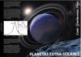
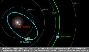
Figure 1: Visualizing extra-solar planets from their position distribution, as it might be seen from telescope.

As explained by Aime and Soummer (2004) the complex amplitude of a wave in the focal plane of a telescope, at a position $(x,y)$, can be written as follows:

$$\psi(x,y)=C(x,y)+S(x,y),$$

where $C(x,y)\in\mathbb{C}$ is a deterministic term proportional to the wave amplitude in absence of turbulence and $S(x,y)\in\mathbb{C}$ is the wavefront amplitude (associated to the speckles) distributed according to a zero mean complex Gaussian distribution. Tourneret et al. (2005) assumed that the telescope aperture has central symmetries which imply $C(x,y)\in\mathbb{R}$ and using the fact that the real and imaginary parts of $\psi(x,y)$, denoted by $\psi_{r}(x,y)$ and $\psi_{i}(x,y)$ have Gaussian distributions, extended the instantaneous intensity of the wave in the focal plane at a position $(x,y)$, given by

$$\Lambda(x,y)=|\psi(x,y)|^{2}=\psi_{r}(x,y)^{2}+\psi_{i}(x,y)^{2}$$

to multidimensional case. They demonstrated that

$$\boldsymbol{\Lambda}=(\Lambda(1),\ldots,\Lambda(n^{2}))^{T}=\psi_{r}\psi_{r}^{T}+\psi_{i}\psi_{i}^{T},$$

where $\psi_{r}=(\psi_{r}(1),\ldots,\psi_{r}(n^{2}))^{T}$ and $\psi_{r}=(\psi_{i}(1),\ldots,\psi_{i}(n^{2}))^{T}$, has non-central Wishart distribution.

Since speckles are bigger than they appear in telescope, it is highly misleading to assume the normality assumption, even if the assumption of symmetry is taken, to study of planet formation. See Figure 2 for the distribution of amplitude of wave in the focal plane of a telescope.

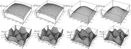
Figure 2: Instantaneous intensity of the wave in the focal plane.

Thus it is more plausible to take these speckles as extremes in amplitude of a wave or outlier in plane formation as appears in telescope. In conclusion, accepting the assumption of symmetry, the multivariate t-distribution (or may be lighter tail alternative to Gaussian, as it might be captured from Figure 2) is a relevant alternative to the normal one. Hence, by the theory discussed in the above, $\boldsymbol{\Lambda}=(\Lambda(1),\ldots,\Lambda(n^{2}))^{T}$ has non-central GW distribution arises from taking $g$ to be the kernel of multivariate t-distribution in Eq. (2).

7 Conclusion

In this paper a family of distributions were introduced from the Wishart generator distribution which includes the Wishart as a special case. The Wishart generator distribution might be important for a number of practical signal processing applications including synthetic aperture radar (SAR), multi-antenna wireless communications and direct imaging of extra-solar planets, the latter was discussed using the non-central Wishart generator distribution. Several statistical properties of this newly defined distribution were studied from matrix theory viewpoint. Brief notes regarding classical as well as Bayesian estimations were also proposed.

8 Appendix

Initially let $\mathcal{S}_{m}$ and $\mathcal{I}_{m}$ be the spaces of all positive definite matrices of order $m$ and all symmetric matrices between 0 and $\boldsymbol{I}_{m}$ under the meaning of partial Löwner ordering, respectively. For a given matrix $\boldsymbol{A}\in\mathbb{R}^{p\times p}$, $\boldsymbol{A}^{T}$ denotes the transpose of $\boldsymbol{A}$, $\mathop{\mathrm{t}r}\nolimits(\boldsymbol{A})=a_{11}+\ldots+a_{pp}$; $\mathop{\mathrm{e}tr}\nolimits(\boldsymbol{A})=\exp(\mathop{\mathrm{t}r}\nolimits(\boldsymbol{A}))$; $\det(\boldsymbol{A})=$ determinant of $\boldsymbol{A}$; norm of $\boldsymbol{A}=\|\boldsymbol{A}\|=$ maximum of absolute values of latent roots of the matrix $\boldsymbol{A}$; and $\boldsymbol{A}^{\frac{1}{2}}$ denotes the unique square root of $\boldsymbol{A}$.

Also denote the space of all orthogonal matrices of order $m$ by

$$\mathcal{O}(m)=\left\{\boldsymbol{H}|\boldsymbol{H}^{\prime}\boldsymbol{H}=\boldsymbol{I}_{m},\boldsymbol{H}\boldsymbol{H}^{\prime}=\boldsymbol{I}_{m}\right\},\quad\int_{\mathcal{O}(m)}\textnormal{d}\boldsymbol{H}=1.$$

Let $k$ be a positive integer; a partition $\kappa$ of $k$ is written as $\kappa=(k_{1},k_{2},\ldots)$, where $\sum_{r}k_{t}=k$.

Definition 5

(Muirhead, 2005) Let $\boldsymbol{Y}$ be an $m\times m$ symmetric matrix with latent roots $y_{1},\cdots,y_{m}$ and let $\kappa=(k_{1},\cdots,k_{m})$ be a partition of $k$ into not more than $m$ parts. The zonal polynomial of $\boldsymbol{Y}$ corresponding to $\kappa$, denoted by $C_{\kappa}(\boldsymbol{Y})$, is a symmetric, homogeneous polynomial of degree $k$ in the latent roots $y_{1},\cdots,y_{m}$ such that:

1. The term of highest weight in $C_{\kappa}(\boldsymbol{Y})$ is $y_{1}^{k_{1}},\cdots y_{m}^{k_{m}}$; that is,
   (1)  $C_{\kappa}(\boldsymbol{Y})=d_{k}y_{1}^{k_{1}},\cdots y_{m}^{k_{m}}$+terms of lower weight,
   where $d_{k}$ is a constant.

2. $C_{\kappa}(\boldsymbol{Y})$ is an eigenfunction of the differential operator $\triangle_{\boldsymbol{Y}}$ given by
   (2)  $\triangle_{\boldsymbol{Y}}=\sum_{i=1}^{m}y_{i}^{2}\frac{\partial^{2}}{\partial y_{i}^{2}}+\sum_{i=1}^{m}\sum_{j=1,j\neq i}^{m}\frac{y_{i}^{2}}{y_{i}-y_{j}}\;\frac{\partial}{\partial y_{i}}$.
   

3. As $\kappa$ varies over all partitions of $k$ the zonal polynomial have unit coefficients in the expansion of $(tr\boldsymbol{Y})^{k}$; that is,
   (3)  $(tr\boldsymbol{Y})^{k}=(y_{1}+\cdots+y_{m})^{k}=\sum_{\kappa}C_{\kappa}(\boldsymbol{Y})$.

Immediate consequence of Definition 5 is the following important equality

$$\mathop{\mathrm{e}tr}\nolimits(\boldsymbol{X})=\sum_{k=0}^{\infty}\frac{\mathop{\mathrm{t}r}\nolimits(\boldsymbol{X})^{k}}{k!}=\sum_{k=0}^{\infty}\sum_{\kappa}\frac{C_{\kappa}(\boldsymbol{X})}{k!}.$$ (35)

Let $\boldsymbol{X},\boldsymbol{Y}\in\mathbb{C}^{m\times m}$ then

$$C_{\kappa}(\boldsymbol{X})C_{\tau}(\boldsymbol{Y})=\sum_{\phi\in\kappa\cdot\tau}\theta_{\phi}^{\kappa,\tau}C_{\phi}^{\kappa,\tau}(\boldsymbol{X},\boldsymbol{Y})$$ (36)

where $\theta_{\phi}^{\kappa,\tau}=\frac{C_{\phi}^{\kappa,\tau}(\boldsymbol{I}_{m},\boldsymbol{I}_{m})}{C_{\phi}(\boldsymbol{I}_{m})}$.

For any $\boldsymbol{X},\boldsymbol{Y}\in\mathcal{S}_{m}$, we have (Gross and Richards, 1987)

$$\int_{\mathcal{O}(m)}C_{\kappa}(\boldsymbol{X}\boldsymbol{H}\boldsymbol{Y}\boldsymbol{H}^{\prime})\textnormal{d}\boldsymbol{H}=\frac{C_{\kappa}(\boldsymbol{X})C_{\kappa}(\boldsymbol{Y})}{C_{\kappa}(\boldsymbol{I}_{m})}.$$

For any $\boldsymbol{A}\in\mathcal{S}_{m}$, we have (Gross and Richards, 1987)

$$\int_{0<\boldsymbol{X}<\boldsymbol{I}_{m}}\det(\boldsymbol{X})^{a-\frac{1}{2}(m+1)}C_{\kappa}(\boldsymbol{A}\boldsymbol{X})\textnormal{d}\boldsymbol{X}=\frac{\left(a\right)_{\kappa}B_{m}\left(a,\frac{1}{2}(m+1)\right)}{\left(a+\frac{1}{2}(m+1)\right)_{\kappa}}C_{\kappa}(\boldsymbol{A}).$$

Let $a_{1},\ldots,a_{p}$ and $b_{1},\ldots,b_{q}$ be complex numbers, such that for $1\leq i\leq p$ and $1\leq j\leq q$, $b_{i}>(j-1)/2$. Then the hypergeometric function of one matrix argument is defined as

$${}_{p}F_{q}(a_{1},\ldots,a_{p};b_{1},\ldots,b_{q};\boldsymbol{X})=\sum_{k=0}^{\infty}\sum_{\kappa}\frac{(a_{1})_{\kappa},\ldots,(a_{p})_{\kappa}}{(b_{1})_{\kappa},\ldots,(b_{q})_{\kappa}}\frac{C_{\kappa}(\boldsymbol{X})}{k!},$$

where $\sum_{\kappa}$ denotes the summation over all partition $\kappa$, $\kappa=(k_{1},\ldots,k_{m})$, $k_{1}\geq k_{2}\geq\ldots\geq 0$, of $k$, and the generalized hypergeometric coefficient $(b)_{\kappa}$ is given by

$$(b)_{\kappa}=\prod_{i=1}^{m}\left(b-\frac{1}{2}(i-1)\right)_{k_{i}},\quad(b)_{k}=b(b+1)\ldots(b+k-1),\quad(b)_{0}=1.$$

The multivariate gamma function which is frequently used alongside is defined as

$$\Gamma_{m}(a)=\int_{\mathcal{S}_{m}}\det(\boldsymbol{X})^{a-\frac{1}{2}(m+1)}\mathop{\mathrm{e}tr}\nolimits(-\boldsymbol{X})\textnormal{d}\boldsymbol{X}=\pi^{\frac{1}{4}m(m-1)}\prod_{i=1}^{m}\Gamma\left(a-\frac{1}{2}(i-1)\right),$$

where $\mathop{\mathrm{R}e}\nolimits(a)>(m-1)/2$.

Multivariate beta function is defined as

$$B_{m}(a,b)=\int_{\mathcal{I}_{m}}\det(\boldsymbol{X})^{a-\frac{1}{2}(m+1)}\det(\boldsymbol{I}_{m}-\boldsymbol{X})^{b-\frac{1}{2}(m+1)}\textnormal{d}\boldsymbol{X}=\frac{\Gamma_{m}(a)\Gamma_{m}(b)}{\Gamma_{m}(a+b)},$$

where $\mathop{\mathrm{R}e}\nolimits(a),\mathop{\mathrm{R}e}\nolimits(b)>(m-1)/2$.

Definition 6

The Laplace transform of the matrix valued function $f$ is given by

$$g(\boldsymbol{Y})=\mathcal{L}_{f}(\boldsymbol{X})=\int_{\mathcal{S}_{m}}\mathop{\mathrm{e}tr}\nolimits(-\boldsymbol{X}\boldsymbol{Y})f(\boldsymbol{X})\textnormal{d}\boldsymbol{X}$$ (37)

Definition 7

(Press, 1982) A random matrix $\boldsymbol{V}\in\mathcal{S}_{m}$ is said to have the non-singular Wishart distribution with scale matrix $\boldsymbol{\Sigma}\in\mathcal{S}_{m}$ and $n$ degrees of freedom, $m\leq n$, if the joint distribution of the distinct elements of $\boldsymbol{V}$ is continues with density

$$f(\boldsymbol{V}) = c\det(\boldsymbol{\Sigma})^{-\frac{1}{2}n}\det(\boldsymbol{V})^{\frac{1}{2}(n-m-1)}\mathop{\mathrm{e}tr}\nolimits\left[-\frac{1}{2}\boldsymbol{\Sigma}^{-1}\boldsymbol{V}\right],$$

where $c^{-1}=2^{\frac{mn}{2}}\Gamma_{m}\left(\frac{n}{2}\right)$. It is denoted by $\boldsymbol{V}\sim W_{m}(\boldsymbol{\Sigma},n)$.

Further if we take $\boldsymbol{U}=\boldsymbol{V}^{-1}$, then $\boldsymbol{U}$ follows the inverted Wishart distribution with scale matrix $\boldsymbol{\Sigma}$ and $n$ degrees of freedom denoted by $\boldsymbol{U}\sim IW_{m}(\boldsymbol{\Sigma},n)$ with the following density

$$g(\boldsymbol{U}) = c\det(\boldsymbol{\Sigma})^{\frac{1}{2}n}\det(\boldsymbol{U})^{-\frac{1}{2}n-\frac{1}{2}(m+1)}\mathop{\mathrm{e}tr}\nolimits\left[-\frac{1}{2}\boldsymbol{\Sigma}\boldsymbol{U}^{-1}\right].$$

Lemma 15

(Teng et al., 1989) Assume $\boldsymbol{Z}$ is an $m\times m$ symmetric matrix, $\boldsymbol{X}$ is an $m\times m$ complex symmetric matrix with $\mathop{\mathrm{R}e}\nolimits(\boldsymbol{X})\in\mathcal{S}_{m}$ and $h$ is a real function over $\mathbb{R}^{+}$. Then

$$\int_{\mathcal{S}_{m}}\det(\boldsymbol{W})^{a-\frac{1}{2}(m+1)}C_{\kappa}(\boldsymbol{W}\boldsymbol{Z})h(\mathop{\mathrm{t}r}\nolimits\boldsymbol{X}\boldsymbol{W})\textnormal{d}\boldsymbol{W}=\frac{(a)_{\kappa}\Gamma_{m}(a)\gamma_{k}(a)}{\Gamma(am+k)}\;\det(\boldsymbol{X})^{-a}C_{\kappa}(\boldsymbol{Z}\boldsymbol{X}^{-1}),$$

where $\mathop{\mathrm{R}e}\nolimits(a)>(m-1)/2$ and

$$\gamma_{k}(a)=\int_{\mathbb{R}^{+}}y^{am+k-1}h(y)\textnormal{d}y.$$ (38)

9 Acknowledgements

We would hereby acknowledge the support of the StatDisT group. We would also want to thank Prof. Srivastava (University of Toronto) for his help in Theorem 14. This work is based upon research supported by the UP Vice-chancellor’s post-doctoral fellowship programme.

10 References

A. Y. Abul-Magd, G. Akemann and P. Vivo, Superstatistical generalizations of Wishart Laguerre ensembles of random matrices, J. Phys. A: Math. Theo., 42 (2009), 175-207.

S. Adhikari, Generalized Wishart distribution for probabilistic structural dynamics, Comp. Mech., 45 (2010), 495-511.

C. Aime and R. Soummer, Influence of speckle and Poisson noise on exoplanet detection with a coronograph, in EUSIPCO-04 (L. Torres, E. Masgrau, and M. A. Lagunas, eds.), (Vienna, Austria), (2004), 509-512.

T. W. Anderson, An Introduction to Multivariate Statistical Analysis, 3rd Edition, John Wiley, New York, (2003).

T. W. Anderson and K. T. Fang, On the theory of multivariate elliptically contoured distributions and their applications, Technical Report, No. 54, Department of Statistics, Stanford University, California, (1979).

M. Arashi, A. K. Md. Ehsanes Saleh, Daya K. Nagar, S. M. M. Tabatabaey and H. Salarzadeh Jenatabadi, Bayesian Statistical Inference For Laplacian Class of Matrix Variate Elliptically Contoured Models, Comm. Statist. Theo. Meth., Accepted (2013).

W. Bryc, Compound real Wishart and q-Wishart matrices, arXiv:0806.4014v1 [math.PR] (2008).

José A. Díaz-García, Ramón Gutiérrez-Jáimez, On Wishart distribution: Some extensions, J. Lin. Alg. 435 (2011), 1296-1310.

A. P. Dawid, and S. L. Lauritzen, Hyper-Markov laws in the statistical analysis of decomposable graphical models. Ann. Statist. 21 (1993), 1272-317.

J. Fan, Non-central Cochran’s theorem for elliptically contoured distributions, Acta Math. Sinica, 3(2) (1986), 185-198.

G. Frahm, Generalized Elliptical Distributions: Theory and Applications, PhD Dissertation, Universität zu Köln, (2004).

Francisco J. Caro-Lopera, Graciela González-Farías, N. Balakrishnan, On generalized Wishart distributions - I: Likelihood ratio test for homogeneity of covariance matrices, Sankhya A, DOI 10.1007/s13171-013-0047-7, (2014).

E. D. Feigelson and G. J. Babu, Modern Statistical Methods for Astronomy With R Applications, Cambridge, UK, (2012).

A. K. Gupta and D. K. Nagar, Matrix variate distributions Chapman & Hall/CRC, (2000).

I. S. Gradshteyn and I. M. Ryzhik, Table of Integrals, Series, and Products, 7th Ed., Academic Press, USA, (2007).

K. I. Gross and D. ST. P. Richards, Special functions of matrix argument I: Algebraic induction zonal polynomials and hypergeometric functions, Trans. Amer. Math. Soc., 301 (1987), 475 501.

Anis Iranmanesh, M. Arashi, D. K. Nagar and S. M. M. Tabatabaey, On Inverted Matrix Variate Gamma Distribution, Comm. Statist. Theo. Meth., 42(1) (2013), 28-41.

G. Letac and H. Massam, The normal quasi-Wishart distribution. In: Viana MAG, Richards DStP (eds) Algebraic Methods in Statistics and Probability. AMS Contemp Math 287 (2001), 231 239.

E. Lukacs, and R. G. Laha, Applications of Characteristic Functions, Griffin s Statistical Monographs & Courses, 14. Charles Griffin & Co., Ltd., London, (1964).

Rob J. Muirhead, Aspect of Multivariate Statistical Theory, 2nd Ed., John Wiley, New York, (2005).

S. Munilla and R. J. C. Cantet, Bayesian conjugate analysis using a generalized inverted Wishart distribution accounts for differential uncertainty among the genetic parameters an application to the maternal animal model, J. Anim. Breed. Genet., 129 (2012), 173 187.

S. J. Press, Applied Multivariate Analysis, Holt, Rinchart & Winston, New York, (1982).

A. Roverato, Hyper-Inverse Wishart Distribution for Non- decomposable Graphs and its Application to Bayesian Inference for Gaussian Graphical Models, Scandinavian J. Statist., 29 (2002), 391-411.

M. S. Srivastava and C. G. Khatri, An Introduction to Multivariate Analysis, North-Holland, Amsterdam, (1979).

B. C. Sutradhar, and M. M. Ali, A generalization of the Wishart distribution for the elliptical model and its moments for the multivariate t model, J. Mult. Anal., 29 (1989), 155-162.

C. Teng, H. Fang, W. Deng, The generalized noncentral Wishart distribution, L. Math. Res. Exp., 9(4) (1989), 479-488.

J. Y. Tourneret, A. Ferrari, G. Letac, The noncentral Wishart distribution: Properties and application to speckle imaging, in: Proc. IEEE Workshop on Stat. Signal Proc., (2005), 1856 1860

H. Wang and M. West, Bayesian analysis of matrix normal graphical models, Biometrika, 96(4) (2009), 821-834.

C. S. Withers and S. Nadarajah, log det A = tr log A, Int. J. Math. Education Sci. Tech., 41(8) (2010), 1121-1124

C. S. Wong, T. Wang, Laplace-Wishart distributions and Cochran theorems, Sankhya 57 (1995), 342-359.