Trapped-ion Lissajous trajectories

Abstract

Here we present a protocol for generating Lissajous curves with a trapped ion by engineering Rashba- and the Dresselhaus-type spin-orbit interactions in a Paul trap. The unique anisotropic Rashba $\alpha_{x}$, $\alpha_{y}$ and Dresselhaus $\beta_{x}$, $\beta_{y}$ couplings afforded by our setup also enables us to obtain an “unusual” Zitterbewegung, i.e., the semiconductor analog of the relativistic trembling motion of electrons, with cycloidal trajectories in the absence of magnetic fields. We have also introduced bounded SO interactions, confined to an upper-bound vibrational subspace of the Fock states, as an additional mechanism to manipulate the Lissajous motion of the trapped ion. Finally, we accounted for dissipative effects on the vibrational degrees of freedom of the ion and find that the Lissajous trajectories are still robust and well defined for realistic parameters.

Increasing interest in quantum simulations and controllable trapped ion systems —used through the last two decades as a staging platform to investigate fundamental quantum phenomena FP and to implement quantum information processing QI — have led to the emulation of the quantum relativistic wave equation. Apart from trapped ions Solano ; Bermudez , a number of distinct setups have been used to simulate zitterbewegung in a variety of physical systems such as quantum wells Loss , photonic crystals Zhang , Bose-Einstein condensates Spielman and ultracold atoms Vaishnav . It has been demonstrated that Bose-Einstein condensates can provide an analog to sonic black holes Zoller and the Higgs boson HB .

In trapped-ion system Gerritsma et al. Blatt reported a proof-of-principle quantum simulation of the one-dimensional Dirac equation within a trapped-ion experiment. Measuring the time-evolving position of a single trapped ion set to mathematically simulate a free relativistic quantum particle, they demonstrated the Dirac Zitterbewegung, as anticipated in Ref. Solano , for distinct initial superpositions of positive- and negative-energy spinor-like states. The momentum-spin coupling, which naturally takes place in the relativistic quantum regime, was simulated by the laser-induced coupling between the vibrational and the electronic states of the ion.

Motivated by the exciting results in Refs. Blatt ; Solano , here we consider a single two-level atom in a two-dimensional Paul trap with four electrodes, Fig.1, and show how to obtain spin-orbit interactions of the Rashba and Dresselhaus types, ubiquitous in quantum spintronics and in emerging areas of condensed matter physics such as topological insulators and Majorana fermions. Our setup enables us to engineer Hamiltonians with anisotropic SO couplings such as

$$H_{SO}=\frac{\alpha_{x}}{\hbar}\sigma_{x}p_{y}-\frac{\alpha_{y}}{\hbar}\sigma_{y}p_{x}+\frac{\beta_{x}}{\hbar}\sigma_{x}p_{x}+\frac{\beta_{y}}{\hbar}\sigma_{y}p_{y},$$ (1)

which generalize the canonical form of the SO interactions in semiconductor quantum wells to include distinct Rashba $\alpha_{x}$, $\alpha_{y}$ and Dresselhaus $\beta_{x}$, $\beta_{y}$ couplings. In (1) $\vec{p}$ and $\vec{\sigma}$ denote the momentum and pseudo-spin operators, respectively, of the trapped ion. Interestingly, the anisotropic SO couplings can give rise to physical phenomena not possible in the condensed matter environment, e.g., ionic motion with trajectories following Lissajous curves, Fig.1. In Fig. 2 we show the whole set of Lissajous curves followed by the trapped ion, which we discuss in detail below. In addition, we can also obtain the “unusual” Zitterbewegung, a trembling relativistic motion, with cycloidal trajectories in the absence of magnetic fields Ze . We also demonstrate how to engineer bounded-SO Hamiltonians, confined to an upper-bound vibrational subspace of the Fock states —leading to distincts periodic motions— apart from analysing the effects of dissipation over trajectories.

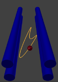
Figure 1: The schematic of the experimental Paul trap setup illustrating the ion performing a Lissajous curve.

Engineering the anisotropic Rashba interaction. We consider a two-level ion acted upon by two laser beams perpendicular to one another in $x$ and $y$ directions, each providing red and blue sidebands simultaneously via an electro-optical modulator Sackett . From the four generated frequencies $\omega_{\ell}$ and relative phases $\phi_{\ell}$, two are tuned to the first-blue sidebands, each coming from one of the original laser beams. The other two are tuned to the first-red sidebands, leading to the Hamiltonian ($\hbar=1$)

$$H =i\left[\Omega_{x}\eta_{x}\left(e^{i\phi_{1}}a_{x}+e^{i\phi_{2}}a_{x}^{\dagger}\right)\right.$$

$$\left.+\Omega_{y}\eta_{y}\left(e^{i\phi_{3}}a_{y}+e^{i\phi_{4}}a_{y}^{\dagger}\right)\sigma_{+}+H.c.\right]\text{,}$$ (2)

where $\eta_{\alpha}$ is the Lamb-Dicke parameter and $\Omega_{\emph{s}}$ the Rabi frequency for the coupling between the electronic (ground $\left|g\right\rangle$ and excited $\left|e\right\rangle$) states of the ion and its two-dimensional motional degrees of freedom, described by the annihilation $a_{\emph{s}}$ and creation $a_{\emph{s}}^{\dagger}$ operators with respect to each direction $\emph{s}=x$,$y$. Moreover, $\sigma_{+}=\left|e\right\rangle\left\langle g\right|$ and $\sigma_{-}=\sigma_{+}^{\dagger}$ are the raising and lowering operators for the two-level system. By adjusting $\phi_{1}=0,\phi_{2}=\pi,\phi_{3}=\pi/2$, and $\phi_{4}=3\pi/2$, we obtain, in the interaction picture, the anisotropic 2D Rashba SO interaction

$$H=\left(\Delta_{x}\eta_{x}\Omega_{x}p_{x}\sigma_{y}-\Delta_{y}\eta_{y}\Omega_{y}p_{y}\sigma_{x}\right)\text{,}$$ (3)

where $p_{\emph{s}}=i\left(a_{\emph{s}}^{\dagger}-a_{\emph{s}}\right)/2\Delta_{\emph{s}}$, with $\Delta_{\emph{s}}$ $=1/\sqrt{2m\nu_{\emph{s}}}$, $m$ being the ion mass and $\nu_{\emph{s}}$ the trap frequency in the s direction. When we adjust the laser parameters so that $\Delta_{x}=\Delta_{y}$, $\eta_{x}=\eta_{y}$, and $\Omega_{x}=\Omega_{y}$, the above derived Hamiltonian reduces exactly to the usual Rashba interaction $H=\gamma\left(p_{x}\sigma_{y}-p_{y}\sigma_{x}\right)$ in quantum wells, where $\gamma=\Delta\eta\Omega$.

Interestingly, we find that a 3D trap with an additional laser beam and an appropriate set of phase constants $\phi_{\ell}$ enables us to engineer a 3D Rashba-like term

$$H=\gamma\hat{r}.\left(\vec{p}\times\vec{\sigma}\right)\text{,}$$ (4)

where $\vec{r}$ sets the position of the ion in relation to the trap center. Unlike the 2D and 3D cases in Eqs. (3) and (4), the 1D Rashba-like interaction $H=\gamma p_{x}\sigma_{y}$ does not lead to the unusual Zitterbewegung with cycloidal orbits. However, when one of the original laser beams leading to Eq. (2) is adjusted to produce a carrier interaction (instead of the simultaneous red and blue sidebands), we end up with the 1D interaction

$$H=\gamma p_{x}\sigma_{y}+\tilde{\Omega}\sigma_{z}\text{.}$$ (5)

Here, as in the Dirac equation, the energy gap provided by the Stark shift term $\tilde{\Omega}\sigma_{z}$ ($\tilde{\Omega}$ being also a Rabi frequency), is a key ingredient for producing Zitterbewegung. In addition, an appropriate choice of parameters of the laser producing simultaneous blue and red sidebands leads straightforwardly to a Hamiltonian similar to that in Eq. (5): $H=\eta\Omega\Delta_{x}$ $p_{x}\sigma_{x}+\tilde{\Omega}\sigma_{z}$, which simulates the 1D Dirac equation Solano .

Anisotropic Dresselhaus term. We can also simulate the linear Dresselhaus SO interaction by adjusting $\phi_{1}=-\phi_{2}=\pi/2$ and $\phi_{3}=-\phi_{4}=3\pi/2$ in Eq. (2); we find

$$H=\gamma\left(p_{x}\sigma_{x}-p_{y}\sigma_{y}\right)\text{,}$$ (6)

which, together with the Rashba coupling, is a crucial ingredient to manipulate the electron spin in quantum spintronics and, more recently, to obtain exotic topological phases of matter. We can also consider four laser beams simultaneously and hence generate a Rashba-Dresselhaus Hamiltonian as shown in Eq. (1), with $\alpha_{\emph{s}}=\Delta_{\emph{s}}\eta_{\emph{s}}\Omega_{\emph{s}}$ and $\beta_{\emph{s}}=\Delta_{\emph{s}}\tilde{\eta}_{\emph{s}}\tilde{\Omega}_{\emph{s}}$, enabling us to simulate the canonical SO interaction of quantum spintronic in our setup.

At this point it is important to stress that a four-level ion, as in Ref. Solano , can also be used to engineer the interactions of the forms [Eqs. (1)– (6)]. In this case we have to consider two additional states $\left|g^{\prime}\right\rangle$ and $\left|e^{\prime}\right\rangle$ having the same angular momentum as $\left|g\right\rangle$ and $\left|e\right\rangle$, respectively, but distinct energies and magnetic momenta. For instance, by exciting only the crossed transitions $g\leftrightarrow e^{\prime}$ and $e\leftrightarrow g^{\prime}$, we can exactly simulate the mathematical structure of the Hamiltonian used to obtain the unusual zitterbewegung in Ref. Ze . In this case, the isotropic Rashba-type interaction (3) is modified to

$$H=\tilde{\sigma}_{x}\otimes\Gamma\left(p_{x}\sigma_{y}-p_{y}\sigma_{x}\right)\text{,}$$ (7)

where $\Gamma=\Delta\eta\Omega$ and $\tilde{\sigma}_{x}$ is the Pauli matrix in subspace $\left\{\left|g^{\prime}\right\rangle,\left|e^{\prime}\right\rangle\right\}$. All other Hamiltonians [Eqs. (1) – (6)] are also modified via a tensor products with $\tilde{\sigma}_{x}$. For simplicity, we restrict our analysis to a two-level system which, as shown below, gives rise to the same dynamics for the unusual Zitterbewegung as given in Ref. Ze .

“Bounded” spin orbit interaction. Before analyzing the Lissajous curves in Fig. 2, we would like to address a case, with no analog in the solid state physics, in which an upper-bound interaction ToAppear between the internal and the vibrational degrees of freedom of the ion is engineered. Following the steps outlined in Ref. ToAppear , we can obtain

$$H_{k=\pm 1}=\chi(\eta)\left[\mathbf{A}(\eta)\sigma_{\pm}+\mathbf{A}^{\dagger}(\eta)\sigma_{\mp}\right]\text{,}$$ (8)

where $\chi(\eta)=\eta\left(1-\eta^{2}/2\right)\Omega e^{i\phi}$ and $\mathbf{A}(\eta)=\left[1-\eta^{2}a^{\dagger}a/2\right]a$. Expanding the operators $A$ and $A^{\dagger}$ in the Fock space basis and adjusting the Lamb-Dicke parameter to $\eta^{2}=2/N$ $\left[\eta^{2}=2/\left(N-1\right)\text{ with }N\in\mathbb{Z}\right]$ such that $\mathbf{A}^{\dagger}(\eta)\left|N\right\rangle=0$ $\left[\mathbf{A}(\eta)\left|N\right\rangle=0\right]$, we find that for an initial vribational state prepared within the upper-bound subspace ranging from $\left|0\right\rangle$ to $\left|N\right\rangle$, the Hamiltonian $H_{k=\pm 1}$ becomes

$$H_{\pm}^{(ub)}={\displaystyle\sum\limits_{n=0}^{N-1}}\chi_{n}\left(\left|n\right\rangle\left\langle n+1\right|\sigma_{\pm}+H.c.\right).$$ (9)

where $\chi_{n}=\sqrt{n+1}\left(1-\eta^{2}n/2\right)\chi(\eta)$. By using the Hamiltonian (1) instead of (2) we can derive all the above spin-orbit interactions but restricted to within the upper-bound subspace. In particular, for the case of the upper-bound Rashba-Dresselhaus interaction, with the same adjustment of the laser parameters as above we obtain

$$H=\alpha_{x}p_{x}^{ub}\sigma_{y}-\alpha_{y}p_{y}^{ub}\sigma_{x}+\beta_{x}p_{x}^{ub}\sigma_{x}-\beta_{y}p_{y}^{ub}\sigma_{y}\text{,}$$ (10)

where $p_{\emph{s}}^{ub}=i\left[\mathbf{A}_{\emph{s}}^{\dagger}(\eta)-\mathbf{A}_{\emph{s}}(\eta)\right]/2\Delta_{\emph{s}}$, $\alpha_{\emph{s}}=\chi_{n}\eta\Delta_{\emph{s}}$, and $\beta_{\emph{s}}=\tilde{\chi}_{n}\eta\Delta_{\emph{s}}$. As should become clearer below, when discussing the trajectories, the bounded Hamiltonian (10) is able to generate Lissajous trajectories other than those derived from the usual Rashba-Dresselhaus interaction. It also enables Lissajous curves from an initial coherent state, which does not occur with interaction (1). We finally note that for each upper-bound parameter $N$ we get distincts trajectories.

Cycloidal Zitterbewegung. Now let us analyze the zitterbewegung with the (anisotropic) Rashba-like coupling in Eq. (3), from which we obtain the time-dependent components of position operator

$$\emph{s}(t)=\emph{s}(0)-\frac{c^{2}P_{\emph{s}}}{H}t-iH\left(c\sigma_{\emph{r}}+\frac{c^{2}P_{\emph{s}}}{H}\right)\left(e^{iHt}-1\right)\text{,}$$ (11)

with $\emph{r}\neq\emph{s}=x,y$. We note that Eq. (11) exhibits the same time dependence as that coming from the Dirac zitterbewegung, with the trembling motion arising from the third term on the right side of the equality. Hereafter we consider the initial state $\left|\psi(0)\right\rangle={\textstyle\prod\nolimits_{\emph{s}}}\exp\left[-(p_{\emph{s}}-p_{0\emph{s}})/2\mu_{\emph{s}}\right]\otimes\left|\varphi\right\rangle$, with both momentum eigenstates peaked around $p_{0\emph{s}}$ ($\mu_{\emph{s}}$ being the width of the distribution) and $\left|\varphi\right\rangle$ standing for the ionic internal state, we thus compute the mean value $\left\langle\bar{s}(\tau)\right\rangle=\operatorname*{Tr}\left[\bar{s}\rho(t)\right]$:

$$\left\langle\bar{s}(\tau)\right\rangle =\left\langle\bar{s}(0)\right\rangle+\left(-1\right)^{1+\delta_{\emph{s}x}}\varepsilon^{\delta_{\emph{s}y}}\left\langle\sigma_{\emph{r}}\right\rangle\tau$$

$$+\frac{\varepsilon\bar{p}_{\emph{r}}}{2\xi}\left[\cos\left(2\xi^{1/2}\tau\right)-1\right]\left\langle\sigma_{z}\right\rangle$$

$$+\frac{\varepsilon\bar{p}_{\emph{r}}}{2\xi^{3/2}}\left[\sin\left(2\xi^{1/2}\tau\right)-2\xi^{1/2}\tau\right]$$

$$\times\left(\left\langle\sigma_{x}\right\rangle\bar{p}_{x}+\varepsilon\left\langle\sigma_{y}\right\rangle\bar{p}_{y}\right)$$ (12)

where we have defined the dimensionless position $\bar{s}=s/\Delta$, momentum $\bar{p}_{\emph{s}}=2\Delta p_{\emph{s}}$ and time $\tau=\eta\Omega t$, with $\xi=\sqrt{\left\langle\bar{p}_{\emph{s}}^{2}\right\rangle+\left\langle\bar{p}_{\emph{r}}^{2}\right\rangle}$ and $\varepsilon=\Delta_{x}^{2}\eta_{x}\Omega_{x}/\Delta_{y}^{2}\eta_{y}\Omega_{y}$. Here $\delta_{\emph{s}x}$ is the Kronecker delta and $\varepsilon=1$ ($\neq 1$) gives the isotropic (anisotropic) Rashba-type interaction. We take the momentum state to be a distribution in the $x$ direction with $\varepsilon^{2}\bar{p}_{y}^{2}\gg\bar{p}_{x}^{2}$ and the vacuum state in the $y$ direction. With the internal state $\left|\varphi\right\rangle=\left|a\right|\left|\uparrow\right\rangle+\left|b\right|\operatorname*{e}\nolimits^{i\phi}\left|\downarrow\right\rangle$, where $\left|a\right|\neq\left|b\right|$ and $\phi=\pi/2$, such that $\left\langle\sigma_{x}\right\rangle=0$, we obtain

$$\left\langle\bar{x}(\tau)\right\rangle =\left(\frac{\varepsilon^{2}\bar{p}_{y}^{2}}{2\bar{p}_{x}^{2}}-1\right)\tau-\frac{\varepsilon^{2}\bar{p}_{y}^{2}}{2\bar{p}_{x}^{3}}\left[\sin\left(2\bar{p}_{x}\tau\right)\right]\text{,}$$ (13a)

$$\left\langle\bar{y}(\tau)\right\rangle =\frac{\varepsilon\bar{p}_{x}}{2\xi}\left[\cos\left(2\bar{p}_{x}\tau\right)-1\right]\text{.}$$ (13b)

The above equations lead to all the trochoids in Ref. Ze , for appropriate parameters.

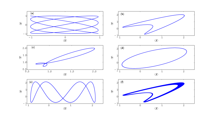
Figure 2: (a) Lissajou curves derived from Eq. (17) with $\varpi=1.96$ and $\eta\Omega\varpi$ and $\eta\Omega\sqrt{\varpi}$ around $50$ and $35$ KHz, respectively. (b) Lissajous curves numerically computed from Eq. (10), starting from initial coherent state $\Theta=1$ and electronic levels in the superposition $\left|\varphi\right\rangle=\left|\uparrow\right\rangle-i\left|\downarrow\right\rangle$, with $N=1$ and $\gamma_{\emph{s}}/\Delta_{\emph{s}}=1$. In (c) and (d) we consider the same parameters as in (b), except for (c) $\Theta=1-i$ and (d) $N=2$. In (e) we consider the same initial states as in (b) but $N=2$, $\gamma_{x}/\Delta_{x}=0.4$ and $\gamma_{y}/\Delta_{y}=1$. Finally, (f) follows from the same parameters as in (b) but considering dissipative mechanisms in the vibrational degrees of freedom, with a damping rate $\zeta_{\emph{s}}=10^{-4}\gamma_{\emph{s}}/\Delta_{\emph{s}}$.

When considering the Dresselhaus-type interaction (6) we obtain exactly the same time dependence as in Eq. (12) but with $\left\langle\sigma_{x}\right\rangle\bar{p}_{x}+\varepsilon\left\langle\sigma_{y}\right\rangle\bar{p}_{y}$ changed by $\left\langle\sigma_{x}\right\rangle\bar{p}_{y}+\varepsilon\left\langle\sigma_{y}\right\rangle\bar{p}_{x}$, affecting only the amplitude of the curves generated by Eq. (12). This ensures that the cycloidal trajectories without magnetic fields, derived in Ref. (Ze ) by considering the effects of an interband SO term, can also be obtained here from the anisotropic Dresselhaus interaction. However, when the Rashba- and the Dresselhaus-type interactions come together as in Eq. (1), we obtain for the isotropic case ($\alpha_{x}=\alpha_{y}$ and $\beta_{x}=\beta_{y}$)

$$\left\langle\bar{s}(\tau)\right\rangle =\left\langle\bar{s}(0)\right\rangle+\left[\left(-1\right)^{1+\delta_{sx}}\left(\left\langle\sigma_{s}\right\rangle-\kappa\left\langle\sigma_{r}\right\rangle\right)\right]\tau$$

$$-\kappa_{s}\varkappa^{-2}\left\langle\bar{p}_{r}\right\rangle\left\langle\sigma_{z}\right\rangle\left[1-\cos\left(\varkappa\tau\right)\right]$$

$$-\kappa_{s}\varkappa^{-3}\left\langle\bar{p}_{r}\right\rangle\mathcal{\Lambda}\left[\sin\left(\varkappa\tau\right)-\tau\right]$$ (14)

where we have defined the dimensionless coupling $\kappa=\alpha/\beta$, and the parameters $\kappa_{\emph{s}}=2\left(\kappa^{2}+\left(-1\right)^{1+\delta\emph{s}y}\right)$, $\varkappa=2\kappa\left[\kappa\xi^{2}+2\left\langle\bar{p}_{x}\bar{p}_{y}\right\rangle\right]$, and $\Lambda=\left\langle\left(\kappa\bar{p}_{y}+\bar{p}_{x}\right)\sigma_{y}+\left(\kappa\bar{p}_{x}+\bar{p}_{y}\right)\sigma_{x}\right\rangle$. Equation (14) shows that with both spin-orbit couplings acting together with different strengths ($\kappa\neq 1$), we still obtain similar trajectories to those coming from each coupling acting separately. Now, when considering matched coupling strenghts ($\kappa=1$, i.e., $\alpha=\beta$), two special situations arise when the electronic levels are prepared as eigenstates of $\sigma_{z}$ or $\sigma_{\emph{s}}$. In the first case we do not get Zitterbewegung as expected, since an eigenstate of $\sigma_{z}$ does not simulate the superposition between positive and negative energy states required for the Zitterbewegung. However, we do obtain an interesting effect: we lock the motion of the particle in the s direction and obtain an oscillatory harmonic motion in the r direction:

$$\left\langle\bar{s}(\tau)\right\rangle =\left\langle\bar{s}(0)\right\rangle-\kappa_{s}\varkappa^{-2}\left\langle\bar{p}_{\emph{r}}\right\rangle\text{,}$$ (15a)

$$\left\langle\bar{r}(\tau)\right\rangle =\left\langle\bar{r}(0)\right\rangle-\kappa_{r}\varkappa^{-2}\left\langle\bar{p}_{s}\right\rangle\left[1-\cos\left(\varkappa\tau\right)\right]\text{.}$$ (15b)

In the second case we get a uniform motion in the s direction and the expected trembling motion in the r direction:

$$\left\langle\bar{s}(\tau)\right\rangle =\left\langle\bar{s}(0)\right\rangle+\left(-1\right)^{1+\delta_{sx}}\left\langle\sigma_{s}\right\rangle\tau\text{,}$$ (16a)

$$\left\langle\bar{r}(\tau)\right\rangle =\left\langle\bar{r}(0)\right\rangle+\left(-1\right)^{1+\delta_{sx}}\tau$$

$$-\kappa_{r}\varkappa^{-3}\left\langle\bar{p}_{s}\right\rangle\left\langle\bar{p}_{y}+\bar{p}_{x}\right\rangle\left[\sin\left(\varkappa\tau\right)-\tau\right]\text{.}$$ (16b)

Although Eq. (16b) does not lead to trajectories similar to those discussed in Ref. Ze , we note that Eq. (14) can have its parameters properly adjusted  so as to produce cycloidal motion..

Ionic Lissajous trajectories. Now we revisit the anisotropic version of the Rashba-type Hamiltonian (6), $H=\left(\gamma_{x}p_{x}\sigma_{x}-\gamma_{y}p_{y}\sigma_{y}\right)$. By adjusting the laser fields such that $\gamma_{y}^{2}\gg\gamma_{x}^{2}$ and preparing the electronic state as an eigenstate of $\sigma_{z}$, we obtain

$$\left\langle\bar{s}(\tau)\right\rangle =\left\langle\bar{s}(0)\right\rangle-\left\langle\bar{p}_{r}\right\rangle\left[1-\cos\left(\varpi\tau\right)\right]\text{,}$$ (17a)

$$\left\langle\bar{r}(\tau)\right\rangle =\left\langle\bar{r}(0)\right\rangle+\left\langle\bar{p}_{s}\bar{p}_{r}^{-1}\right\rangle\left[1-\cos\left(\sqrt{\varpi}\tau\right)\right]\text{,}$$ (17b)

with $$\varpi=\left(\gamma_{x}/\gamma_{y}\right)\left\langle\bar{p}_{y}\right\rangle \varpi=1.96 \eta\Omega\varpi \eta\Omega\sqrt{\varpi} 50 35 \gamma\sqrt{\bar{p}_{x}+\bar{p}_{x}} 10^{-10} \left|\Theta\right\rangle \left|\psi(0)\right\rangle N=1, \gamma_{\emph{s}}/\Delta_{\emph{s}}=1 \Theta=1 \left|\varphi\right\rangle=\left|\uparrow\right\rangle-i\left|\downarrow\right\rangle \Theta=1-i N=2 N=2 \gamma_{x}/\Delta_{x}=0.4 \gamma_{y}/\Delta_{y}=1$$. In Fig. 2(a) we show Lissajous curves governed by Eq. (17) with and frequencies and around and KHz, respectively. In this case, the Rashba energy is around eV. In what follows we obtain Lissajous figures from our previously introduced bounded SO interaction in Eq. (10), which requires only the preparation of an initial vibrational coherent state (differently from all the equations of motion derived above, which rely on the preparation of the initial vibrational state ). In Fig. 2(b) the mean value of the ionic position has been numerically computed (running in QuTiP QuTIP ) from Eq. (10), with , and starting from the vibrational mode in the coherent state and electronic levels in the superposition . In Figs. 2(c) and 2(d) we consider the same parameters as in Fig. 2(b) except for in Fig. 2(c) and in Fig. 2(d). In Fig. 2(e) we consider , , , and the same initial states as in Fig. 2(b).

Detrimental effects. To show that our calculated ionic trajectories are robust, we have included damping effects due to the environment. Figure 2(f) is similar (same parameters) to in Fig.2(b) but accounts for dissipative mechanisms in the vibrational degrees of freedom as described by the Lindbladian $(\zeta_{\emph{s}}/2)\left[2a_{\emph{s}}\rho a_{\emph{s}}^{\dagger}-a_{\emph{s}}^{\dagger}a_{\emph{s}}\rho-\rho a_{\emph{s}}^{\dagger}a_{\emph{s}}\right]$, with a damping rate $\zeta_{\emph{s}}=10^{-4}\gamma_{\emph{s}}/\Delta_{\emph{s}}$ exp . Clearly, the trajectories are robust and visible for realistic parameters.

We have presented a protocol for generating Lissajous curves with the vibrational motion of an ion in a two-dimensional trap. It relies on the unique capability of our setup to realize Rashba- and Dresselhaus-type SO interactions, which allows us to simulate solid-state SO effects within a highly controllable trapped-ion experiment. We have also verified that Lissajous curves can be derived from upper-bound SO interactions, which may bring new perspectives to the subject. Addressing some interesting issues to be investigated further, we first observe that a straightforward extension to the case of many trapped ions, where the strong and tunable (up to $10^{4}Hz$) SO strength can be used to explore quantum phase transitions QPT and chaotic behavior chaos . Finally, motivated by the results above, we believe it is worth to investigate the role of the “Bounded” spin orbit interaction in solid states systems s1 .

Acknowledgements

The authors acknowledge financial support from PRP/USP within the Research Support Center Initiative (NAP Q-NANO) and FAPESP, CNPQ and CAPES, the Brazilian agencies.

References

(1)C. Monroe et al., Science 272, 1131 (1995); Q.
A. Turchette et al., Phys. Rev. Lett. 81, 3631 (1998); C. J.
Myatt et al., Nature 403, 269 (2000); M. A. Rowe et al.,
Nature 409, 791 (2001); M. D. Barrett et al., Nature
429 (2004); D. Leibfried et al., Nature 438, 639
(2005); D. J. Wineland, Rev. Mod. Phys. 75, 4714 (2013).
(2)C. Monroe et al., Phys. Rev. Lett. 75, 4714
(1995); D. Kielpinski et al., Nature 417, 709 (2002); J.
Chiaverini et al., Nature 432, 602 (2004); J. P. Home et
al., Science 325, 1227 (2009); C. Ospelkaus et al., Nature
476, 181 (2011); J. P. Gaebler, et al., Phys. Rev. Lett.
109, 179902 (2012).
(3)L. Lamata et al., Phys. Rev. Lett. 98,
253005 (2007).
(4)A. Bermudez et al., Phys. Rev. A 76,
041801(R) (2007).
(5)Schliemann et al., Phys. Rev. Lett. 94,
266801 (2005).
(6)X. Zhang, Phys. Rev. Lett. 100, 113903 (2008).
(7)Y.-J. Lin, K. Jiménez-García, and I. B. Spielman,
Nature 471, 83 (2011).
(8)J. Y. Vaishnaw et al., Phys. Rev. Lett.
100, 153002 (2008).
(9)L. J. Garay et al., Phys. Rev. Lett. 85,
4643 (2000).
(10)K. Hamilton et al., JHEP 10, 222 (2013); F.-J.
Huang,Q.-H. Chen,W.-M. Liu, arXiv:1207.3707v3 [cond-mat.quant-gas] (2013).
(11)R. Gerritsma et al., Nature 463, 68 (2010).
(12)E. Bernardes et al., Phys. Rev. Lett. 99,
076603 (2007).
(13)C. A. Sackett et al., Nature (London) 404,
256 (2000).
(14)R. F. Rossetti et al., Phys. Rev. A 90,
033840 (2014).
(15)J. R. Johansson, P. D. Nation, and F. Nori, Comput. Phys.
Commun. 183, 1760 (2012); ibid. 184, 1234 (2013).
(16)D. Leibfried et al., Rev. Mod. Phys. 75, 281 (2003).
(17)Y. Zhang, G. Chen, and C. Zhang, Sci. Rep. 3, 1937 (2013).
(18)J. Larson, B. M. Anderson, and A. Altland; Phys. Rev. A
87, 013624 (2013).
(19)I. Zutic, J. Fabian and S. Das Sarma, Rev. Mod. Phys.
76, 323 (2004).