Automata and Graph Compression

Abstract

We present a theoretical framework for the compression of automata, which are widely used in speech processing and other natural language processing tasks. The framework extends to graph compression. Similar to stationary ergodic processes, we formulate a probabilistic process of graph and automata generation that captures real world phenomena and provide a universal compression scheme LZA for this probabilistic model. Further, we show that LZA significantly outperforms other compression techniques such as gzip and the UNIX compress command for several synthetic and real data sets.

1 Introduction

The rapid generation of data by search engines and popular online sites, which has been reported to be in the order of hundreds of petabytes, requires efficient storage mechanisms and better compression algorithms. Similarly, sophisticated models on mobile devices for tasks such as speech-to-text conversion often need large storage space and memory constraints on these devices demand better compression algorithms. Furthermore, downloading these models requires high bandwidth so transmitting a compressed version saves communication costs. Hence there is a need for efficient data compression both at the data warehouse level (petabytes of data) and at a device level (megabytes of data).

Most of the current compression techniques have been developed for sequential data. For example, Huffman coding and arithmetic coding are optimal compression schemes when the underlying sequence is distributed independently (i.i.d.) according to some known distribution [10]. If the sequence is not generated according to an i.i.d. process, but generated from a stationary ergodic process, then Lempel-Ziv schemes are asymptotically optimal [21, 16]. In practice, a combination of these schemes are often used. For example, the UNIX compress command implements Lempel-Ziv-Walsh (LZW) and gzip combines Lempel-Ziv-77 (LZ77) and Huffman coding.

However, data is often structured. For example, in a webgraph, a node represents a URL and a directed edge between two nodes indicates that one URL has a link to another. In social networks, a node represents a user and an edge between two nodes indicates that they are friends. Finite automata and transducers are widely used in speech recognition, and a variety of other language processing tasks such as machine translation, information extraction, and parsing [18]. For example, in speech-processing automata, a path may correspond to a possible sentence in a language model or in a set of recognizer hypotheses (a so-called lattice). Often these data sets are very large. For web graphs, there are tens of billions of web pages to choose from. For speech processing, a large-alphabet language model may have billions of word edges. Hence structured data compression is useful in practice.

A natural question is to ask how one can exploit the structure in data to develop better compression algorithms? Can one do better than serializing the data and applying algorithms for sequence compression? Surprisingly, these questions and the compression of structured data have received little attention. Motivated by previous examples, we focus on automata compression and, as a corollary, graph compression.

[6, 15, 5] studied webgraph compression empirically. Theoretical webgraph compression was first studied by [1] who proposed a scheme that uses a minimum spanning tree to find similar nodes to compress. However, they showed that many generalizations of their problem are NP hard. Motivated by probabilistic models, [8, 9] showed that arithmetic coding can be used to near-optimally compress (the structure of) graphs generated by the Erdős-Rényi model.

Automata compression empirically has been studied by [11, 12, 13]. However, we are not aware of any theoretical work focused on automata compression. Our goal is three-fold: $(i)$ propose a probabilistic model for automata that captures real world phenomena, $(ii)$ provide a provable universal compression algorithm, and $(iii)$ show experimentally that the algorithm fares well compared to techniques such as gzip and compress. We note that our probabilistic model can be viewed as a generalization of Erdős-Rényi graphs [4].

The rest of the paper is organized as follows: in Section 2, we describe automata and their properties. In Section 3, we describe our probabilistic model and show how it captures many real-world applications. In Section 4, we describe our proposed algorithm LZA, prove its optimality and in Section 5, we demonstrate the algorithm’s practicality in terms of its degree of compression.

2 Directed Graphs and Finite Automata

A directed graph is a pair $(Q,\delta)$ where $Q=\{1,2,3,\ldots,n\}$ is the set of nodes and $\delta\colon Q\rightarrow Q^{*}$ is the set of edges where for every node $q$, $\delta(q)$ is the set of nodes to which it is connected. Note that our notation for directed graphs is chosen to harmonize with finite automata.

Automata generalize graphs. An unweighted automaton $A$ is a $5$-tuple $(Q,\Sigma,\delta,q_{i},F)$ where $Q=\{1,2,\ldots,n\}$ is the set of states, $\Sigma=\{1,2,\ldots,m\}$ is a finite alphabet, $\delta\colon Q\times\Sigma\rightarrow Q^{*}$ is the transition function, $q_{i}\in Q$ is the initial state, and $F\subseteq Q$ are the final states. The transitions from state $q$ by label $a$ to states $\{q^{\prime}_{1},q^{\prime}_{2},\ldots\}$ are given by $\delta(q,a)=\{q^{\prime}_{1},q^{\prime}_{2},\ldots\}$. If there is no transition by label $a$, then $\delta(q,a)=\emptyset$. We use $E\subset Q\times\Sigma\times Q$ to denote the set of all transitions $(q,a,q^{\prime})$ and $E[q]$ to denote the set of all transitions from state $q$.

Figure 1: An example automaton.

Figure 2: A subway turnstile automaton.

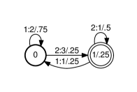
Figure 3: An example weighted transducer.

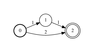
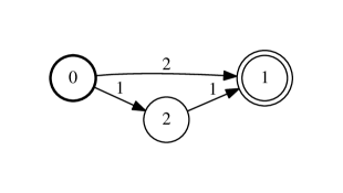
Figure 4: An example of isomorphic automata. The above two automata are same under the permutation $0\to 0,1\to 2$, and $2\to 1$

An example of an automaton is given in Figure 2. State 0 in this simple example is the initial state (depicted with the bold circle) and state 1 is the final state (depicted with double circle). The strings 12 and 222 are among those accepted by this automaton. By using symbolic labels on this automaton in place of the usual integers, as depicted in Figure 2, we can interpret this automaton as the operation of a subway turnstile. It has two states locked and unlocked and actions (alphabet) coin and push. If the turnstile is in the locked state and you push, it remains locked and if you insert a coin, it becomes unlocked. If it is unlocked and you insert a coin it remains unlocked, but if you push once it becomes locked.

Note that directed graphs form a subset of automata with $\Sigma=\{1\}$ and hence we focus on automata compression. Furthermore, to be consistent with the existing automata literature, we use states to refer to nodes and transitions to refer to edges in both graphs and automata going forward.

A main motivation to study automata is their application in speech and natural language processing. In some circumstances, transitions may be generalized to have an output label and a weight as well as the usual input label. Such automata, called weighted finite state transducers (FSTs), are extensively used in these fields [19, 18, 2]. An example of an FST is given in Figure 3. The string 12 is among those accepted by this transducer. For this input, the transducer outputs the string 23 and has weight $.046875$ (transitions weights $0.75$ times $0.25$ times final weight $0.25$).

We propose an algorithm for unweighted automata compression. For FSTs, we use the same algorithm by treating the input-output label pair as a single label. If the automaton is weighted, we just add the weights at the end of the compressed file by using some standard representation.

3 Random automata compression

3.1 Probabilistic model

Our goal is to propose a probabilistic model for automata generation that captures real world phenomena. To this end, we first review probabilistic models on sequences and draw connections to probabilistic models for automata.

3.1.1 Probabilistic processes on sequences

We now define i.i.d. sampling of sequences. Let $x^{n}_{1}$ denote an $n$-length sequence $x_{1},x_{2}\ldots x_{n}$. If $x^{n}_{1}$ are $n$ independent samples from a distribution $p$ over ${\cal X}$, then $p(x^{n}_{1})=\prod^{n}_{i=1}p(x_{i})$. Note that under i.i.d. sampling, the index of the sample has no importance, i.e.,

$$p(X_{i}=x)=p(X_{j}=x),\,\forall 1\leq i,j\leq n,x\in{\cal X}.$$

stationary ergodic processes generalizes i.i.d. sampling. For a stationary ergodic process $p$ over sequences

$$p(X^{m}_{i}=x^{m}_{i})=p(X^{m+j}_{i+j}=x^{m}_{i}),\forall i,j,m,x^{m}_{i}.$$

Informally stationary ergodic processes are those for which only the relative position of the indices matter and not the actual ones.

3.1.2 Probabilistic processes on automata

Before deriving models for automata generation, we first discuss an invariance property of automata that is useful in practice. The set of strings accepted by an automaton and the time and space of its use are not affected by the state numbering. Two automata are isomorphic if they coincide modulo a renumbering of the states. Thus, automata $(Q,\Sigma,\delta,q_{i},F)$ and $(Q^{\prime},\Sigma,\delta^{\prime},q^{\prime}_{i},F^{\prime})$ are isomorphic, if there is a one-to-one mapping $f\colon Q\to Q^{\prime}$ such that $f(\delta(q,a))=\delta^{\prime}(f(q),a)$, for all $q\in Q$ and $a\in\Sigma$, $f(q_{i})=q^{\prime}_{i}$, and $f(F)=F^{\prime}$, where $f(F)=\{f(q)\colon q\in F\}$.

Under stationary ergodic processes, two sequences with the same order of observed symbols have the same probabilities. Similarly we wish to construct a probabilistic model of automata such that any two isomorphic automata have the same probabilities, since the state numbering does not have explicit importance, For example, the probabilities of automata in Figure 4 are the same.

There are several probabilistic models of automata and graphs that satisfy this property. Perhaps the most studied random model is the Erdős-Rényi model $G(n,p)$, where each state is connected to every other state independently with probability $p$ [4]. Note that if two automata are isomorphic then the  Erdős-Rényi model assigns them the same probability. The Erdős-Rényi model is analogous to i.i.d. sampling on sequences. We wish to generalize the Erdős-Rényi model to more realistic models of automata.

Since the state numbering is to be disregarded, the only possible dependence of transitions from a state would be by the paths leading to that state. This arises naturally in language modeling tasks. For example in an $n$-gram model, a state might have an outgoing transition with label Francisco or Diego only if it has a input transition with label San. This is an example where we have restrictions on paths of length $2$. In general, we may have restrictions on paths of any length $\ell$.

We define an $\ell$-memory model for automata as follows. Let $h^{\ell}_{q}$ be the set of paths of length at most $\ell$ leading to the state $q$. The probability distribution of transitions from a state depends on the paths leading to it. Let $\delta(q,*)\stackrel{{\scriptstyle\mathrm{def}}}{{=}}\delta(q,1),\delta(q,2),\ldots,\delta(q,m)$.

$$p(A) =p(\delta(1,*),\delta(2,*),\ldots,\delta(n,*))\propto\prod^{n}_{q=1}p(\delta(q,*)|h^{\ell}_{q}).$$

Similarly, transitions leaving a state $q$ dissociate into marginals conditioned on the history $h^{\ell}_{q}$ and probability that $q^{\prime}\in\delta(q,a)$ also dissociates into marginals.

$$p(\delta(q,*)|h^{\ell}_{q}) =\prod_{a\in\Sigma}p(\delta(q,a)|h^{\ell}_{q})$$

$$=\prod_{a\in\Sigma}\prod^{n}_{q^{\prime}=1}p(\mathbb{I}(q^{\prime}\in\delta(q,a))|h^{\ell}_{q}),$$

where $\mathbb{I}(q^{\prime}\in\delta(q,a))$ is the indicator of the event $q^{\prime}\in\delta(q,a)$. Note that the probabilities are defined with proportionality. This is due to the probabilities possibly not adding to one. Thus we have a constant $Z$ to ensure that it is a probability distribution.

$$p(A) =p(\delta(1,*),\delta(2,*),\ldots,\delta(n,*))$$

$$=\frac{1}{Z}\prod^{n}_{q=1}p(\delta(q,*)|h^{\ell}_{q})$$

$$=\frac{1}{Z}\prod^{n}_{q=1}\prod_{a\in\Sigma}p(\delta(q,a)|h^{\ell}_{q}).$$

Note that $\ell$-memory models assign the same probability to automata that are isomorphic. In our calculations, we restrict $\ell$ to make the model tractable.

Note that sequences form a subset of automata as follows. For a sequence $x^{n}$ over alphabet $\Sigma$, consider the automata representation with states $Q=\{1,2,\ldots n\}$, initial state $q_{i}=1$, final state $F=\{n\}$, alphabet $\Sigma$, and transition function $\delta(i,x_{i})=i+1$ and $\delta(i,x)=\phi$ for all $x\neq x_{i}$. Informally, every sequence can be represented as an automaton with line as the underlying structure. Furthermore, note that the probability that two isomorphic automata should have the same probability is same as stating the indices in sequences do not have explicit meaning (stationary ergodic property).

3.2 Entropy and coding schemes

A compression scheme is a mapping from $\mathcal{X}$ to $\{0,1\}^{*}$ such that the resulting code is prefix-free and can be uniquely recovered. For a coding scheme $c$, let $l_{c}(x)$ denote the length of the code for $x\in{\cal X}$. It is well-known that the expected number of bits used by any coding scheme is the entropy of the distribution, defined as $H(p)\stackrel{{\scriptstyle\mathrm{def}}}{{=}}\sum_{x\in{\cal X}}p(x)\log\frac{1}{p(x)}$. The well known Huffman coding scheme achieves this entropy up-to one additional bit. For $n$-length sequences arithmetic coding is used, which achieves compression up-to entropy with few additional bits of error.

The above-mentioned coding methods such as Huffman coding and arithmetic coding require the knowledge of the underlying distribution. In many practical scenarios, the underlying distribution may be unknown and only the broader class to which the distribution belongs may be known. For example, we might know that the given $n$-length sequence is generated by i.i.d. sampling of some unknown distribution $p$ over $\{1,2,\ldots,k\}$. The objective of a universal compression scheme is to asymptotically achieve $H(p)$ bits per symbol even if the distribution is unknown. A coding scheme $c$ for sequences over a class of distributions ${\cal P}$ is called universal if

$$\limsup_{n\to\infty}\max_{p\in{\cal P}}\frac{\mathbb{E}[l_{c}(X^{n})]-H(X^{n})}{n}=0.$$

The normalization factor in the above definition is $n$, as the number of sequences of length $n$ increases linearly with $n$. For automata and graphs with $n$ states (denoted by $A_{n}$) we choose a scaling scaling factor of $n^{2}$ as the number of automata scales as $\exp(n^{2})$. We call a coding scheme $c$ for automata over a class of distributions ${\cal P}$ universal if

$$\limsup_{n\to\infty}\max_{p\in{\cal P}}\frac{\mathbb{E}[l_{c}(A_{n})]-H(A_{n})}{n^{2}}=0.$$

We now describe the algorithm LZA. Note that the algorithm does not require the knowledge of the underlying parameters or the probabilistic model.

4 Algorithm for automaton compression

Our algorithm recursively finds substructures over states and uses a Lempel-Ziv subroutine. Our coding method is based on two auxiliary techniques to improve the compression rate: Elias-delta coding and coding the differences. We briefly discuss these techniques and their properties before describing our algorithm.

4.1 Elias-delta coding and coding the differences

Elias-delta coding is a universal compression scheme for integers [14]. To represent a positive integer $x$, Elias-delta codes use $\lfloor\log x\rfloor+2\lfloor\log\lfloor\log x\rfloor+1\rfloor+1$ bits. To obtain a code over $\mathbb{N}\cup\{0\}$, we replace $x$ by $x+1$and use Elias-delta codes.

We now use Elias-delta codes to obtain to code sets of integers. Let $x_{1},x_{2},\ldots,x_{m}$ be integers such that $0\leq x_{1}\leq x_{2}\leq\cdots\leq x_{m}\leq n$. We use the following algorithm to code $x_{1},x_{2},\ldots,x_{m}$. The decoding algorithm follows from Elias-decode [14].

Algorithm Difference-Encode
Input: Integers $0\leq x_{1}\leq x_{2}\leq\cdots\leq x_{m}\leq n$. 1. Use Elias-encode to code $x_{1}-0$, $x_{2}-x_{1}$, …$x_{d}-x_{d-1}$.

Lemma 1 (Appendix A).

For integers such that $0\leq x_{1}\leq x_{2},\ldots x_{d}\leq n$, Difference-Encode uses at most

$$d\log\frac{n+d}{d}+2d\log\Bigl{(}\log\frac{n+d}{d}+1\Bigr{)}+d$$

bits.

We first give an example to illustrate Difference-Encode’s usefulness. Consider graph representation using adjacency lists. For every source state, the order in which the destination states are stored does not matter. For example, if state $1$ is connected to states $2$, $4$, and $3$, it suffices to represent the unordered set $\{2,3,4\}$. In general if a state is connected to $d$ out of $n$ states, then it suffices to encode the ordered set of states $y_{1},y_{2},\ldots,y_{d}$ where $1\leq y_{1}\leq y_{2}\leq y_{3}\ldots y_{d}\leq n$. The number of such possible sets is $\binom{n}{d}$. If the state-sets are all equally likely, then the entropy of state-sets is $\log{n\choose d}\approx d\log\frac{n}{d}$.

If each state is represented using $\log n$ bits, then $d\log n>d\log\frac{n}{d}$ bits are necessary, which is not optimal. However, by Lemma 1, Difference-Encode uses $d\log\frac{n+d}{d}(1+o(1))\approx d\log\frac{n}{d}$, and hence is asymptotically optimal. Furthermore, the bounds in Lemma 1 are for the worst-case scenario and in practice Difference-Encode yields much higher savings. A similar scenario arises in LZA as discussed later.

4.2 LZA

We now have at our disposal the tools needed to design a variant of the Lempel-Ziv algorithm for compressing automata, which we denote by LZA. Let $d_{q}\stackrel{{\scriptstyle\mathrm{def}}}{{=}}|E[q]|$ be the number of transitions from state $q$ and let transitions in $E[q]=\{(q,a_{1},q_{1}),(q,a_{2},q_{2}),\ldots,(q,a_{d_{q}},q_{d_{q}})\}$ are ordered as follows: for all $i$, $q_{i}\leq q_{i+1}$ and if $q_{i}=q_{i+1}$ then $a_{i}<a_{i+1}$.

The algorithm is based on the observation that the ordering of the transitions leaving a state does not affect the definition of an automaton and works as follows. The states of the automaton are visited in a BFS order. For each state visited, the set of outgoing transitions are sorted based on their destination state. Next, the algorithm recursively finds the largest overlap of the sets of transitions that match some dictionary element and encodes the pair (matched dictionary element number, next transition), and adds the dictionary element to $T_{d}$, alphabet of the transition to $T_{\Sigma}$, and the transition to $T_{\delta}$. It also updates the dictionary element by adding a new dictionary element (matched dictionary element number, next transition) to the dictionary. Finally it encodes $T_{d}$, $T_{\delta}$ using Difference-Encode and encodes each element in $T_{\Sigma}$ using $\lceil\log m\rceil$ bits.

Algorithm LZA 
Input: The transition label function $\delta$ of the automaton. Output: Encoded sequence $S$. 1. Set dictionary $D=\emptyset$. 2. Visit all states $q$ in BFS order. For every state $q$ do: (a) Code $d_{q}$ using $\lceil\log nm\rceil$ bits. (b) Set $T_{d}=\emptyset$, $T_{\Sigma}=\emptyset$, and $T_{\delta}=\emptyset$. (c) Start with $j=1$ in $E[q]=\{(q,a_{1},q_{1}),(q,a_{2},q_{2}),\ldots,(q,a_{d_{q}},q_{d_{q}})\}$ and continue till $j$ reaches $d_{q}$. i. Find largest $l$ such that $(a_{j},q_{j}),\ldots,(a_{j+l},q_{j+l})\in D$. Let this dictionary element be $d_{r}$. ii. Add $(a_{j},q_{j}),\ldots,(a_{j+l+1},q_{j+l+1})$ to $D$. iii. Add $d_{r}$ to $T_{d}$, $q_{j+l+1}$ to $T_{\delta}$, and $a_{j+l+1}$ to $T_{\Sigma}$. (d) Use Difference-Encode to encode $T_{d}$, $T_{\delta}$ and encode each element in $T_{\Sigma}$ using $\lceil\log m\rceil$ bits. Append these sequences to $S$ 3. Discard the dictionary and output $S$.

We note that simply compressing the unordered sets $T_{d}$ and $T_{\delta}$ suffices for unique reconstruction and thus Difference-Encode is the natural choice. Observe that Difference-Encode is a succinct representation of the dictionary and does not affect the way Lempel-Ziv dictionary is built. Thus the decoding algorithm follows immediately from retracing the steps in LZA and LZ78 decoding algorithm.

If Difference-Encode is not used, the number of bits used would be approximately $|D|\log|D|+|D|\log n$, which is strictly greater than that number of bits in Lemma 2. Furthermore, we did consider several other natural variants of this algorithm where we difference-encode the states first and then serialize the data using a standard Lempel-Ziv algorithm. However, we could not prove asymptotic optimality for those variants. Proving their non-optimality requires constructing distributions for which the algorithm is non-optimal and is not the focus of this paper.

We first bound the number of bits used by LZA in terms of the size of the dictionary $|D|$, the number of states $n$, and the alphabet size $m$. This bound is independent of the underlying probabilistic model. Next, we proceed to derive probabilistic bounds.

Lemma 2 (Appendix B).

The total number of bits used by LZA is at most

$$|D|\left[\log(n+1)+\log\left(\nu+1\right)+2\log(\log(n+1)+1)\right]+|D|\left[2\log\left(\log\left(\nu+1\right)+1\right)+2+\lceil\log m\rceil\right]+n\lceil\log nm\rceil,$$

where $\nu=\frac{n^{2}}{|D|}$.

4.3 Proof of optimality

In this section, we prove that LZA is asymptotically optimal for the random automata model introduced in Section 3. Lemma 2 gives an upper bound on the number of bits used in terms of the size of the dictionary $|D|$. We now present a lower bound on the entropy in terms of $D$ which will help us prove this result. The proof is given in Appendix C.

Lemma 3.

LZA satisfies

$$H(p)\geq\mathbb{E}[|D|]\left[\log\frac{\mathbb{E}[|D|]}{n}-m^{\ell}-\log\left(\frac{n^{2}m}{\mathbb{E}[|D|]}+1\right)-1\right].$$

The above result together with Lemma 2 implies

Theorem 4 (Appendix D).

If $2^{m^{\ell}}=o\left(\frac{\log n}{\log\log n}\right)$, then LZA is a universal compression algorithm.

5 Experiments

5.1 Automaton structure compression

LZA compresses automata, but for most applications, it is sufficient to compress the automata structure. We convert LZA into LZA_S, an algorithm for automata structure compression as follows. We first perform a breadth first search (BFS) with the initial state as the root state and relabel the states in their BFS visitation order. We then run LZA with the following modification. In step $2$, for every state $q$ we divide the transitions from $q$ into two groups, $T^{q}_{\text{old}}$ transitions whose destination states have been traversed before in LZA and $T^{q}_{\text{new}}$, transitions whose destinations have not been traversed. Note that since the state numbers are ordered based on a BFS visit, the destination state numbers in $T^{q}_{\text{new}}$ are $1,2,\ldots n$, and can be recovered easily while decoding and thus need not be stored. Hence, we run step $2b$ in LZA only on transitions in $T^{q}_{\text{old}}$. For $T^{q}_{\text{new}}$, we just compress the transition labels using LZ78.

Since each destination state can appear in $T^{q}_{\text{new}}$ only once, the number of transitions in $\cup_{q}T^{q}_{\text{new}}\leq n$, Since this number is $\ll n^{2}$, the normalization factor in the definition of universal compression algorithm for automata, the proof of Theorem 4 extends to LZA_s. Since for most applications, it is sufficient to compress to the automata structure, we implemented LZA_s in C++ and added it to the OpenFst open-source library [3].

5.2 Comparison

The best known convergence rates of all Lempel-Ziv algorithms for sequences are ${\cal O}\left(\frac{\log\log n}{\log n}\right)$ and LZA has the same convergence rate under the $\ell$-memory probabilistic model.

However in practice data sets have finitely many states and the underlying automata may not be generated from an $\ell$-memory probabilistic model. To prove the practicality of the algorithm, we compare LZA_s with the Unix compress command (LZ78) and gzip (Lempel-Ziv-Walsh and Huffman coding) for various synthetic and real data sets.

5.2.1 Synthetic Data

While the $\ell$-memory probabilistic model illustrates a broad class of probabilistic models on which LZA is universal, generating samples from an $\ell$-memory model is difficult as the normalization factor $Z$ is hard to compute. We therefore test our algorithm on a few simpler synthetic data sets. In all our experiments the number of states is $1000$ and the results are averaged over $1000$ runs.

Table 1 summarizes our results for a few synthetic data sets, specified in bytes. Note that one of the main advantages of LZA_S over existing algorithms is that LZA_S just compresses the structure, which is sufficient for applications in speech processing and language modeling. Furthermore, note that to obtain the actual automaton from the structure we need the original state numbering, which can be specified in $n\log n$ bits, which is less than $1250$ bytes in our experiments. Even if we add $1250$ bits to our results in Table 1, LZA still performs better than gzip and compress.

We run the algorithm on four different synthetic data sets $G_{1},G_{2},A_{1},A_{2}$. $G_{1}$ and $A_{1}$ are models with a uniform out-degree distribution over the states and $G_{2}$ and $A_{2}$ are models with a non-uniform out-degree distribution:
$G_{1}$: directed Erdős-Rényi graphs where we randomly generate transitions between every source-destination pair with probability $1/100$.
$A_{1}$: automata version of Erdős-Rényi graphs, where there is a transition between every two states with probability $1/100$ and the transition labels are chosen independently from an alphabet of size $10$ for each transition.
$G_{2}$: We first assign each state a class $c\in\{1,2,\ldots 1000\}$ randomly. We connect every two states $s$ and $d$ with probability $1/(c_{s}+c_{d})$. This ensures that the graph has degrees varying from $2$ to $\log 1000$.
$A_{2}$: we generate the transitions as above and we label each transition to be a deterministic function of the destination state. This is similar to $n$-gram models, where the the destination state determines the label. Here again we chose $|\Sigma|=10$.

Class	LZAS	compress	gzip	LZA$+$gzip
$G_{1}$	$18260$	$22681$	$23752$	$17320$
$A_{1}$	$21745$	$33478$	$31682$	$21108$
$G_{2}$	$2536$	$4994$	$4564$	$2443$
$A_{2}$	$3027$	$6707$	$5546$	$2940$

Table 1: Synthetic data compression examples (in bytes).

Note that LZA always performs better than the standard Lempel-Ziv-based algorithms gzip and compress. Note that algorithms designed with specific knowledge of the underlying model can achieve better performance. For example, for $G_{1}$, arithmetic coding can be used to obtain a compressed file size of $n^{2}h(0.01)/8\approx 10000$ bytes. However the same algorithm would not perform well for $G_{2}$ or $A_{2}$.

5.2.2 Real-World Data

We also tested our compression algorithm on a variety of ‘real-world’ automata drawn from various speech and natural language applications. These include large speech recognition language models and decoder graphs [18], text normalization grammars for text-to-speech [20], speech recognition and machine translation lattices [17], and pair $n$-gram grapheme-to-phoneme models [7]. We selected approximately eighty such automata from these tasks and removed their weights and output labels (if any), since we focus here on unweighted automata. Figure 5 shows the compressed sizes of these automata, ordered by their uncompressed (adjacency-list) size rank, with the same set of compression algorithms presented in the synthetic case. At the smallest sizes, gzip out-performs LZA, but after about 100 kbytes in compressed size, LZA is better. Overall, the combination of LZA and gzip performs best.

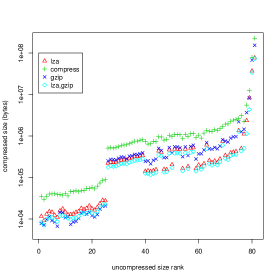
Figure 5: Real-world compression examples.

6 Acknowledgements

We thank Jayadev Acharya and Alon Orlitsky for helpful discussions.

Appendix A Proof of Lemma 1

Since $0$ is included in the set, the number of bits used to represent $x$ is upper bounded by $\theta(x)=\log(x+1)+2\log(\log(x+1)+1)\rfloor+1$. Observe that $\theta$ is a concave function since both $\log$ and $x\mapsto\log(\log x)$ are concave. Let $x_{0}=0$. Then, by the concavity of $\theta$, the total number of bits $B$ used can be bounded as follows:

$$B \leq\sum_{i=1}^{d}\theta(x_{i}-x_{i-1})$$

$$=d\,\sum_{i=1}^{d}\frac{1}{d}\theta(x_{i}-x_{i-1})$$

$$\leq d\,\theta\Big{(}\frac{1}{d}\sum_{i=1}^{d}x_{i}-x_{i-1}\Big{)}=d\,\theta\Big{(}\frac{1}{d}x_{n}\Big{)}\leq d\,\theta\Big{(}\frac{n}{d}\Big{)},$$

where we used for the last inequality $x_{n}\leq n$ and the fact that $\theta$ is an increasing function. This completes the proof of the lemma.

Appendix B Proof of Lemma 2

Let $k_{q}$ be the number of elements added to the dictionary when state $q$ is visited by LZA. The maximum value of the destination state is $n$. Thus, by Lemma 1, the number of bits used to code $T_{\delta}$ is at most

$$\sum_{q=1}^{n}\Big{(}k_{q}\theta\Big{(}\frac{n}{k_{q}}\Big{)}+k_{q}\lceil\log m\rceil\Big{)},$$

where $\theta(\cdot)$ is the function introduced in the proof of Lemma 1. Similarly, since the maximum value of any dictionary element is $|D|$, by Lemma 1, the number of bits used to code $T_{d}$ is at most

$$\sum_{q=1}^{n}k_{q}\theta\bigg{(}\frac{|D|}{k_{q}}\bigg{)}.$$

By concavity these summations are maximized when $k_{q}=\frac{|D|}{n}$ for all $q$. Plugging in that expression in the sums above yields the following upper bound on the maximum number of bits used:

$$|D|\theta(\nu)+|D|\lceil\log m\rceil+|D|\theta(n).$$

Additionally, this number must be augmented by $n\lceil\log nm\rceil$ since $\lceil\log nm\rceil$ bits are used to encode each $d_{q}$, which completes the proof.

Appendix C Proof of Lemma 3

One of the main technical tools we use is Ziv’s inequality, which is stated below.

Lemma 5 (Variation of Ziv’s inequality).

For a probability distribution $p$ over non-negative integers with mean $\mu$,

$$H(p)\leq\log(\mu+1)+1.$$

The next lemma bounds the probability of disjoint events under different distributions.

Lemma 6.

If $A_{1},A_{2},\ldots,A_{k}$ be a set of disjoint events. Then for a set of distributions $p_{1},p_{2},\ldots p_{r}$,

$$\sum_{i=1}^{k}\sum_{j=1}^{r}p_{j}(A_{k})\leq\sum^{r}_{j=1}1=r.$$

We now lower bound $H(p)$ in terms of the number of dictionary elements.

Let $d_{q}\stackrel{{\scriptstyle\mathrm{def}}}{{=}}|E[q]|$ be the number of transitions from state $q$ and let transitions in
$E[q]=\{(q,a_{1},q_{1}),(q,a_{2},q_{2}),\ldots,(q,a_{d_{q}},q_{d_{q}})\}$ are ordered as follows: for all $i$, $q_{i}\leq q_{i+1}$ and if $q_{i}=q_{i+1}$ then $a_{i}<a_{i+1}$. To simplify the discussion, we will use the shorthand $e_{q,i}\stackrel{{\scriptstyle\mathrm{def}}}{{=}}(q,a_{i},q_{i})$. Then, by the definition of our probabilistic model,

$$\log p(A) =\sum_{q=1}^{n}\log p(e_{q,1},e_{q,2},\ldots,e_{q,d_{q}}|h^{\ell}_{q})-\log Z.$$

We group the transitions the way LZA constructed the dictionary. Let $\{D_{q,i}\}$ be the set of dictionary elements added when state $q$ is visited during the execution of the algorithm. For a dictionary element $D_{q,i}$, let $s_{q,q^{\prime}}$ be the starting $e_{q,i}$ and $t_{q,q^{\prime}}$ the terminal $e_{q,i}$. Then, by the independence of the transition labels and the fact that $Z\geq 1$,

$$\log p(A)\leq\sum_{q=1}^{n}\sum_{D_{q,i}}\log p(e_{q,s_{q,i}},e_{q,s_{q,i}+1},\ldots e_{q,t_{q,i}}|h^{\ell}_{q}).$$

Let $g_{q,i}=t_{q,i}-s_{q,i}$. We group them now with $g_{q,i}$ and $s_{q,i}$. Let ${\cal D}(s,g)$ be the set of dictionary elements $D_{q,i}$ with $s_{q,i}=s$ and $g_{q,i}=g$ and let $c_{s,g}$ be the cardinality of that set: $c_{s,g}=|{\cal D}(s,g)|$. Then, by Jensen’s inequality, we can write

$$\sum_{q=1}^{n}\sum_{D_{q,i}}\log p(e_{q,s_{q,i}},e_{q,s_{q,i}+1},\ldots e_{q,t_{q,i}}|h^{\ell}_{q})$$

$$=\sum_{q=1}^{n}\sum_{s=1}^{n}\sum_{g=1}^{n}\sum_{D_{q,i}\in{\cal D}(s,g)}\log p(e_{q,s},e_{q,s+1},\ldots e_{q,s+g}|h^{\ell}_{q})$$

$$=\sum^{n}_{s=1}\sum_{g=1}^{n}c_{s,g}\frac{1}{c_{s,g}}\sum_{q=1}^{n}\sum_{D_{q,i}\in{\cal D}(s,g)}\log p(e_{q,s},e_{q,s+1},\ldots e_{q,s+g}|h^{\ell}_{q})$$

$$\leq\sum_{s=1}^{n}\sum_{g=1}^{n}c_{s,g}\log\frac{1}{c_{s,g}}\sum_{q=1}^{n}\sum_{D_{q,i}\in{\cal D}(s,g)}p(e_{q,s},e_{q,s+1},\ldots e_{q,s+g}|h^{\ell}_{q})$$

$$\leq\sum_{s=1}^{n}\sum_{g=1}^{n}c_{s,g}\log\frac{2^{m^{\ell}}}{c_{s,g}}.$$

where the last inequality follows by Lemma 6, the fact that the events in each summation are disjoint and mutually exclusive and that the number of possible histories $h^{\ell}_{q}$ is $\leq 2^{m^{l}}$. We now have $\sum_{s,g}c_{s,g}=|D|$. Thus,

$$\sum_{s=1}^{n}\sum_{g=1}^{n}c_{s,g}\log\frac{2^{m^{\ell}}}{c_{s,g}}$$

$$=|D|m^{\ell}+\sum_{s=1}^{n}\sum_{g=1}^{n}c_{s,g}\log\frac{1}{c_{s,g}}$$

$$=|D|m^{\ell}-|D|\log|D|+|D|\sum_{s=1}^{n}\sum_{g=1}^{n}\frac{c_{s,g}}{D}\log\frac{|D|}{c_{s,g}}$$

$$=|D|m^{\ell}-|D|\log|D|+|D|H(c_{s,g}).$$

Let $c_{s}$ and $c_{g}$ be the projections of $c_{s,g}$ into first and second coordinates. Then, we can write

$$H(c_{s,g})\leq H(c_{s})+H(c_{g}) \leq\log n+H(c_{g}).$$

Using $\sum_{s,g}c_{s,g}g\leq n^{2}m$, by Ziv’s inequality, the following holds: $H(c_{g})\leq\log\big{(}\frac{n^{2}m}{|D|}+1\big{)}$. Combining this with the previous inequalities gives

$$\log p(A)\leq|D|\left[m^{\ell}+\log\left(\frac{n^{2}m}{|D|}+1\right)+1-\log\frac{|D|}{n}\right].$$

Taking the expectation of both sides, next using the concavity of $|D|\mapsto-|D|\log(|D|)$ and Jensen’s inequality yield

$$H(p)\geq\mathbb{E}[|D|]\left[\log\frac{\mathbb{E}[|D|]}{n}-m^{\ell}-\log\left(\frac{n^{2}m}{\mathbb{E}[|D|]}+1\right)-1\right].$$

Appendix D Proof of Theorem 4

We first upper bound $\mathbb{E}[|D|]$ using Lemma 3.

Lemma 7.

For the dictionary $D$ generated by LZA

$$\mathbb{E}[|D|]\leq\frac{10n^{2}m\log(m+1)2^{m^{\ell}}}{\log n}.$$

Proof.

An automaton is a random variable over $n^{2}$ transition labels each taking at most $m^{m}+1$ values, hence $H(p)\leq n^{2}m\log(m+1)$. Combining this inequality with Lemma 3 yields

$$n^{2}m\log(m+1)\geq\mathbb{E}[|D|]\left[\log\frac{\mathbb{E}[|D|]}{n}-{m^{\ell}}-\log\left(\frac{n^{2}m}{\mathbb{E}[|D|]}+1\right)-1\right].$$

Now, let $U=\frac{10n^{2}m\log(m+1)2^{m^{\ell}}}{\log n}$ and assume that the inequality $\mathbb{E}[|D|]>U$ holds. Then, the following inequalities hold:

$$\mathbb{E}[|D|]\left[\log\frac{\mathbb{E}[|D|]}{n}-{m^{\ell}}-\log\left(\frac{n^{2}}{\mathbb{E}[|D|]}+1\right)-1\right]$$

$$>U\left[\log\frac{10mn\log(m+1)2^{m^{\ell}}}{\log n}-m^{\ell}\right]+U\left[-\log\left(\frac{\log n}{10\log(m+1)h}+1\right)-1\right]$$

$$\geq U\left[\log n-\log\left(\frac{\log n}{10\log(m+1)2^{m^{\ell}}}+1\right)\right]-U\left[\log\log n\right]$$

$$>n^{2}m\log(m+1),$$

which leads to a contradiction. This completes the proof of the lemma. ∎

We now have all the tools to prove Theorem 4. Let $W(|D|)$ be the upper bound in Lemma 2. Since we have a probabilistic model and the fact that $W$ is concave in $|D|$, the expected number of bits

$$\mathbb{E}[l_{LDA}(A_{n})]\leq W(\mathbb{E}[|D|]).$$

Substituting the lower bound on $H(p)$ from Lemma 3 and rearranging terms, we have

$$\max_{p(A_{n})}\frac{\mathbb{E}[l_{\textsc{LZA}}(a_{n})]-H(p)}{n^{2}}$$

$$=\max_{p(A_{n})}\frac{W(\mathbb{E}[|D|])-H(p)}{n^{2}}$$

$$\leq\frac{\mathbb{E}[|D|]}{n^{2}}\left[\log\left(\frac{(n+1)n}{\mathbb{E}[|D|]}\cdot\left(\frac{n^{2}m}{\mathbb{E}[|D|]}+1\right)^{2}\cdot(\log(n+1)+1)^{2}\right)\right]$$

$$+\frac{\mathbb{E}[|D|]}{n^{2}}\left[2\log\left(\log\left(\frac{n^{2}}{\mathbb{E}[|D|]}+1\right)+1\right)+m^{\ell}+4+\log m\right]+\frac{\lceil\log nm\rceil}{n}$$

$$={\cal O}\left(2^{m^{\ell}}\frac{\log\log n+m^{\ell}}{\log n}\right).$$

The last equality follows from Lemma 7. As $n\to\infty$, the bound goes to $0$ and hence LZA is a universal compression algorithm.

References

- [1] M. Adler and M. Mitzenmacher. Towards compressing web graphs. In DCC 2001, pages 203–212.
- [2] V. Alabau, F. Casacuberta, E. Vidal, and A. Juan. Inference of stochastic finite-state transducers using N -gram mixtures. In IbPRIA 2007.
- [3] C. Allauzen, M. Riley, J. Schalkwyk, W. Skut, and M. Mohri. Openfst: A general and efficient weighted finite-state transducer library. In CIAA 2007, pages 11–23.
- [4] N. Alon and J. Spencer. The probabilistic method. 1992.
- [5] V. N. Anh and A. Moffat. Local modeling for webgraph compression. In (DCC 2010, page 519.
- [6] A. Apostolico and G. Drovandi. Graph compression by BFS. Algorithms, 2(3):1031–1044, 2009.
- [7] M. Bisani and H. Ney. Joint-sequence models for grapheme-to-phoneme conversion. Speech Communication, 50(5):434–451, 2008.
- [8] Y. Choi and W. Szpankowski. Compression of graphical structures. In ISIT 2009, pages 364–368.
- [9] Y. Choi and W. Szpankowski. Compression of graphical structures: Fundamental limits, algorithms, and experiments. IEEE Trans. on Info. Theory, 58(2):620–638, 2012.
- [10] Thomas M. Cover and Joy A. Thomas. Elements of information theory.
- [11] J. Daciuk. Experiments with automata compression. In CIAA 2000.
- [12] J. Daciuk and J. Piskorski. Gazetteer compression technique based on substructure recog nition. In IIPWM, pages 87–95. 2006.
- [13] J. Daciuk and D. Weiss. Smaller representation of finite state automata. In CIAA 2011, pages 118–129.
- [14] P. Elias. Universal codeword sets and representations of the integers. IEEE Tran. on Info. Theory, 21(2):194–203, 1975.
- [15] S. Grabowski and W. Bieniecki. Tight and simple web graph compression. In Proceedings of the Prague Stringology Conference 2010.
- [16] G. Hansel, D. Perrin, and I. Simon. Compression and entropy. In STACS 1992, pages 515–528.
- [17] G. Iglesias, C. Allauzen, W. Byrne, A. de Gispert, and M. Riley. Hierarchical phrase-based translation representations. In Proc. of Conf. on Empirical Methods in Natural Language Processing, 2011.
- [18] M. Mohri, F. Pereira, and M. Riley. Weighted finite-state transducers in speech recognition. Computer Speech & Language, 16(1), 2002.
- [19] E. Roche and Y. Schabes. Deterministic part-of-speech tagging with finite-state transducers. Computational Linguistics, 1995.
- [20] T. Tai, W. Skut, and R. Sproat. Thrax: An open source grammar compiler built on openfst. ASRU, 2011.
- [21] J. Ziv and A. Lempel. A universal algorithm for sequential data compression. IEEE Trans. on Info. Theory, 23(3):337–343, 1977.