Hypocoercivity in metastable settings and kinetic simulated annealing.

Abstract

Combining classical arguments for the analysis of the simulated annealing algorithm with the more recent hypocoercive method of distorted entropy, we prove the convergence for large time of the kinetic Langevin annealing with logarithmic cooling schedule.

1 Main result

Consider the kinetic Langevin diffusion on $\mathbb{R}^{2d}$, which is the solution of the stochastic differential equation

$$\left\{\begin{array}[]{rcl}\text{d}X_{t}&=&Y_{t}\text{d}t\\ &&\\ m\text{d}Y_{t}&=&-\nabla_{x}U(X_{t})\text{d}t-\nu Y_{t}\text{d}t+\sqrt{2T}\text{d}B_{t},\end{array}\right.$$ (4)

where $U$ is a smooth confining potential on $\mathbb{R}^{d}$ (confining meaning that it goes to $+\infty$ at infinity), $m$ a mass, $\nu$ a friction coefficient, $T$ a temperature and $(B_{t})_{t\geq 0}$ a standard Brownian motion on $\mathbb{R}^{d}$. It is ergodic so that, for $t$ large enough, the law $\mathcal{L}(X_{t},Y_{t})$ approximates its equilibrium, which is the Gibbs law with density proportional to $\exp\left(-\frac{1}{T}\left(U(x)+\frac{|y|^{2}}{2}\right)\right)$ if $m=\nu=1$. At low temperature (namely when $T$ goes to 0) the mass of the Gibbs law concentrates on any neighbourhood of the global minima of $U$. The principle of the annealing procedure is that, if $T$ decays slowly enough with time so that $\mathcal{L}(X_{t},Y_{t})$ is still a good approximation of the Gibbs law in large time, then the process should reach the global minima of $U$.

This mechanism has been abundantly studied for another process, the stochastic gradient descent

$$\text{d}Z_{t} = -\nabla U(Z_{t})\text{d}t+\sqrt{2T_{t}}\text{d}B_{t},$$ (5)

which may be obtained from (4) when the mass vanishes or, up to a proper time rescaling, when the friction coefficient $\nu$ goes to infinity (and thus it is also called the overdamped Langevin process). In particular it is known (see [7, 13] for instance) that there exists a constant $E_{*}$, depending on $U$ and called the critical depth of the potential, such that, considering a vanishing and positive cooling schedule $(T_{t})_{t\geq 0}$, the following holds:

• if $T_{t}\geq\frac{E}{\ln t}$ for $t$ large enough with $E>E_{*}$ then, for all $\delta>0$,

  $$\mathbb{P}\left(U(Z_{t})\leq\min U+\delta\right) \underset{t\rightarrow\infty}{\longrightarrow} 1.$$

• if $T_{t}\leq\frac{E}{\ln t}$ for $t$ large enough with $E<E_{*}$ then, for $\delta$ small enough,

  $$\underset{t\rightarrow\infty}{\limsup}\ \mathbb{P}\left(U(Z_{t})\leq\min U+\delta\right) < 1.$$

The reason for which $Z$ has been more studied than $(X,Y)$ is that it is a reversible process whose carré du champ operator is $\Gamma f=|\nabla f|^{2}$, which relates its convergence to equilibrium to some functional inequalities satisfied by the Gibbs law (see [1] or Section 4 for definitions and more precise statements). On the contrary, $(X,Y)$ is not reversible and $\Gamma f=|\nabla_{y}f|^{2}$ is not elliptic (it lacks some coercivity in the $x$ variable), which is due to the fact the randomness only appears in $\text{d}Y$ and thus only indirectly intervenes in the evolution of $X$. In other words, $Z$ has been more studied than $(X,Y)$ because, from a theoretical point of view, it is simpler.

However, from a practical point of view, a process with inertia can be expected to explore the space more efficiently than a reversible one. Indeed, the velocity variable $Y$ acts as an instantaneous memory, which prevents the process to instantaneously go back to the place it just came from. Moreover, the deterministic Hamiltonian dynamics $x^{\prime\prime}(t)=-\nabla U(x(t))-x^{\prime}(t)$ is able to leave the catchment area of a local minimum of $U$, provided it starts with an energy $U(x)+\frac{|x^{\prime}|^{2}}{2}$ large enough. This is not the case of the gradient descent $x^{\prime}(t)=-\nabla U(x(t))$.

This heuristic, according to which kinetic processes should converge more rapidly than reversible ones, has been proved for some toy models (for instance the Langevin process with a quadratic potential in [10, 12]). On the other hand, it has been numerically observed (in [22]) that $(X,Y)$ is, indeed, more efficient than $Z$ (or than the Metropolis-Hastings mutation/selection procedure) in order to sample the Gibbs law at a given temperature for practical potentials. But, to our knowledge, a theoretical proof of the convergence of a simulated annealing algorithm based on the Langevin dynamics was still missing.

According to the classical analysis of the simulated annealing (developed in the early nineties), the convergence of the algorithm is related to the speed of convergence, at fixed temperature, of the process toward its equilibrium. On the other hand, this question of ergodicity has been intensively investigated over the past fifteen years for degenerated processes such as the Langevin one, which are called hypocoercive.

Bringing together classical arguments (mainly the work of Holley and Stroock [14] and Miclo [18]) and more recent ideas from studies of hypocoercivity (mostly the work of Talay [24] and Villani [26]), we will study the convergence of the inhomogeneous Markov process which solves

$$\left\{\begin{array}[]{rcl}\text{d}X_{t}&=&Y_{t}\text{d}t\\ &&\\ \text{d}Y_{t}&=&-\frac{\theta(\varepsilon_{t})}{\varepsilon_{t}}\nabla_{x}U(X_{t})\text{d}t-\frac{1}{\theta(\varepsilon_{t})}Y_{t}\text{d}t+\sqrt{2}\text{d}B_{t},\end{array}\right.$$ (9)

with positive $\varepsilon_{t}$ and $\theta$. This is a scaled version of (4) where these two parameters have been chosen so that, $\varepsilon_{t}=\varepsilon$ being fixed, the invariant law of the process would be the Gibbs measure associated to the Hamiltonian $\frac{1}{\varepsilon}U(x)+\frac{|y|^{2}}{2\theta\left(\varepsilon\right)}$. Hence, we call $\varepsilon$ the temperature and $(\varepsilon_{t})_{t\geq 0}$ the cooling schedule, despite the fact that $\varepsilon$ does not correspond to the physical temperature when the process is interpreted as the position and speed of a particle subjected to potential, friction and thermal forces. Similarly, $\theta$ is the variance of the velocity at equilibrium for a fixed temperature, and we simply call it the variance.

More precisely, we will work under the following set of hypotheses:

Assumption 1.

1. The potential $U$ is smooth with all its derivatives growing at most polynomially at infinity. It has a finite number of critical points, all of then being non-degenerated (i.e. $U$ is a so-called Morse function), and at least one non-global minimum. Furthermore ,

   $$\|\nabla_{x}^{2}U\|_{\infty}^{2}:=\underset{x\in\mathbb{R}^{d}}{\sup}\overset{d}{\underset{i,j=1}{\sum}}\left(\partial_{x_{i}}\partial_{x_{j}}U(x)\right)^{2}<\infty$$

   and $U$ is quadratic at infinity, in the sense that there exist $a_{1},a_{2},M,r>0$ such that, for all $x\in\mathbb{R}^{d}$,

   $$a_{1}|x|^{2}-M\hskip 20.0pt\leq \ U(x)\ \leq\hskip 20.0pta_{2}|x|^{2}+M,$$

   $$-\nabla_{x}U(x).x \leq -r|x|^{2}+M.$$

2. The cooling schedule is positive, non-increasing, and vanishes at infinity. Moreover, for $t$ large enough, $\partial_{t}\left(\frac{1}{\varepsilon_{t}}\right)\leqslant\frac{1}{Et}$ where $E>E_{*}$. In particular, $\varepsilon_{t}\geqslant\frac{E}{A+\ln t}$ for some $A>0$, and $|\varepsilon_{t}^{\prime}|\leqslant\frac{\varepsilon_{0}^{2}}{Et}$.

3. The function $\theta$ is smooth and positive, and $\theta(\varepsilon)\geqslant l\varepsilon$ for some $l>0$. Furthermore, both $\theta$ and $\partial_{\varepsilon}\theta$ are sub-exponential, where we say a function $\varepsilon\mapsto w(\varepsilon)$ is sub-exponential if $\varepsilon\ln w(\varepsilon)$ goes to 0 as $\varepsilon$ goes to 0.

4. The initial law $m_{0}=\mathcal{L}(X_{0},Y_{0})$ admits a $\mathcal{C}^{\infty}$ density (still denoted by $m_{0}$) with respect to the Lebesgue measure. Moreover, the Fisher information $\int\frac{|\nabla m_{0}|^{2}}{m_{0}}\text{d}x\text{d}y$ and the moments $\mathbb{E}\left(|X_{0}|^{p}+|Y_{0}|^{p}\right)$, $p\geq 0$, are all finite.

The aim of this work is to prove the following:

Theorem 1.

Under Assumption 1, if $(X,Y)$ solves (9) then, for any $\delta>0$,

$$\mathbb{P}\left(U(X_{t})\leqslant\min U+\delta\right) \underset{t\rightarrow\infty}{\longrightarrow} 1.$$

If, moreover, $\partial_{t}\left(\frac{1}{\varepsilon_{t}}\right)=\frac{1}{Et}$ for $t$ large enough, then for all $\delta,\alpha>0$, there exists $A>0$ such that

$$\mathbb{P}\left(U(X_{t})\geqslant\min U+\delta\right) \leq A\left(\frac{1}{t}\right)^{\frac{\min\left(\delta,\frac{E-E_{*}}{2}\right)}{E}-\alpha}.$$

1.1 Organization of the paper

Some remarks about Theorem 1 are gathered in Section 1.2, and some numerical examples are provided in Section 1.3. In Section 2, we give a sketch of the proof of Theorem 1, in order to highlight the whole strategy and to precise the technical points which have to be addressed. In particular, it appears that the main question is to study the evolution with time of a so-called distorted entropy. Section 3 gathers different preliminary considerations, such as the study of the Gibbs measure at small temperature, the existence and smoothness of densities and moment estimates for the kinetic Langevin process. Section 4 is devoted to a presentation, in some abstract settings, of the Gamma calculus which is, among other things, a convenient way to compute the evolution of entropy-like terms along a Markov semi-group. The rigorous study of the evolution of the distorted entropy is carried out in Section 5, and the proof of Theorem 1 is concluded in Section 6.

1.2 Remarks on Theorem 1

• The assumption that $U$ is quadratic at infinity may be seen as an unnecessarily strong requirement, but then the hypocoercive computations are simpler. Anyway, we are mostly concerned with the behaviour of the process in a compact set which contains all the local minima of $U$, since it is the place of the metastable behaviour of the process and thus, of its slow convergence to equilibrium (we refer to [28] for some considerations on the growth at infinity of the potential in an annealing framework).

• The fact that there are two control parameters, $\varepsilon$ and $\theta$, makes the framework slightly more general than the so-called semiclassical studies (cf. [21] and references within). These spectral studies furnish precise asymptotics at low (and fixed) temperature of the rate of convergence to equilibrium. However, we will only need very rough estimates since, due to the metastable behaviour of the process, only an exponential large deviation scaling is relevant, and it is given by a log-Sobolev inequality satisfied by the Gibbs law: in other words, it comes from an information on $U$ alone, independent from the Markov dynamics.

• There are other natural kinetic candidates for the algorithm. We have in mind the run-and-tumble process (see [20], in which the convergence of the annealing procedure is studied), the linear Boltzmann equation (see [21] and references within) or the gradient descent with memory (see [11]). The reasons for which we considered in a first instance the Langevin dynamics are twofold: first, each of the hereabove processes presents additional difficulties. Both the run-and-tumble process and the Boltzmann one are not diffusions, but piecewise deterministic processes with a random jump mechanism, so that their carré du champ is a non-local quadratic operator, satisfying no chain rule. This makes less convenient some forthcoming manipulations on entropies and Fisher informations. As far as the gradient descent with memory is concerned, its invariant measure is not explicit. The second reason to start with the Langevin dynamics is that it has been abundantly studied, so that many results are already available.

• Our result holds in particular if $\theta(\varepsilon_{t})=\varepsilon_{t}=\frac{E}{\ln(t)}$ with $E>E_{*}$ for $t>2$. Of course, the critical depth $E_{*}$ is unknown in practice and, moreover, in a real implementation, the algorithm is only run up to a finite time. In this context, logarithmic cooling schedules are inefficient (see [6] on this topic).

• Theorem 1 only yields a sufficient condition for the algorithm to converge, and not a necessary one. In fact, we can’t expect any reasonable Markov process whose equilibrium is the Gibbs measure and with a continuous trajectory (or at least small increments, such as Gaussian steps for a Metropolis-Hastings algorithm) to allow cooling schedules at a faster order of magnitude than $\frac{E_{*}}{\ln t}$ (of course, it can be done by an artificial dilatation of the time scale, but this makes no sense in practice). Indeed, heuristically, such a process would take a time of order $\mathcal{O}(1)$ (at least at an exponential scale) to follow a reaction path, namely to go from a ball around a local minimum to a ball around another minimum without falling back to the first ball. Since, by ergodicity, the ratio between the mean time spent in the reaction path and the mean time spent in the small balls should be of the same order as the ratio between their probability density with respect to the Gibbs law, the mean time between two crossings from one ball to another should be of order $\mathcal{O}(e^{\frac{E}{\varepsilon}})$ where $E$ is the energy barrier to overcome along the reaction path (this is the so-called Arrhenius law). While the process stays in the catchment area of a local minimum, it makes successive attempts to escape which, from mixing properties due to the lack of (long-term) memory of the dynamics, are more or less independent one from the other. The time between two decorrelated attempts would be somehow of order $\mathcal{O}(1)$, which means the probability for each escape attempt to succeed should be of order $\mathcal{O}(e^{-\frac{E}{\varepsilon}})$, or at least its logarithm should be equivalent to $-\varepsilon^{-1}E$ (this is a large deviation scaling). If $\varepsilon_{k}$, the temperature at the $k^{\text{th}}$ attempt, is of order $\frac{c}{\ln k}$, then the logarithm of the probability $p_{k}$ for the $k^{\text{th}}$ attempt to succeed should be of order $-\frac{E}{c}\ln k$, so that $\sum p_{k}<\infty$ if $c<E$ and $\sum p_{k}=\infty$ if $c>E$. According to the Borel-Cantelli Theorem, it means the process will almost surely leave the local minimum at some point if $c>E$ (slow cooling), or on the contrary can stay trapped forever with a non-zero probability if $c<E$ (fast cooling). Having a non-zero probability to get trapped forever in the cusp of any local minimum of depth at least $E$ (where the depth of a local minimum $x_{0}$ is the smallest energy barrier the process has to overcome, starting from $x_{0}$, in order to reach another minimum $x_{1}$ with $U(x_{1})<U(x_{0})$, and the cusp of $x_{0}$ is the set of points that the process can reach from $x_{0}$ while staying at an energy level lower than $U(x_{0})+E$), it will almost surely end up trapped in one of this cusp. Since $E_{*}$ is by definition the largest depth among all non-global minima of $U$, if $E>E_{*}$ then, necessarily, when the process is trapped, it is in the cusp of a global minimum; while if $E<E_{*}$, it may be in the cusp of a non-global minimum with positive probability, which means the algorithm may fail.

• Theorem 1 does not provide any efficiency comparison between the kinetic annealing and the reversible one. That being said, from the previous remark, such a comparison cannot be expected at this level (low temperature and infinite time asymptotic; convergence in probability to any neighbourhood of global minima) for different Markov processes. In fact in practice non-Markov strategies are developed, using memory such as the Wang-Landau or adaptive biasing force (ABF) algorithms (see [16, 9] and references within), or interactions (see [23]). These dynamics may be Markovian in an augmented space, but the local exploring particle alone is not (and the invariant measure of the augmented Markov process is not the Gibbs measure), so that it may not be limited to a speed $\frac{E_{*}}{\ln t}$. Since the study [16] of the ABF algorithm relies on an entropy method, we can hope the present method to extend to this non-Markovian case.

• The result does not give any indication of what a good choice of $\theta$ could be. It is not even clear whether, as $\varepsilon$ goes to zero, it should go to zero (this is reasonable), to infinity or to a finite positive value. A large $\theta$ allows high velocities, which means a stronger inertia and shorter exit times from local cusps, but may lead in high dimension to the same problem as uniform random large jumps, namely a blind tend to visit absurd configurations, and oscillations between high levels of potential, hardly affected by too short straight-line crossings of the compact set where all the minima are located. This is reminiscent to the fact that too much memory yields instability for the gradient descent [11].

  Since the first submission of the present article, this question has been addressed in the quadratic case in [12], in which it is proven that, at a fixed $\varepsilon$, the speed of convergence is is optimal for a given intermediary variance $\theta$.

• Despite the above temperate remarks on its practical interest, we repeat and emphasize that even a theoretical result such as Theorem 1 was yet to be rigorously established.

1.3 Numerical illustrations

A real numerical study, with meaningful elements of comparison between the kinetic and overdamped dynamics, or different choices for the cooling schedule and the variance, on a real optimization problem, would require another paper on its own, as this was done in [22] for the sampling problem at a fixed temperature. Here we only provide some illustrations of our theoretical result.

We consider a toy problem on the one dimensional torus $\mathbb{R}/(2\pi\mathbb{Z})$, with the potential

$$U(x) = \cos(2x)+\frac{1}{2}\sin(x)+\frac{1}{3}\sin(10x),$$

which is represented in Fig 1.

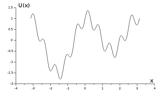
Figure 1: A double-well potential with additional small local minima.

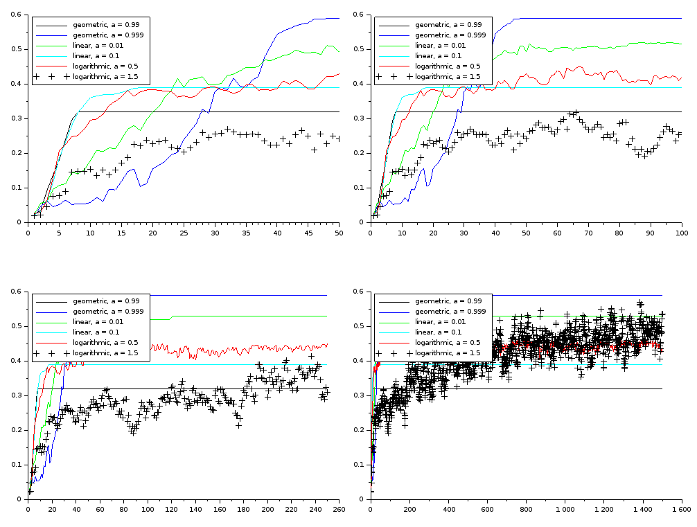
Figure 2: An approximation of $t\mapsto\mathbb{P}\left(U(X_{t})\leqslant\min U+0.25\right)$ for different time schedules. The four graphs are the same, except for the time window which is expanded. On the x-axis, each point represent in fact 100 steps of the Euler scheme. The line represented with crosses is the only case that satisfies the condition of Theorem 1.

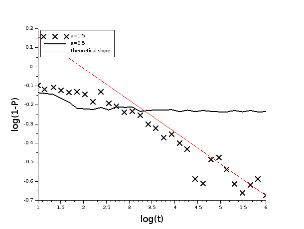
Figure 3: A $\log_{10}$-scale representation of the approximation of $t\mapsto 1-\mathbb{P}\left(U(X_{t})\leqslant\min U+0.25\right)$. The red line is the line with slope -1/6 which crosses the last point of the case $a=1.5$. Again, each graduation of the x-axis represents 100 Euler scheme steps.

Rather than of the process 9, we run an Euler-Maryuama discretization of the SDE

$$\left\{\begin{array}[]{rcl}\text{d}X_{t}&=&Y_{t}\text{d}t\\ &&\\ \text{d}Y_{t}&=&-\frac{\theta(\varepsilon_{t})}{\varepsilon_{t}}\nabla_{x}U(X_{t})\text{d}t-Y_{t}\text{d}t+\sqrt{2\theta(\varepsilon_{t})}\text{d}B_{t},\end{array}\right.$$

for which the instantaneous invariant measure is still the Gibbs law with temperature $\varepsilon$ and variance $\theta(\varepsilon)$ (the normalization of 9 has been chosen to lighten some computations, but the proofs of Theorem 1 can be straightforwardly adapted to this other one). Choosing $\theta(\varepsilon)=\varepsilon$, we compare two different geometric cooling schedule $\varepsilon_{k}=5a^{k}$ with $a=0.99$ and $0.999$, two linear ones $\varepsilon_{k}=5(1+ak)^{-1}$ with $a=0.1$ and $a=0.01$, and two logarithmic ones $\varepsilon_{k}^{-1}=1/5+\ln(1+k)/(aE_{*})$ with $a=0.5$ and $a=1.5$ (so that the initial temperature is 5 for all of them). In each case, 100 independent replicas of the process are run and we approximate the probability of success $\mathbb{P}\left(U(X_{t})\leqslant\min U+\delta\right)$ by the proportion of replicas for which $U(X_{t})\leqslant\min U+\delta$, or more precisely by the mean of this proportion in 100 successive steps. We chose $\delta=0.25$ so that the set $\{U\leqslant\min U+\delta\}$ is an interval which contains no other minimum than the global one.

The result is represented in Figure 2. Sooner or later, at some point, all the fast cooling schedule (geometric and linear) freeze, each replica being stuck in a given local minima, so that the proportion of them which are in the correct one stops to evolve after some time. After 12 000 steps of the Euler scheme, only the logarithmic cases still show some variation. But at that time, the probability to be in the right well, in those cases, is around 0.3 and 0.4. It grows with time, but very slowly.

Figure 3 represent, in a $\log_{10}$-scale, the approximation of $t\mapsto\mathbb{P}\left(U(X_{t})>\min U+0.25\right)$ for both logarithmic schedules. After $10^{6}$ iterations, the case $a=0.5$ stabilizes around the probability 0.4 of success. According to Theorem 1, in the case $a=1.5$, the probability of failure should decay at least as $t^{-1/6}$, and Figure 3 suggests that this is indeed the right order of magnitude. After $10^{8}$ Euler steps, the probability of success is about 0.8. Interpolating along the theoretical slope, it would take around $10^{10}$ Euler steps to reach a probability of success of 0.9.

2 Sketch of the proof

Some notations and the structure of the proof of Theorem 1 are given here at a formal level. It will be checked in the rest of the paper that the objects introduced here are well-defined and that the arguments can be made rigorous.

2.1 Hypocoercivity in the homogeneous case

Consider an homogeneous Markov process $(Z_{t})_{t\geq 0}$ on a Polish space $E$. Let $m_{t}$ be the law of $(Z_{t})$ and let $(P_{t})_{t\geq 0}$ and $L$ be, respectively, the associated semi-group and infinitesimal generator, defined on a suitable set $\mathcal{D}$ of non negative test functions $f$ on $E$ by

$$P_{t}f(z) = \mathbb{E}\left(f(Z_{t})\ |\ Z_{0}=z\right)$$

$$Lf = \underset{t\rightarrow 0}{\lim}\frac{P_{t}f-f}{t}.$$

Suppose that the process admits a unique invariant measure $\mu\in\mathcal{P}(E)$, where $\mathcal{P}(E)$ is the set of probability measures on $E$. Furthermore, suppose that $m_{0}$ and $P_{t}$ are such that $m_{t}\ll\mu$ for all $t\geq 0$. Then, $h_{t}=\frac{\text{d}m_{t}}{\text{d}\mu}$ is a weak solution of

$$\partial_{t}h_{t} = L^{*}h_{t},$$

where $L^{*}$ is the dual in $L^{2}(\mu)$ of $L$, defined by $\int f(Lg)\text{d}\mu=\int(L^{*}f)g\text{d}\mu$ for $f,g\in\mathcal{D}$.

For $\nu\in\mathcal{P}(E)$ and $f\in\mathcal{D}$ with $\int f\text{d}\nu=1$, we define the relative entropy $\text{Ent}_{\nu}(f)$ and the Fisher information $I_{\nu}(f)$ by

$$\text{Ent}_{\nu}(f) = \int f\ln f\text{d}\nu,$$

$$I_{\nu}(f) = \int\frac{|\nabla f|^{2}}{f}\text{d}\nu.$$

We say that $\nu$ satisfies a log-Sobolev inequality with constant $\lambda$ if $\text{Ent}_{\nu}(f)\leqslant\lambda I_{\nu}(f)$ for all $f\in\mathcal{D}$. In the classical case of the overdamped Langevin diffusion (the SDE (5) with a constant temperature $T$), the exponentially fast convergence of the entropy toward zero (which quantifies the convergence of the law of the process toward its equilibrium) is a direct consequence of the log-Sobolev inequality for $\mu$ and of the Gronwall Lemma, since in that case

$$\partial_{t}\left(\text{Ent}_{\mu}\left(e^{tL^{*}}f\right)\right) = -I_{\mu}\left(e^{tL^{*}}f\right).$$

In the kinetic Langevin case, however, the entropy dissipation is not equal to the full Fisher information, but to a partial one, which may vanish even out of equilibrium. In particular, the entropy doesn’t decrease at constant rate. The solution proposed in [26] is to introduce a distorted entropy

$$H_{\mu}(f) = \int\frac{|\nabla_{x}f+\nabla_{y}f|^{2}}{f}\text{d}\mu+\gamma\text{Ent}_{\mu}(f),$$

for some $\gamma>0$, whose dissipation along the semi-group will be larger than the Fisher information.

In fact, more generally, we could consider different quantities than those (and, for instance, work with the $L^{2}$-norm as in [8]). The main point is that what plays the role of the entropy, the Fisher Information, the distorted entropy and the distorted entropy dissipation,

$$K_{\mu}\left(f\right) := \left(\frac{\text{d}}{\text{d}t}\right)_{|t=0}\left(H_{\mu}\left(e^{tL^{*}}f\right)\right),$$

should be defined such that, for some positive $C,\rho,\lambda$,

$$H_{\mu}(f) \leq C\left(\text{Ent}_{\mu}(f)+I_{\nu}(f)\right),$$

$$K_{\mu}(f) \leq -\rho I_{\mu}(f),$$

$$\text{Ent}_{\mu}(f) \leq \lambda I_{\mu}(f).$$

That way,

$$\partial_{t}\left(H_{\mu}(e^{tL^{*}}f)\right)\leq-\frac{\rho}{(1+\lambda)C}H_{\mu}(e^{tL^{*}}f),$$

and Gronwall’s Lemma yields the exponentially fast decay of $H_{\mu}$, hence of the entropy.

Now, if $\mu$ is the Gibbs law at temperature $\varepsilon>0$ of some potential with several minima, it is known [17] that the optimal constant $\lambda$ in the log-Sobolev inequality scales as $\exp(E_{*}/\varepsilon)$, up to some sub-exponential factors. If we were to prove that the dependence of $\rho$ and $C$ with respect to $\varepsilon$ is sub-exponential, then the leading term of the rate of convergence of $H_{\mu}$ would be $\lambda^{-1}$, which is exactly the rate of convergence in the overdamped Langevin case.

2.2 The non-homogeneous case

As a second step, we consider a non-constant temperature. More precisely, let $(\varepsilon_{t})_{t\geq 0}$ be a non-increasing positive cooling schedule. For $\varepsilon>0$, let $L_{\varepsilon}$ and $\mu_{\varepsilon}$ be the generator and invariant measure of a process at fixed temperature $\varepsilon$. We call $L_{\varepsilon_{t}}$ and $\mu_{\varepsilon_{t}}$ the instantaneous generator and invariant measure of the inhomogeneous process. Under suitable regularity assumptions, there exists an inhomogeneous Markov process $(Z_{t})_{t\geq 0}$ such that the semi-group $(P_{s,t})_{0\leq s\leq t}$ defined by

$$P_{s,t}f(z)=\mathbb{E}\left(f(Z_{t})\ |\ Z_{s}=z\right)$$

satisfies $\partial_{t}P_{s,t}f=P_{s,t}L_{\varepsilon_{t}}f$ for all $s>0$ and suitable test functions $f\in\mathcal{D}$. We write $L_{\varepsilon}^{*}$ the dual of $L_{\varepsilon}$ in $L^{2}(\mu_{\varepsilon})$. Let $m_{t}=\mathcal{L}(Z_{t})$, and suppose that $m_{0}$ is such that $m_{t}\ll\mu_{\varepsilon_{t}}$ for all $t\geq 0$, so that

$$\partial_{t}\left(m_{t}\right) = \left(L_{\varepsilon_{t}}^{*}\left(\frac{\text{d}m_{t}}{\text{d}\mu_{\varepsilon_{t}}}\right)\right)\mu_{\varepsilon_{t}}.$$ (11)

In other words, writing $h_{t}=\frac{\text{d}m_{t}}{\text{d}\mu_{\varepsilon_{t}}}$ and assuming $\frac{\mu^{\prime}_{\varepsilon_{t}}}{\mu_{\varepsilon_{t}}}=\underset{s\downarrow 0}{\lim}\frac{1}{s}\left(\frac{\text{d}\mu_{\varepsilon_{t+s}}}{\text{d}\mu_{\varepsilon_{t}}}-1\right)$ exists and is finite,

$$\partial_{t}\left(h_{t}\right) = L_{\varepsilon_{t}}^{*}\left(h_{t}\right)-h_{t}\frac{\mu^{\prime}_{\varepsilon_{t}}}{\mu_{\varepsilon_{t}}}.$$ (12)

Denoting $H_{t}=H_{\mu_{\varepsilon_{t}}}(h_{t})$ and following the previous strategy, a new term appears in the derivative

$$\partial_{t}H_{t} = K_{t}+\varepsilon^{\prime}_{t}\widetilde{K}_{t},$$

where

$$K_{t}\ =\ K_{\mu_{\varepsilon_{t}}}(h_{t}) := \left(\frac{\text{d}}{\text{d}s}\right)_{|s=0}\left(H_{\mu_{\varepsilon_{t}}}\left(e^{sL_{t}^{*}}h_{t}\right)\right)$$

$$\widetilde{K}_{t}\ =\ \widetilde{K}_{\mu_{\varepsilon_{t}}}(h_{t}) := (\partial_{\eta})_{|_{\eta=0}}\left(H_{\mu_{{\varepsilon_{t}}+\eta}}\left(h_{t}\frac{\text{d}\mu_{{\varepsilon_{t}}}}{\text{d}\mu_{{\varepsilon_{t}}+\eta}}\right)\right).$$

In the kinetic Langevin case (as in the overdamped one, see [18]), we will be able to control $|\widetilde{K}_{t}|$ with some moments of the process, and to show that these moments’ growth with time is slower than any power of $t$. Furthermore $K_{t}\leqslant-\lambda_{t}H_{t}$, where $\lambda_{t}$ scales like $\exp(-E_{*}/\varepsilon_{t})$, and we will end up with an inequality of the form

$$\partial_{t}H_{t} \leqslant \left(a|\varepsilon_{t}^{\prime}|t^{\alpha}-bt^{-\alpha}e^{-\frac{E_{*}}{\varepsilon_{t}}}\right)H_{t}+c|\varepsilon_{t}^{\prime}|t^{\alpha},$$

where $\alpha$ may be chosen arbitrarily small, and $a,b,c>0$. The condition on $\varepsilon_{t}$ ensures that the negative term compensates the others and that $H_{t}$ goes to zero. By Pinsker’s Inequality, this means the total variation distance between $m_{t}$ the law of the process at time $t$ and its instantaneous equilibrium $\mu_{\varepsilon_{t}}$ goes to zero. Conclusion follows from the fact that, as $\varepsilon\rightarrow 0$, the mass of $\mu_{\varepsilon}$ concentrates on any neighbourhood of the global minima of $U$.

To make rigorous this sketch of proof, to sum up, here is what we have to do in the rest of the paper:

• Check that everything is well-defined, and that derivation under the integral sign is valid (we will need some truncation arguments).

• Bound $\widetilde{K}$ with some moments of the process, and obtain estimates on these moments.

• Check that the log-Sobolev inequality and the hypocoercive dissipation $K\leqslant-\rho I$ hold.

• Check that the dependences in $\varepsilon$ are sub-exponential everywhere, except in the log-Sobolev inequality.

2.3 Remarks

• For the kinetic Langevin dynamics, the hypocoercive dissipation has been proved by Villani in [26]. The link between $\widetilde{K}$ and some moment of the process appears in the classical annealing analysis of Holley and Stroock [14] and Miclo [18]. For the kinetic process, moment estimates have been proved at fixed temperature by Talay [24] via Lyapunov techniques.

• The crucial point is, in fact, the dependences with respect to $\varepsilon$. At fixed temperature, the distorted entropy method does not usually yield sharp estimates of the real convergence rate (apart, for now, from the Gaussian case [2, 19]). Nevertheless, as was already pointed out, since the log-Sobolev constant is exponentially small at low temperature [17], only the large deviation scale is relevant, and as long as the other computations stay at a sub-exponential level, they don’t need to be sharp.

• Given a Markov generator $L$ for which a measure $\mu$ is invariant, $(\mu,L)$ is said to satisfy a log-Sobolev inequality with constant $\lambda$ if, for all suitable $f$,

  $$\text{Ent}_{\mu}(f) \leqslant \lambda\int fL\left(\ln f\right)\text{d}\mu.$$

  We may call this a Markovian log-Sobolev inequality, in contrast with the classical (or metric) log-Sobolev inequality $\text{Ent}_{\mu}(f)\leqslant\lambda I_{\mu}$. The Markovian inequality depends on a law and some dynamics, while the classical one depends on a law and a gradient, hence a metric. In the classical overdamped langevin case, both coincide, but it is not the case in the kinetic Langevin one, where

  $$\int fL\left(\ln f\right)\text{d}\mu = \int\frac{|\nabla_{y}f|^{2}}{f}\text{d}\mu,$$

  for which a Markovian inequality cannot hold.

• The fact that the only relevant parameter (the log-Sobolev constant $\lambda$) is just defined from the measure $\mu$ and from the metric of $\mathbb{R}^{d}$, and does not depend on the generator, makes sense in view of our previous remark, according to which all reasonable continuous Markov processes devised to sample a Gibbs law should follow the same Arrhenius law, regardless of the local Markov dynamics.

3 Preliminary considerations

In this section, we consider the diffusion process $(X_{t},Y_{t})_{t\geq 0}$ on $\mathbb{R}^{2d}$ which solves the SDE (9). The associated generator at temperature $\varepsilon>0$ is

$$L_{\varepsilon} = y.\nabla_{x}-\left(\frac{y}{\theta(\varepsilon)}+\frac{\theta(\varepsilon)}{\varepsilon}\nabla_{x}U\right).\nabla_{y}+\Delta_{y},$$ (13)

and the corresponding invariant law is

$$\mu_{\varepsilon}\left(\text{d}x\text{d}y\right)=Z^{-1}e^{-\frac{U(x)}{\varepsilon}-\frac{y^{2}}{2\theta(\varepsilon)}}\text{d}x\text{d}y,$$

where $Z=\int e^{-\frac{U(x)}{\varepsilon}-\frac{y^{2}}{2\theta(\varepsilon)}}\text{d}x\text{d}y$ is the normalization constant. We write $\nabla_{x}\cdot$ and $\nabla_{y}\cdot$ the divergence operators with respect to the variables $x$ and $y$, so that in $L^{2}\left(\mu_{\varepsilon}\right)$, the dual operators of $\nabla_{x}$ and $\nabla_{y}$ are

$$\nabla_{x}^{*}=-\nabla_{x}\cdot+\frac{1}{\varepsilon}\nabla_{x}U\hskip 40.0pt\nabla_{y}^{*}=-\nabla_{y}\cdot+\frac{1}{\theta\left(\varepsilon\right)}y$$

and

$$L_{\varepsilon} = \theta(\varepsilon)\left(\nabla_{y}^{*}\nabla_{x}-\nabla_{x}^{*}\nabla_{y}\right)-\nabla_{y}^{*}\nabla_{y},$$

$$L^{*}_{\varepsilon} = \theta(\varepsilon)\left(\nabla_{x}^{*}\nabla_{y}-\nabla_{y}^{*}\nabla_{x}\right)-\nabla_{y}^{*}\nabla_{y}$$ (14)

$$= -y.\nabla_{x}+\left(\frac{\theta(\varepsilon)}{\varepsilon}\nabla_{x}U-\frac{y}{\theta(\varepsilon)}\right).\nabla_{y}+\Delta_{y}.$$

3.1 The Gibbs law at small temperature

As was noted in Section 2.2, in order to use hypocoercive arguments and prove that a distorted entropy converges to zero, the instantaneous equilibria $\left(\mu_{\varepsilon}\right)_{\varepsilon>0}$ should satisfy a so-called log-Sobolev inequality.

Under Assumption 1.i, this inequality is known. More precisely, let $\mathcal{C}^{\infty}_{+}(\mathbb{R}^{2d})$ be the set of smooth positive functions $f$ on $\mathbb{R}^{2d}$, and for $\nu\in\mathcal{P}\left(\mathbb{R}^{2d}\right)$, $f\in\mathcal{C}^{\infty}_{+}(\mathbb{R}^{2d})$ with $\int f\text{d}\nu=1$, let

$$\text{Ent}_{\nu}(f) = \int f\ln f\text{d}\nu,$$

$$I_{\nu}(f) = \int\frac{|\nabla f|^{2}}{f}\text{d}\nu$$

(which are always well-defined, possibly infinite). Recall we say that a function $\varepsilon\mapsto w(\varepsilon)$ is sub-exponential if $\varepsilon\ln w(\varepsilon)$ goes to 0 as $\varepsilon$ goes to 0

Proposition 2.

Under Assumption 1.i, there exists $E_{*}>0$, called the critical depth of $U$, and a sub-exponential $c$ such that, for all $f\in\mathcal{C}^{\infty}_{+}(\mathbb{R}^{2d})$ with $\int f\text{d}\mu_{\varepsilon}=1$,

$$\emph{Ent}_{\mu_{\varepsilon}}(f) \leq \max\left(\frac{\theta(\varepsilon)}{2},c(\varepsilon)e^{\frac{E_{*}}{\varepsilon}}\right)I_{\mu_{\varepsilon}}(f).$$ (15)

Proof.

Log-Sobolev inequalities tensorizes (cf [1]) and $\mu_{\varepsilon}$ is the Cartesian product of its $d$-dimensional marginals (in $x$ and $y$), so that it is sufficient to prove such an inequality for each marginal.

The second marginal is the image by the multiplication by $\sqrt{\theta(\varepsilon)}$ of the standard Gaussian law, which satisfies a log-Sobolev with constant $\frac{1}{2}$, so that it satisfies a log-Sobolev inequality with constant $\frac{\theta(\varepsilon)}{2}$.

As far as the first marginal is concerned, among several proofs, we refer to the recent work [17]. ∎

The description of $E_{*}$ is the following: it is the largest energy barrier the process has to overcome, starting from a non-global minimum of $U$, in order to reach a global one (see [17]).

According to Section 2.2 again, we also need to show that, as $\varepsilon$ goes to zero, the mass of $\mu_{\varepsilon}$ concentrates around the global minima of $U$:

Lemma 3.

For any $\delta,\alpha>0$, there exists $c>0$ such that, if $\left(\tilde{X},\tilde{Y}\right)$ is a r.v. with law $\mu_{\varepsilon}$, then,

$$\mathbb{P}\left(U\left(\tilde{X}\right)\ >\ \min U+\delta\right) \leqslant ce^{-\frac{\delta-\alpha}{\varepsilon}}.$$

Proof.

Denote by $vol$ the Lebesgue volume of a Borel set of $\mathbb{R}^{d}$, and, for $\beta>0$,

$$\mathcal{A}_{\beta} = \left\{x\in\mathbb{R}^{d},\ U(x)<\min U+\beta\right\}$$

$$\widetilde{\mathcal{A}_{\beta}} = \left\{x\in\mathbb{R}^{d},\ \beta<U(x)-\min U<\beta+|x|\right\}.$$

Since $U$ is quadratic at infinity, these sets are compact for any $\beta>0$. Then, we simply bound

$$\frac{\int\mathbb{1}_{x\notin\mathcal{A}_{\delta}}e^{-\frac{U(x)}{\varepsilon}}\text{d}x}{\int e^{-\frac{U(x)}{\varepsilon}}\text{d}x} \leqslant e^{-\frac{\delta-\alpha}{\varepsilon}}\frac{vol\left(\widetilde{\mathcal{A}_{\delta}}\right)+\int e^{-\frac{|x|}{\varepsilon}}\text{d}x}{vol\left(\mathcal{A}_{\alpha}\right)}\ \leqslant\ e^{-\frac{\delta-\alpha}{\varepsilon}}\frac{vol\left(\widetilde{\mathcal{A}_{\delta}}\right)+\int e^{-|x|}\text{d}x}{vol\left(\mathcal{A}_{\alpha}\right)}$$

for $\varepsilon<1$ (the bound is clear for $\varepsilon\geqslant 1$, since a probability is less than 1). ∎

Note that, rather than the crude bound $\int e^{-\frac{1}{\varepsilon}(U-\min U)}\geqslant e^{-\frac{\alpha}{\varepsilon}}vol(A_{\alpha})$, a Laplace method would give a bound of the right order, $\varepsilon^{-\frac{1}{2}}e^{-\frac{\delta}{\varepsilon}}$, instead of $e^{-\frac{\delta-\alpha}{\varepsilon}}$.

3.2 Existence and regularity for the density of the process

As a first step to make rigorous the computations announced in Section 2.2, we show in this section that the density of the process (9) is nice.

Proposition 4.

Under Assumptions 1, the process $(X,Y)$ is well-defined for all time, and the second moment $\mathbb{E}\left(|X_{t}|^{2}+|Y_{t}|^{2}\right)$ is finite for all $t>0$. Moreover, $m_{t}=\mathcal{L}aw(X_{t},Y_{t})$ admits a smooth density in $\mathcal{C}^{\infty}_{+}(\mathbb{R}^{2d})$ (still denoted by $m_{t}$) with respect to the Lebesgue measure.

Proof.

The s.d.e (9) admits a solution at least up to the (random) time the process explode to infinity. Consider the homogeneous Markov process $Z_{t}=(X_{t},Y_{t},t)_{t\geq 0}$, with generator $\mathcal{A}=L_{\varepsilon_{t}}+\partial_{t}$, and the Hamiltonian

$$G(x,y,t)=\frac{U(x)-\min U}{\varepsilon_{t}}+\frac{|y|^{2}}{2\theta(\varepsilon_{t})}+1.$$

Then, for all $s\leq t$,

$$\mathcal{A}G(x,y,s) = \frac{2-|y|^{2}}{2\theta(\varepsilon_{s})}-\varepsilon_{s}^{\prime}\left(\frac{U(x)-\min U}{(\varepsilon_{s})^{2}}+\theta^{\prime}(\varepsilon_{s})\frac{|y|^{2}}{2\theta^{2}(\varepsilon_{t})}\right)$$

$$\leq CG(x,y,s),$$

where $C$ depends on the uniform bounds on $[0,t]$ of $\varepsilon$, $\theta$ and their derivatives. Let $\tau_{N}=\inf\{s>0,\ G(Z_{s})>N\}$, so that by Itô’s formula,

$$\mathbb{E}\left(e^{-Ct\wedge\tau_{N}}G(Z_{t\wedge\tau_{N}})\right) \leq \mathbb{E}\left(G(Z_{0})\right)$$ (16)

$$\Rightarrow\hskip 20.0pt\mathbb{P}\left(\tau_{N}<t\right)\hskip 10.0pt\leq\hskip 10.0pt\frac{\mathbb{E}\left(G(Z_{t\wedge\tau_{N}})\right)}{N}\hskip 10.0pt\leq\hskip 10.0pt\frac{e^{Ct}\mathbb{E}\left(G(Z_{0})\right)}{N}\hskip 10.0pt\underset{N\rightarrow\infty}{\longrightarrow}0.$$

Hence, the process is non-explosive and, applying the monotone convergence Theorem in (16), we get $\mathbb{E}(G(Z_{t}))<\infty$ for all $t$, which implies $\mathbb{E}\left(|X_{t}|^{2}+|Y_{t}|^{2}\right)<\infty$.

The law of the process is a weak solution of the Kolmogorov forward equation (11), but from [25], since the Hörmander bracket condition is fulfilled, this equation admits a unique strong solution which is $\mathcal{C}^{\infty}$. ∎

In particular, $h_{t}=\frac{\text{d}m_{t}}{\text{d}\mu_{\varepsilon_{t}}}$ is well-defined and smooth.

Proposition 5.

For all $t>0$, $m_{t}>0$. In particular $h_{t}$ is bounded below by a positive constant on any compact set.

Proof.

Following [11, Lemma 4.2], it is sufficient to prove that the deterministic system associated to the diffusion is approximatively controllable, meaning that for any $z_{0},z_{1}\in\mathbb{R}^{2d}$, for any $\eta>0$ and for any $T>0$, there exists a control $u\in\mathcal{C}([0,T],\mathbb{R}^{d})$ such that the solution $z(t)=\left(x(t),y(t)\right)$ of

$$\left\{\begin{array}[]{ccl}x^{\prime}(t)&=&y(t),\\ y^{\prime}(t)&=&F_{t}(z(t))+u(t),\\ z(0)&=&z_{0},\end{array}\right.$$

where $F_{t}(x,y)=\frac{\nabla_{x}U(x)}{\varepsilon_{t}}+\frac{y}{\theta(\varepsilon_{t})}$, satisfies $|z(T)-z_{1}|\leq\eta$. Let $z^{*}(t)$ be the uncontrolled motion, namely the solution of the equation with $u=0$, and

$$\mathcal{O}=\left\{sz^{*}(t)+(1-s)z_{1},\ t\in[0,T],\ s\in[0,1]\right\}.$$

Since $\mathcal{O}\times[0,T]$ is compact, $M=\max\left(\|\nabla_{z}F_{t}\|_{L^{\infty}(\mathcal{O}\times[0,T])},\max\{y,\ (x,y)\in\mathcal{O}\}\right)$ is finite. Let $\delta>0$ be small enough. We define $u$ as follow:

• for $s\in[0,\delta]$, $u(s)=\frac{1}{\delta}\left(-y_{0}+\frac{x_{1}-x_{0}}{T}\right)$,

• for $s\in[\delta+\delta^{2},T-\delta-\delta^{2}]$, $u(s)=-F_{s}\left((1-s)x_{0}+sx_{1},\frac{x_{1}-x_{0}}{T}\right)$,

• for $s\in[T-\delta,T]$, $u(s)=\frac{1}{\delta}\left(-\frac{x_{1}-x_{0}}{T}+y_{1}\right)$,

• for $s\in[\delta,\delta^{2}]$ and $[T-\delta-\delta^{2},T-\delta]$, $u$ is linear.

Thus, taking $\delta$ small enough with respect to $M$, $z(\delta)$ and $z(\delta+\delta^{2})$ are arbitrarily close to $\left(x_{0},\frac{x_{1}-x_{0}}{T}\right)$, so that $z(T-\delta-\delta^{2})$ and $z(T-\delta)$ are arbitrarily close to $\left(x_{1},\frac{x_{1}-x_{0}}{T}\right)$, and $z(T)$ is arbitrarily close to $z_{1}$. ∎

3.3 Moment estimates

The aim of this subsection is to prove the following:

Proposition 6.

Under Assumptions 1, for all $p\in\mathbb{N}$ and $\alpha>0$, there exists a constant $k$ such that

$$\mathbb{E}\left(\left(U(X_{t})+|Y_{t}|^{2}\right)^{p}\right)\leq k(1+t)^{\alpha}.$$

This result will enable us to control the term denoted as $\widetilde{K}_{t}$ in Section 2.2.

We follow the methods of Talay [24] (see also [27]) and Miclo [18], making sure the temperature is only involved in sub-exponential functions.

Lemma 7.

Let $\delta^{-1}(\varepsilon)=4\left(1+\frac{1}{\sqrt{a_{1}l}}\right)\left(1+\frac{\varepsilon}{2r\theta^{3}\left(\varepsilon\right)}\right)$, and

$$R_{\varepsilon}(x,y) = \frac{\theta\left(\varepsilon\right)}{\varepsilon}U(x)+\frac{|y|^{2}}{2}+\delta(\varepsilon)x.y.$$

Then, there exist constants $c,C,\rho,N>0$ such that

$$c\left(U(x)+|y|^{2}\right)-N\hskip 15.0pt\leq\hskip 15.0ptR_{\varepsilon}(x,y)\hskip 15.0pt\leq\hskip 15.0ptC\left(\frac{\theta(\varepsilon)}{\varepsilon}U(x)+|y|^{2}\right)+N,$$

and

$$L_{\varepsilon}\left(R_{\varepsilon}\right) \leq -\rho\varepsilon^{2}R_{\varepsilon}+N\frac{\theta(\varepsilon)}{\varepsilon}.$$

Proof.

Since $\frac{\theta\left(\varepsilon\right)}{\varepsilon}\geq l$, $U(x)\geq a_{1}|x^{2}|-M$ and $\delta(\varepsilon)\leq\frac{1}{4}\sqrt{a_{1}l}$, we get

$$\frac{l}{2}U(x)+\frac{|y|^{2}}{4}-lM\hskip 15.0pt\leq\hskip 15.0ptR_{\varepsilon}(x,y)\hskip 15.0pt\leq\hskip 15.0pt\left(\frac{\theta\left(\varepsilon\right)}{\varepsilon}+l\right)U(x)+|y|^{2}+lM.$$

Next, notice that

$$L_{\varepsilon}\left(\frac{U}{\varepsilon}+\frac{|y|^{2}}{2\theta\left(\varepsilon\right)}\right) = -\frac{|y|^{2}}{\theta(\varepsilon)}+d,$$

where $d$ is the dimension. On the other hand,

$$L_{\varepsilon}\left(x.y\right) = |y|^{2}-\frac{y.x}{\theta\left(\varepsilon\right)}-\frac{\theta\left(\varepsilon\right)}{\varepsilon}\nabla_{x}U(x).x$$

$$\leq \left(1+\frac{\varepsilon}{2r\theta^{3}\left(\varepsilon\right)}\right)|y|^{2}-\frac{\theta\left(\varepsilon\right)}{2\varepsilon}\left(2\nabla_{x}U(x).x-r|x|^{2}\right)$$

$$\leq \frac{1}{2}\delta^{-1}(\varepsilon)|y|^{2}-\frac{r\theta\left(\varepsilon\right)}{2a_{1}\varepsilon}\left(U(x)-M\left(1+\frac{a_{1}}{r}\right)\right).$$

Hence, for some constants $c_{i}>0$,

$$L_{\varepsilon}\left(R_{\varepsilon_{t}}\right)(x,y) \leq -\frac{1}{2}|y|^{2}-c_{1}\frac{\delta\left(\varepsilon\right)\theta\left(\varepsilon\right)}{\varepsilon}U(x)+c_{2}\frac{\delta\left(\varepsilon\right)\theta\left(\varepsilon\right)}{\varepsilon}+d\theta\left(\varepsilon\right)$$

$$\leq -\delta\left(\varepsilon\right)\left(c_{3}|y|^{2}+c_{4}\left(\frac{\theta(\varepsilon)}{\varepsilon}+l\right)U(x)\right)+c_{5}\frac{\theta(\varepsilon)}{\varepsilon}$$

$$\leq -c_{6}\delta\left(\varepsilon\right)R_{\varepsilon}(x,y)+c_{7}\frac{\theta(\varepsilon)}{\varepsilon}.$$

Finally, from $\theta(\varepsilon)\geq l\varepsilon$ and the fact that $\varepsilon$ is non-increasing,

$$\delta^{-1}(\varepsilon)\hskip 15.0pt\leq\hskip 15.0ptc_{8}+\frac{c_{9}}{\theta^{2}(\varepsilon)}\hskip 15.0pt\leq\hskip 15.0pt\frac{c_{10}}{\varepsilon^{2}}.$$

∎

Lemma 8.

For all $p\in\mathbb{N}$, there is a sub-exponential $C_{p}(\varepsilon)$ such that

$$\partial_{\varepsilon}\left(R_{\varepsilon}^{p}\right) \leq C_{p}\left(\varepsilon\right)\left(R_{\varepsilon}^{p}+1\right).$$

Proof.

It is straightforward from the fact $\theta,\ \delta,\ \partial_{\varepsilon}\theta$ and $\partial_{\varepsilon}\delta$ are sub-exponential functions, since the product and sum of sub-exponential functions are still sub-exponential. ∎

Lemma 9.

For all $p\in\mathbb{N}$ and $\alpha>0$ there is a constant $\widetilde{C}_{p,\alpha}$ such that

$$\mathbb{E}\left[\left(R_{\varepsilon_{t}}(X_{t},Y_{t})\right)^{p}\right] \leq \widetilde{C}_{p,\alpha}(1+t)^{1+\alpha}.$$

Proof.

We prove this by induction. For $p=0$, the result is trivial. Let $p\geq 1$ and suppose that the result holds for all $q<p$. We write $n_{t,p}=\mathbb{E}\left[\left(R_{\varepsilon_{t}}(X_{t},Y_{t})\right)^{p}\right]$ the $p^{th}$ (distorted) moment at time $t$. Thanks to Lemma 8,

$$\partial_{t}\left(n_{t,p}\right) = \varepsilon_{t}^{\prime}\left.\partial_{\varepsilon}\right|_{\varepsilon=\varepsilon_{t}}\left(\mathbb{E}\left[\left(R_{\varepsilon}(X_{t},Y_{t})\right)^{p}\right]\right)+\partial_{s}|_{s=0}\left(\mathbb{E}\left[\left(R_{\varepsilon_{t}}(X_{t+s},Y_{t+s})\right)^{p}\right]\right)$$

$$\leq |\varepsilon_{t}^{\prime}|C_{p}\left(\varepsilon_{t}\right)\left(n_{t,p}+1\right)+\mathbb{E}\left[\left(L_{t}(R_{\varepsilon_{t}})^{p}\right)(X_{t},Y_{t})\right].$$

Since $L_{\varepsilon}$ is a second-order derivation operator, for any $\psi\in\mathcal{C}^{\infty}\left(\mathbb{R}\right)$, $L_{\varepsilon}\left(\psi(f)\right)=\psi^{\prime}(f)L_{\varepsilon}f+\psi^{\prime\prime}(f)\Gamma_{\varepsilon}(f)$ where $\Gamma_{\varepsilon}=\frac{1}{2}L_{\varepsilon}f^{2}-fL_{\varepsilon}f$ is the classical carré du champ operator. In the case of the kinetic Langevin process, $\Gamma_{\varepsilon}(f)=|\nabla_{y}f|^{2}$. On the other hand, for some $b_{i}>0$,

$$|\nabla_{y}R_{\varepsilon_{t}}|^{2} = |y+\delta(\varepsilon_{t})x|^{2}$$

$$\leq b_{1}R_{\varepsilon_{t}}+b_{2}.$$

Hence, from Lemma 7, using that $az^{p-1}+bz^{p-2}\leq(a+b)\left(z^{p-1}+1\right)$ for $p\geq 2$ and $z\geq 0$,

$$L_{\varepsilon_{t}}\left(R_{\varepsilon_{t}}^{p}\right) \leq pR_{\varepsilon_{t}}^{p-1}L_{\varepsilon_{t}}R_{\varepsilon_{t}}+p(p-1)(b_{1}+b_{2})\left(R_{\varepsilon_{t}}^{p-1}+1\right)$$

$$\leq -\rho p\varepsilon_{t}^{2}R_{\varepsilon_{t}}^{p}+b_{3}\frac{\theta\left({\varepsilon_{t}}\right)}{\varepsilon_{t}}\left(R_{\varepsilon_{t}}^{p-1}+1\right).$$

Thus,

$$\partial_{t}\left(n_{t,p}\right) \leq \left(|\varepsilon_{t}^{\prime}|C_{p}(\varepsilon_{t})-\rho p\varepsilon_{t}^{2}\right)n_{t,p}+b_{3}\frac{\theta\left({\varepsilon_{t}}\right)}{\varepsilon_{t}}(n_{t,p-1}+1)+|\varepsilon_{t}^{\prime}|C_{p}(\varepsilon_{t}).$$

Let $\alpha>0$. Since $\varepsilon_{t}\geq\frac{E}{A+\ln(1+t)}$, we get $C_{p}(\varepsilon_{t})=\underset{t\rightarrow\infty}{o}\left(t^{\beta}\right)$ for all $\beta>0$, and the same goes for $\frac{\theta(\varepsilon_{t})}{\varepsilon_{t}}$. By induction, and since $|\varepsilon_{t}^{\prime}|\leq\frac{b_{4}}{t}$,

$$\partial_{t}\left(n_{t,p}\right) \leq -b_{5}\varepsilon_{t}^{2}n_{t,p}+b_{6}\widetilde{C}_{p-1,\frac{\alpha}{4}}(1+t)^{1+\frac{\alpha}{2}}$$

$$\Rightarrow\hskip 20.0pt\partial_{t}\left(n_{t,p}e^{b_{5}\int_{0}^{t}\varepsilon^{2}_{s}\text{d}s}\right) \leq b_{7}(1+t)^{1+\frac{\alpha}{2}}e^{b_{5}\int_{0}^{t}\varepsilon^{2}_{s}\text{d}s}$$

$$\Rightarrow\hskip 88.0ptn_{t,p} \leq n_{0,p}+b_{7}(1+t)^{1+\frac{\alpha}{2}}\int_{0}^{t}e^{-b_{5}\int_{s}^{t}\varepsilon^{2}_{u}\text{d}u}\text{d}s$$

$$\leq n_{0,p}+b_{7}(1+t)^{1+\frac{\alpha}{2}}\int_{0}^{t}e^{-b_{5}\varepsilon^{2}_{t}(t-s)}\text{d}s$$

$$\leq n_{0,p}+\frac{b_{7}(1+t)^{1+\frac{\alpha}{2}}}{b_{5}\varepsilon^{2}_{t}}$$

$$\leq b_{8}(1+t)^{1+\alpha}.$$

∎

of Proposition 6.

From Lemma 7 and 9 and Jensen’s Inequality, there exist some $a_{1},a_{2}>0$ such that, for any $r\geq 1$,

$$\mathbb{E}\left(\left(U(X_{t})+|Y_{t}|^{2}\right)^{p}\right) \leq a_{1}+a_{2}\mathbb{E}\left(R^{p}_{\varepsilon_{t}}(X_{t},Y_{t})\right)$$

$$\leq a_{1}+a_{2}\left(\mathbb{E}\left(R^{pr}_{\varepsilon_{t}}(X_{t},Y_{t})\right)\right)^{\frac{1}{r}}$$

$$\leq a_{1}+a_{2}\widetilde{C}_{1,pr}(1+t)^{\frac{2}{r}},$$

which concludes since $r$ is arbitrarily large. ∎

4 Gamma calculus

In this section, we are interested, in a formal and general framework, in quantities of the form

$$\Gamma_{L,\Phi}(h)=\frac{1}{2}\left(L\Phi(h)-D_{h}\Phi(h).Lh\right),$$

where $L$ is a Markov operator, $h$ is a non negative function from $\mathbb{R}^{d}$ to $\mathbb{R}$ which belongs to some functional space $\mathcal{D}$, and $\Phi:\mathcal{D}\rightarrow\mathbb{R}$ is differentiable, with differential operator $D_{h}\Phi$. Such quantities naturally appear for the following reason: if $L$ admits an invariant measure $\mu$, then $\int L(g)\text{d}\mu=0$ for all suitable $g$, so that, writing $h_{t}=e^{tL}h$,

$$\partial_{t}\left(\int\Phi(h_{t})\text{d}\mu\right)=-\int\left(L\Phi(h_{t})-D_{h}\Phi(h_{t}).Lh_{t}\right)\text{d}\mu.$$

In particular, if $\Gamma_{L,\Phi}(h)\geq c\Phi(h)$ for all $h\in\mathcal{D}$ for some $c>0$ then, by the Gronwall’s Lemma,

$$\int\Phi(h_{t})\text{d}\mu\leq e^{-2ct}\int\Phi(h_{0})\text{d}\mu.$$

There is also a point-wise analogous to this computation: if for $s\in[0,t],$

$$\psi(s)=e^{sL}\left(\Phi(h_{t-s})\right),$$

then

$$\psi^{\prime}(s)=e^{sL}\left(L\Phi(h_{t-s})-D_{h}\Phi(h_{t-s}).Lh_{t-s}\right).$$

If $\Gamma_{L,\Phi}(h)\geq c\Phi(h)$, this yields

$$\Phi(h_{t})\leq e^{-2ct}e^{tL}\Phi(h_{0}).$$

Integrating with respect to $\mu$ brings back to $\int\Phi(h_{t})\text{d}\mu\leq e^{-2ct}\int\Phi(h_{0})\text{d}\mu$.

The Gamma calculus is thus a convenient way to retrieve some known computations related to hypocoercivity, in particular the derivation along a semi-group of the distorted entropy, which we will need in Section 5. We refer to [5, 1, 3] for an overview of classical Gamma calculus. The latter does not deal with hypoelliptic diffusions, so that we need to expand it in some sense, which is the aim of this section. This will give a new insight on the hypocoercive arguments of Villani [26], as has also been proposed by Baudoin in [4]. Our motivation is to control in a nice way the dependence with respect to the temperature of the estimates we obtain.

Note that, since the first submission of the present work, a more comprehensive presentation of the generalized Gamma presented below has been written in [19]. In particular, more general motivations are given, and the novelties with respect to both classical Gamma calculus and existing hypocoercivity results are discussed. This is not the core of the present paper, and thus, we won’t go into these details, and only present the computations which will prove useful in Section 5.

In the remainder of this section, we suppose the space $\mathcal{D}$ is such that everything is well-defined.

4.1 Quadratic $\Phi$’s

First, we consider the case where $\Phi(h)=|Ah|^{2}$ where $A=(A_{1},\dots,A_{k})$ is a linear operator from $\mathcal{D}$ to $\mathcal{D}^{k}$. In particular, if $A=I_{d}$, we retrieve the carré du champ operator which is simply denoted by $\Gamma$:

$$\Gamma(h)\ =\ \Gamma_{L,(.)^{2}}(h)\ =\ \frac{1}{2}L(h^{2})-hLh.$$

Another classical example would be $\Phi(h)=|\nabla h|^{2}$. For a general quadratic $\Phi$,

$$\Gamma_{L,\Phi}(h)\ =\ \frac{1}{2}L|Ah|^{2}-(Ah).A(Lh),$$

which directly yields the following:

Lemma 10.

If $\Phi(h)=|Ah|^{2}$, then

$$\Gamma_{L,\Phi}(h) = \Gamma(Ah)+(Ah)[L,A]h$$

where for two operator $C$ and $D$, $[C,D]=CD-DC$ and, by convention, we write $\Gamma(Ah)=\sum_{i=1}^{k}\Gamma(A_{i}h)$ and $[L,A]=\left([L,A_{1}],\dots,[L,A_{k}]\right)$.

In particular, since $\Gamma$ is always non-negative, $\Gamma_{L,\Phi}(h)\geq(Ah)[L,A]h$.

Example 1: consider the case of a diffusion process with a constant diffusion matrix $B$, namely

$$Lh(z)\ =\ b(z).\nabla h(z)+\nabla\cdot\left(B\nabla h(z)\right),$$

where $\nabla\cdot$ is the divergence operator. Given a constant matrix $M$, set $\Phi(h)=|M\nabla h|^{2}$. Then, $\Gamma(h)=\nabla h.B\nabla h$ and

$$\Gamma_{L,\Phi}(h) \geqslant (M\nabla h).[L,M\nabla]h$$

$$= -(M\nabla h).MJ_{b}\nabla h,$$

where $J_{b}$ is the Jacobian matrix of $b$. Now, suppose that there exists an invertible matrix $M$ for which $-MJ_{b}(z)M^{-1}$ is bounded below uniformly in $z$ as a quadratic form, meaning that

$$\forall x\in\mathbb{R}^{d},\hskip 20.0pt-x.MJ_{b}(z)M^{-1}x\ \geqslant\ \kappa|x|^{2}$$

for some $\kappa\in\mathbb{R}$ which does not depend on $z$. Note that this assumption holds in particular if $J_{b}$ is constant, in which case we retrieve the results of [2], or, when $B=M^{*}M$, if the process satisfies a classical Bakry-Emery curvature condition. In that case, writing $h_{t}=e^{tL}h$, we have

$$|M\nabla h_{t}|^{2}\ \leqslant\ e^{-2\kappa t}|M\nabla h_{0}|^{2},$$

and, in particular, $|\nabla h_{t}|^{2}\leq ce^{-2\kappa t}e^{tL}|\nabla h_{0}|^{2}$ for some $c>0$. Note that such a gradient/semi-group commutation is related to the contraction by $e^{tL}$ of the Wasserstein space $\mathcal{W}^{2}$ (see [15] for further considerations on this topic).

Example 2: consider the case of the kinetic Langevin operator

$$L = -y.\nabla_{x}+\left(\nabla_{x}U(x)-\frac{y}{\theta}\right).\nabla_{y}+\Delta_{y}.$$

Then, denoting by $\nabla^{2}_{x}U$ the Hessian matrix of $U$,

$$\ [L,\nabla_{x}]\ =\ -\nabla^{2}_{x}U\nabla_{y}, \ [L,\nabla_{y}]\ =\ \nabla_{x}+\frac{1}{\theta}\nabla_{y}.$$ (17)

If we assume that $\nabla^{2}_{x}U$ is bounded, then $\Gamma_{L,|\nabla.|^{2}}(h)\geq-\kappa|\nabla h|^{2}$ for $\kappa=\|\nabla_{x}^{2}U\|_{\infty}+1+\frac{1}{\theta}$, which would only yield, for $h_{t}=e^{tL}h_{0}$,

$$|\nabla h_{t}|^{2}\ \leqslant\ e^{2\kappa t}|\nabla h_{0}|^{2}.$$

Note that this is already more than what would give the Bakry-Emery criterion, since here the Bakry-Emery curvature is equal to $-\infty$.

Now, let $\Phi(h)=|(\nabla_{x}+\nabla_{y})h|^{2}=|M\nabla h|^{2}$, where $M$ is a $d\times(2d)$ matrix constituted of two Identity matrices side by side. In that case, from (17),

$$\Gamma_{L,\Phi}(h) \geqslant (\nabla_{x}+\nabla_{y})h.[L,\nabla_{x}+\nabla_{y}]h$$

$$= |\nabla_{x}h|^{2}+\left(\frac{1}{\theta}-\nabla_{x}^{2}U(x)\right)|\nabla_{y}h|^{2}+\left(1+\frac{1}{\theta}-\nabla_{x}^{2}U(x)\right)\nabla_{y}h.\nabla_{x}h$$

$$\geqslant |\nabla_{x}h|^{2}-\|\nabla_{x}^{2}U\|_{\infty}|\nabla_{y}h|^{2}-\left(1+\frac{1}{\theta}+\|\nabla_{x}^{2}U\|_{\infty}\right)\left|\nabla_{y}h.\nabla_{x}h\right|$$

$$\geqslant \frac{1}{2}|\nabla_{x}h|^{2}-2\left(\|\nabla_{x}^{2}U\|_{\infty}+1+\frac{1}{\theta}\right)^{2}|\nabla_{y}h|^{2}.$$

Writing $\beta=\frac{1}{2}+2\left(\|\nabla_{x}^{2}U\|_{\infty}+1+\frac{1}{\theta}\right)^{2}$ and $\Psi(h)=\Phi(h)+\beta h^{2}$, this reads

$$\Gamma_{L,\Psi}\ =\ \Gamma_{L,\Phi}(h)+\beta\Gamma(h)\ \geqslant\ \frac{1}{2}|\nabla h|^{2}.$$

Up to this point, we have not used the fact that $L$ admits an invariant measure $\mu$; in particular we have not used any information on $\mu$, and we have not split $L$ in its symmetric and anti-symmetric parts in $L^{2}(\mu)$, as it is usually done in the previous hypocoercive works (such as [26, Lemma 32]). The only assumption on $\mu$ we shall make for now is that it satisfies a Poincaré inequality, namely

$$\int\left(h-\int h\text{d}\mu\right)^{2}\text{d}\mu\leqslant\lambda\int|\nabla h|^{2}\text{d}\mu$$

for some $\lambda>0$. Then, replacing $h$ by $g=h-\int h\text{d}\mu$ in the above computation, we get

$$\int\Psi\left(g\right)\text{d}\mu\ \leqslant\ (2+\beta\lambda)\int|\nabla g|^{2}\text{d}\mu\ \leqslant\ 2(2+\beta\lambda)\int\Gamma_{L,\Psi}\left(g\right)\text{d}\mu\$$

and, by the Gronwall Lemma, since $\int h_{t}\text{d}\mu=\int h_{0}\text{d}\mu$ for all $t\geqslant 0$,

$$\int\Psi\left(h_{t}-\int h_{0}\text{d}\mu\right)\text{d}\mu\ \leqslant\ e^{-\frac{t}{2+\beta\lambda}}\int\Psi\left(h_{0}-\int h_{0}\text{d}\mu\right)\text{d}\mu.$$

4.2 Entropic $\Phi$’s

In this subsection, $L$ is a diffusion operator:

$$Lh\ =\ b\nabla h+\nabla\cdot\left(B\nabla h\right),$$

where $b$ is a vector field and $B$ is a symmetric positive matrix-valued function. This is equivalent to the fact that for any $\psi\in\mathcal{C}^{\infty}\left(\mathbb{R}\right)$,

$$L\left(\psi(h)\right) = \psi^{\prime}(h)Lh+\psi^{\prime\prime}(h)\Gamma(h),$$

$$L(gf) = gL(f)+fL(g)+2\Gamma(g,f),$$

where $\Gamma(f,g)$ stands for the symmetric bilinear operator associated by polarization to the quadratic operator $\Gamma$. We recall the following classical lemma:

Lemma 11.

If $\Phi(h)=h\ln h$ then

$$\Gamma_{L,\Phi}(h) = \frac{\Gamma(h)}{2h}.$$

Proof.

Let $\psi(x)=x\ln x$, so that $\psi^{\prime}(x)=1+\ln x$, $\psi^{\prime\prime}(x)=\frac{1}{x}$, and

$$2\Gamma_{L,\Phi}(h) = (1+\ln h)Lh+\frac{\Gamma(h)}{h}-(1+\ln h)Lh.$$

∎

Note that, since $\Gamma$ is the square of a first order differential operator, $\frac{\Gamma(h)}{h}=4\Gamma\left(\sqrt{h}\right)$. When the diffusion matrix of the generator is $I_{d}$ and $\mu$ is the invariant measure, $\int\Gamma(\sqrt{h})\text{d}\mu=\int|\nabla\sqrt{h}|^{2}\text{d}\mu$ and we retrieve the Fisher Information of $h$ with respect to $\mu$.

Let us consider, for a matrix-valued function $M\in\mathcal{C}^{2}\left(\mathbb{R}^{d},\mathcal{M}_{d}(\mathbb{R})\right)$,

$$\Phi_{M}(h) = \frac{|M\nabla h|^{2}}{h},$$

which may be called a Fisher Information-like term, even if $M$ is not invertible.

Lemma 12.

If $\Phi_{M}(h)=\frac{|M\nabla h|^{2}}{h}$, then

$$\Gamma_{L,\Phi_{M}}(h) \geq \frac{M\nabla h.[L,M\nabla]h}{h}.$$

Proof.

Making use of the diffusion property of $L$, we compute

$$\Gamma_{L,\Phi_{M}}(h) = \frac{1}{2}L\left(\frac{|M\nabla h|^{2}}{h}\right)-4M\nabla\sqrt{h}.M\nabla\left(\frac{Lh}{2\sqrt{h}}\right)$$

$$= \frac{1}{2}\frac{L\left(|M\nabla h|^{2}\right)}{h}+\frac{1}{2}|M\nabla h|^{2}L\left(\frac{1}{h}\right)+\Gamma\left(\frac{1}{h},|M\nabla h|^{2}\right)$$

$$-\frac{M\nabla h.M\nabla Lh}{h}-\frac{M\nabla h.M\nabla\left(h^{-\frac{1}{2}}\right)}{\sqrt{h}}Lh$$

$$= \frac{\Gamma_{L,|M\nabla.|^{2}}(h)}{h}+\Gamma\left(\frac{1}{h},|M\nabla h|^{2}\right)+|M\nabla h|^{2}\frac{\Gamma(h)}{h^{3}}.$$

From Lemma 10 and the fact that $\Gamma\left(\frac{1}{f},g^{2}\right)=-\frac{\Gamma(f,g^{2})}{f^{2}}=-\frac{2\Gamma(f,g)g}{f^{2}}$,

$$\Gamma_{L,\Phi_{M}}(h) = \frac{\Gamma\left(M\nabla h\right)+M\nabla h.[L,M\nabla]h}{h}-\frac{2\Gamma(h,M\nabla h).M\nabla h}{h^{2}}+|M\nabla h|^{2}\frac{\Gamma(h)}{h^{3}},$$

where by convention $\Gamma(h,M\nabla h)=\left(\Gamma\left(h,(M\nabla h)_{1}\right),\dots,\Gamma\left(h,(M\nabla h)_{d}\right)\right)$. As the diffusion matrix $B$ is symmetric and positive, $B=Q^{*}Q$ for some real matrix $Q$ and $\Gamma(f)=|Q\nabla f|^{2}$, which yields $|\Gamma(f,g)|\leq\sqrt{\Gamma(f)\Gamma(g)}$ and

$$-\frac{2\Gamma(h,M\nabla h).M\nabla h}{h^{2}} \geq -\frac{\Gamma\left(M\nabla h\right)}{h}-|M\nabla h|^{2}\frac{\Gamma(h)}{h^{3}}.$$

∎

Corollary 13.

Suppose

$$L = -y.\nabla_{x}+\left(\nabla_{x}U(x)-\frac{y}{\theta}\right).\nabla_{y}+\Delta_{y}$$

with $U$ such that $\|\nabla_{x}^{2}U\|_{\infty}<\infty$, and let

$$\beta = 1+2\left(\|\nabla_{x}^{2}U\|_{\infty}+1+\frac{1}{\theta}\right)^{2}$$

$$\Phi(h) = \frac{|(\nabla_{x}+\nabla_{y})h|^{2}}{h}+\beta h\ln h,$$

$$\Phi_{2}(h) = \frac{|\nabla h|^{2}}{h}.$$

Then

$$\Gamma_{L,\Phi} \geq \frac{1}{2}\Phi_{2}$$

$$\Gamma_{L,\Phi_{2}} \geq -\left(\|\nabla_{x}^{2}U\|_{\infty}+1+\frac{1}{\theta}\right)\Phi_{2}.$$

Proof.

All the computations have already been executed in Example 2 of Section 4.1. ∎

In Section 5, this result will be the core of the hypocoercivity dissipation introduced in Section 2. Note that we followed the ideas of [26, Lemma 32], but in a somehow simpler presentation, so that the dependences with respect to $U$ and $\theta$ is clear, and without using any information about the invariant measure.

5 Distorted entropy dissipation

We use here the notations of Section 3. In particular, $h_{t}=\frac{m_{t}}{\mu_{\varepsilon_{t}}}$, where $m_{t}$ is the law of the process (9). We now introduce the distorted entropy

$$H(t) = \int\frac{|\nabla_{x}h_{t}+\nabla_{y}h_{t}|^{2}}{h_{t}}\text{d}\mu_{\varepsilon_{t}}+\gamma\left(\varepsilon_{t}\right)\text{Ent}_{\mu_{\varepsilon_{t}}}(h_{t}),$$

where $\gamma(\varepsilon)=1+2\left(\frac{\theta(\varepsilon)}{\varepsilon}\|\nabla_{x}^{2}U\|_{\infty}+1+\frac{1}{\theta(\varepsilon)}\right)^{2}$. The aim of this section is to prove the following:

Proposition 14.

For all $t>0$, the Fisher information $I(t)=\int\frac{|\nabla h_{t}|^{2}}{h_{t}}\text{d}\mu_{\varepsilon_{t}}$ is finite, and $t\mapsto I(t)$ is locally bounded. Moreover, $H$ is absolutely continuous and there exists a sub-exponential function $\xi$ such that, for almost every $t\geq 0$,

$$H^{\prime}(t)\leq-I(t)+|\varepsilon_{t}^{\prime}|\xi(\varepsilon_{t})\left(H(t)+1+\mathbb{E}(X_{t}^{2}+Y_{t}^{2})\right).$$

Recall that, according to Section 2.2, such a differential inequality is the main technical argument in the proof of Theorem 1, since it will imply that $H(t)$, hence $\text{Ent}_{\mu_{\varepsilon_{t}}}(h_{t})$, goes to zero as $t$ goes to infinity.

5.1 Truncated differentiation

In the first instance, we will consider a truncated version of $H$ in order to differentiate under the integral sign. We write

$$\Phi_{0}(h) = h\ln h,$$

$$\Phi_{1}(h) = \frac{|(\nabla_{x}+\nabla_{y})h|^{2}}{h},$$

$$\Phi_{2}(h) = \frac{|\nabla h|^{2}}{h}.$$

These quantities are well-defined for $h\in\mathcal{D}=\{h\in\mathcal{C}^{\infty}(\mathbb{R}^{2d}),\ h>0\}$ and, for any smooth compactly-supported $\eta\in\mathcal{C}_{c}^{\infty}\left(\mathbb{R}^{2d}\right)$, so is $\int\eta\Phi_{i}(h)\text{d}\mu_{\varepsilon_{t}}$ for $i=0,1,2$. From Propositions 4 and 5, for all $t\geq 0$, $h_{t}\in\mathcal{D}$ and so does $m_{t}=h_{t}\mu_{\varepsilon_{t}}$.

Let $\mathcal{T}=\{\eta\in\mathcal{C}_{c}^{\infty}(\mathbb{R}^{2d}),0\leq\eta\leq 1\}$. We are interested in the truncated distorted entropy and the truncated Fisher information:

$$H_{\eta}(t) = \int\eta\left(\Phi_{1}(h_{t})+\gamma(\varepsilon_{t})\Phi_{0}(h_{t})\right)\text{d}\mu_{\varepsilon_{t}}$$

$$I_{\eta}(t) = \int\eta\Phi_{2}(h_{t})\text{d}\mu_{\varepsilon_{t}}.$$

In order to understand the time evolution of (the truncated versions of) $H$ and $I$, following the ideas of Section 2.2 (with the distinction between $K_{t}$ and $\widetilde{K}_{t}$), we will distinguish the roles of, on the one hand, the evolution of the temperature at fixed time (Lemma 15 below) and, on the other hand, the convergence to equilibrium at fixed temperature (Lemma 16 below).

Lemma 15.

There exists a sub-exponential function $\xi(\varepsilon)$ such that for all $\eta\in\mathcal{T}$ and for all $m\in\mathcal{D}$,

$$\partial_{\varepsilon}\left(\int\eta\Phi_{i}\left(\frac{m}{\mu_{\varepsilon}}\right)\text{d}\mu_{\varepsilon}\right) \leqslant \xi(\varepsilon)\left(\int\eta\Phi_{i}\left(\frac{m}{\mu_{\varepsilon}}\right)\text{d}\mu_{\varepsilon}+\int(1+x^{2}+y^{2})m(x,y)\text{d}x\text{d}y\right)$$

for $i=1,2$, and

$$\partial_{\varepsilon}\left(\gamma(\varepsilon)\int\eta\Phi_{0}\left(\frac{m}{\mu_{\varepsilon}}\right)\text{d}\mu_{\varepsilon}\right) \leqslant \xi(\varepsilon)\left(\gamma(\varepsilon)\int\eta\Phi_{0}\left(\frac{m}{\mu_{\varepsilon}}\right)\text{d}\mu_{\varepsilon}+\int(1+x^{2}+y^{2})m(x,y)\text{d}x\text{d}y\right).$$

Proof.

Note that $\Phi_{0}\left(\frac{m}{\mu_{\varepsilon}}\right)\mu_{\varepsilon}=\ln\left(\frac{m}{\mu_{\varepsilon}}\right)m$ and that $\Phi_{i}\left(\frac{m}{\mu_{\varepsilon}}\right)\mu_{\varepsilon}=\left|M_{i}\nabla\ln\left(\frac{m}{\mu_{\varepsilon}}\right)\right|^{2}m$ for $i=1,2$ for some matrices $M_{1},M_{2}$. Hence, we compute

$$\partial_{\varepsilon}\ln\mu_{\varepsilon}(x,y) = \frac{U(x)}{\varepsilon^{2}}+\frac{\partial_{\varepsilon}\theta\left(\varepsilon\right)|y|^{2}}{\theta^{2}(\varepsilon)}-\frac{\int\left(\frac{U(u)}{\varepsilon^{2}}+\frac{\partial_{\varepsilon}\theta\left(\varepsilon\right)|v|^{2}}{\theta^{2}(\varepsilon)}\right)e^{-\frac{U(u)}{\varepsilon}-\frac{|v|^{2}}{2\theta(\varepsilon)}}\text{d}u\text{d}v}{\int e^{-\frac{U(u)}{\varepsilon}-\frac{|v|^{2}}{2\theta(\varepsilon)}}\text{d}u\text{d}v}$$

$$= \frac{U(x)}{\varepsilon^{2}}+\frac{\partial_{\varepsilon}\theta\left(\varepsilon\right)|y|^{2}}{\theta^{2}(\varepsilon)}-\int\left(\frac{U(u)}{\varepsilon^{2}}+\frac{\partial_{\varepsilon}\theta\left(\varepsilon\right)|v|^{2}}{\theta^{2}(\varepsilon)}\right)\text{d}\mu_{\varepsilon}(\text{d}u,\text{d}v).$$

The moments of the family $(\mu_{\varepsilon})_{\varepsilon<1}$ are clearly bounded uniformly with respect to $\varepsilon$, so that there exists a sub-exponential $\xi_{1}$ such that

$$|\partial_{\varepsilon}\ln\mu_{\varepsilon}(x,y)|+|\nabla\partial_{\varepsilon}\ln\mu_{\varepsilon}(x,y)|^{2}\leqslant\xi_{1}(\varepsilon)(1+x^{2}+y^{2}).$$

It implies, using that $|\Phi_{0}(h)|=|\Phi_{0}(h)+\frac{1}{e}-\frac{1}{e}|\leq\Phi_{0}(h)+\frac{2}{e}$ (as $\frac{1}{e}=\underset{x\in\mathbb{R}}{\inf}\left(x\ln x\right)$), that

$$\partial_{\varepsilon}\left(\gamma(\varepsilon)\int\eta\Phi_{0}\left(\frac{m}{\mu_{\varepsilon}}\right)\mu_{\varepsilon}\right) = \int\eta\partial_{\varepsilon}\ln\mu_{\varepsilon}m+\gamma^{\prime}(\varepsilon)\int\eta\Phi_{0}\left(\frac{m}{\mu_{\varepsilon}}\right)\mu_{\varepsilon}$$

$$\leqslant \xi_{1}(\varepsilon)\int(1+x^{2}+y^{2})m(x,y)\text{d}x\text{d}y+|\gamma^{\prime}(\varepsilon)|\left(\int\eta\Phi_{0}\left(\frac{m}{\mu_{\varepsilon}}\right)\mu_{\varepsilon}+\frac{2}{e}\right)$$

and, for $i=1,2$,

$$\partial_{\varepsilon}\left(\int\eta\Phi_{i}\left(\frac{m}{\mu_{\varepsilon}}\right)\mu_{\varepsilon}\right) = -2\int M_{i}\nabla\ln\left(\frac{m}{\mu_{\varepsilon}}\right).M_{i}\nabla\partial_{\varepsilon}\ln\mu_{\varepsilon}\ \text{d}m$$

$$\leqslant \int\eta\Phi_{i}\left(\frac{m}{\mu_{\varepsilon}}\right)\mu_{\varepsilon}+2\xi_{1}(\varepsilon)\int(1+x^{2}+y^{2})m(x,y)\text{d}x\text{d}y.$$

Conclusion follows with $\xi=1+2\xi_{1}+\frac{|\gamma^{\prime}|}{\gamma}$. ∎

For the next Lemma, we use the notions and notations of Section 4.

Lemma 16.

Suppose that $\eta\in\mathcal{T}$ is such that $\left(2L_{\varepsilon}^{*}+L_{\varepsilon}\right)\eta\geqslant-c\eta$ for some $c>0$. Then, for all $h\in\mathcal{D}$,

$$\partial_{t}\left(\int\eta\Phi_{i}\left(e^{tL_{\varepsilon}^{*}}h\right)\text{d}\mu_{\varepsilon}\right) \leqslant c\left(\frac{1}{e}+\int\eta\Phi_{i}\left(e^{tL_{\varepsilon}^{*}}h\right)\text{d}\mu_{\varepsilon}\right)-2\int\eta\Gamma_{L_{\varepsilon}^{*},\Phi_{i}}\left(e^{tL_{\varepsilon}^{*}}h\right)\text{d}\mu_{\varepsilon}.$$

Proof.

In this proof, we write $h_{t}=e^{tL_{\varepsilon}^{*}}h$ (note that $\mathcal{D}$ is fixed by $e^{tL_{\varepsilon}^{*}}$ from Propositions 4 and 5 applied to the process with constant temperature schedule). Since the support of $\eta$ is compact, we can differentiate under the integral sign:

$$\partial_{t}\left(\int\eta\Phi_{i}\left(h_{t}\right)\text{d}\mu_{\varepsilon}\right) = \int\eta D\Phi_{i}\left(h_{t}\right).L_{\varepsilon}h_{t}\text{d}\mu_{\varepsilon}$$

$$= \int\eta D\Phi_{i}\left(h_{t}\right).L_{\varepsilon}^{*}h_{t}\text{d}\mu_{\varepsilon}-\int L_{\varepsilon}^{*}\left(\eta\Phi_{i}(h_{t})\right)\text{d}\mu_{\varepsilon}.$$

Since $L_{\varepsilon}^{*}$ is a diffusion operator,

$$L_{\varepsilon}^{*}\left(\eta\Phi_{i}(h_{t})\right)=\eta L_{\varepsilon}^{*}\Phi_{i}(h_{t})+\Phi_{i}(h_{t})L_{\varepsilon}^{*}\eta+2\Gamma_{\varepsilon}\left(\eta,\Phi_{i}(h_{t})\right),$$

and

$$\int\Gamma_{\varepsilon}(f,g)\text{d}\mu_{\varepsilon}=-\frac{1}{2}\int\left(fL_{\varepsilon}^{*}g+gL_{\varepsilon}^{*}f\right)\text{d}\mu_{\varepsilon}=-\frac{1}{2}\int f\left(L_{\varepsilon}^{*}+L_{\varepsilon}\right)g\text{d}\mu_{\varepsilon}.$$

Hence,

$$\partial_{t}\left(\int\eta\Phi_{i}\left(h_{t}\right)\text{d}\mu_{\varepsilon}\right) = -2\int\eta\Gamma_{L_{\varepsilon}^{*},\Phi_{i}}\left(h_{t}\right)\text{d}\mu_{\varepsilon}-\int\Phi_{i}(h_{t})\left(2L_{\varepsilon}^{*}+L_{\varepsilon}\right)(\eta)\text{d}\mu_{\varepsilon}$$

$$= -2\int\eta\Gamma_{L_{\varepsilon}^{*},\Phi_{i}}\left(h_{t}\right)\text{d}\mu_{\varepsilon}-\int\left(\Phi_{i}(h_{t})+\frac{1}{e}\right)\left(2L_{\varepsilon}^{*}+L_{\varepsilon}\right)(\eta)\text{d}\mu_{\varepsilon}.$$

The constant $\frac{1}{e}$ is added in order to ensure $\Phi_{i}(h)+\frac{1}{e}\geq 0$ for all $i=0,1,2$. We conclude with

$$\int\eta\text{d}\mu_{\varepsilon}\leqslant\int\text{d}\mu_{\varepsilon}=1.$$

∎

5.2 Construction of the truncation

We now describe a particular choice of $\eta\in\mathcal{T}$ which satisfies the assumption of Lemma 16.

Let $\kappa>0$ and

$$l(v)=\left\{\begin{array}[]{cll}1&&\text{if }v\leq-\frac{\pi}{\kappa},\\ \frac{-\kappa v-\sin(\kappa v)}{2\pi}+\frac{1}{2}&&\text{if }v\in\left[-\frac{\pi}{\kappa},\frac{\pi}{\kappa}\right],\\ 0&&\text{if }v\geq\frac{\pi}{\kappa}.\end{array}\right.$$

Then $l\in\mathcal{C}^{2}(\mathbb{R})$ is a non-increasing non-negative function with

$$l^{\prime\prime}(v)=\frac{\kappa^{2}}{2\pi}\sin(\kappa v)\mathbb{1}_{v\in\left[-\frac{\pi}{\kappa},\frac{\pi}{\kappa}\right]}\geq-\frac{\kappa^{2}}{2\pi}\mathbb{1}_{v\in\left[-\frac{\pi}{\kappa},0\right]}\geq-\frac{\kappa^{2}}{4\pi}l(v).$$

Let $\eta(x,y)=l\left(V(x,y)-p\right)$ for $p\in\mathbb{N}$, with $V$ to be chosen later in order to satisfy the following conditions:

• $V$ goes to $+\infty$ at $\infty$ (the level sets of $V$ are compact),

• $V$ is Lipschitz,

• $V$ is a Lyapunov function for $L_{\varepsilon_{t}}+2L_{\varepsilon_{t}}^{*}$, in the sense $\left(L_{\varepsilon_{t}}+2L_{\varepsilon_{t}}^{*}\right)V\leqslant 0$ outside a compact.

In the first instance, suppose that we have constructed such a function $V$. Let $\tilde{L}_{t}=2L_{\varepsilon_{t}}^{*}+L_{\varepsilon_{t}}$, and let $p$ be large enough so that the compact $\{\tilde{L}_{t}V\geq 0\}$ is included in $\{V\leq p-\frac{\pi}{\kappa}\}$. On $\{V\leq p-\frac{\pi}{\kappa}\}$, $\eta=1$ and thus $\tilde{L}_{t}\eta=0$. On $\{V\geq p-\frac{\pi}{\kappa}\}$, $\tilde{L}_{t}V\leq 0$ and thus

$$\tilde{L}_{t}\eta = l^{\prime}(V-p)\tilde{L}_{t}V+l^{\prime\prime}(V-p)\Gamma_{\tilde{L}_{t},(.)^{2}}(V)$$

$$\geqslant 3l^{\prime\prime}(V-p)|\nabla_{y}V|^{2}$$

$$\geqslant -\frac{3\kappa^{2}}{4\pi}\|\nabla_{y}V\|^{2}_{\infty}\eta.$$

Hence, in order to apply Lemma 16, it only remains to find a Lyapunov function $V$. The problem is that it has to be a Lyapunov function for $\tilde{L}_{t}$ uniformly in $t$, and it is not clear whether such a function exists. To solve this problem, we will work on small intervals of time.

Let $T>0$. In the following, we will call $\omega_{i}$, $i\in\mathbb{N}$, several constants that depend on $T$ but not on $t\in[0,T]$. Since $t\mapsto\varepsilon_{t}$ and $t\mapsto\theta(\varepsilon_{t})$ are locally Lipschitz functions, and from Assumption i, there exists $\omega_{1}>0$ such that for all $t,s\in[0,T]$,

$$|\left(\tilde{L}_{t}-\tilde{L}_{s}\right)f(x,y)|\leqslant\omega_{1}(1+|x|+|y|)|\nabla_{y}f|(x,y)|t-s|.$$

Let $R_{\varepsilon}$ be such as defined in Lemma 7. Then it is easy to see that there exist $\omega_{i}$, $i=2,3,4$, such that for all $t\in[0,T]$,

$$\tilde{L}_{t}R_{\varepsilon_{t}}(x,y) \leqslant -\omega_{2}(1+|x|+|y|)^{2}+\omega_{3},$$

$$|\nabla_{y}R_{\varepsilon}(x,y)| \leqslant \omega_{4}(1+|x|+|y|),$$

and thus

$$\tilde{L}_{s}R_{\varepsilon_{t}}(x,y) \leqslant -\omega_{2}(1+|x|+|y|)^{2}+\omega_{3}+\omega_{1}\omega_{4}(1+|x|+|y|)^{2}|t-s|.$$

In particular, if $|t-s|\leqslant\frac{\omega_{2}}{2\omega_{1}\omega_{4}}$, outside the compact set $\mathcal{K}=\{(1+|x|+|y|)^{2}\leq\frac{2\omega_{3}}{\omega_{2}}\}$,

$$L_{\varepsilon_{s}}R_{\varepsilon_{t}}(x,y) \leqslant 0.$$

Let $t_{0}=0<t_{1}<\dots<t_{N}=T$ be such that $|t_{n}-t_{n+1}|<\frac{\omega_{2}}{2\omega_{1}\omega_{4}}$, and let

$$V_{n}(x,y)=\sqrt{1+R_{\varepsilon_{t_{n}}}(x,y)-\underset{\mathbb{R}^{2}}{\min}R_{\varepsilon_{t_{n}}}}.$$

Then $V_{n}$ is a Lipschitz function and if $t\in[t_{n},t_{n+1}]$, outside $\mathcal{K}$,

$$\tilde{L}_{t}V_{n} = \frac{\tilde{L}_{t}R_{\varepsilon_{t_{n}}}}{2V_{n}}-\frac{\Gamma_{\tilde{L}_{t},(.)^{2}}\left(R_{\varepsilon_{t_{n}}}\right)}{2V_{n}^{3}}$$

$$\leq 0.$$

When $n$ and $\kappa$ are fixed, there exists $p_{0}$ such that $\mathcal{K}\subset\{V_{n}\leq p_{0}-\frac{\pi}{\kappa}\}$.

We are now ready to define our truncation:

$$\eta_{\kappa,p,n}=l(V_{n}-p)$$

(recall that $\kappa$ intervenes in the definition of $l$). In this section, we have proved the following:

Lemma 17.

For all $n\in\llbracket 0,N-1\rrbracket$, $\kappa>0$, $t\in[t_{n},t_{n+1}]$ and $p\geq p_{0}$, we have

$$\tilde{L}_{t}\eta_{\kappa,p,n}\geqslant-\frac{3\kappa^{2}}{4\pi}\|\nabla_{y}V_{n}\|^{2}\eta_{\kappa,p,n}.$$

5.3 End of the proof of Proposition 14

Bringing together Lemma 15,16 and 17 and the computations of Section 4, we get:

Lemma 18.

There exist $\omega_{5},\omega_{6}$ (depending only on $T$) such that for all $n\in\llbracket 0,N-1\rrbracket$, $\kappa>0$, $t\in[t_{n},t_{n+1}]$ and $p\geq p_{0}$, writing $\eta=\eta_{\kappa,p,n}$,

$$\partial_{t}I_{\eta}(t) \leq \omega_{5}\left(I_{\eta}(t)+1\right)$$

$$\partial_{t}H_{\eta}(t) \leq \omega_{6}\kappa^{2}\left(\frac{1}{e}+H_{\eta}(t)\right)-I_{\eta}(t)+|\varepsilon_{t}^{\prime}|\xi(\varepsilon_{t})\left(H_{\eta}(t)+1+\mathbb{E}(X_{t}^{2}+Y_{t}^{2})\right).$$

Proof.

Let $\omega_{6}=\frac{3}{4\pi}\underset{0\leq n\leq N-1}{\max}\|\nabla_{y}V_{n}\|_{\infty}$ and $\omega_{7}=\underset{\varepsilon_{0}\geq\varepsilon\geq\varepsilon_{T}}{\max}\left(\frac{\theta\left(\varepsilon\right)}{\varepsilon}\|\nabla_{x}U\|_{\infty}+1+\frac{1}{\theta\theta\left(\varepsilon\right)}\right)$. From Corollary 13, for all $t\in[0,T]$,

$$\Gamma_{L^{*}_{\varepsilon_{t}},\Phi_{2}}\geq-\omega_{7}\Phi_{2}.$$

Hence, from Lemma 15,16, and 17, by taking $\kappa=1$, $n\in\llbracket 0,N-1\rrbracket$ and $p\geq p_{0}$, we get

$$\partial_{t}I_{\eta}(t) \leq \omega_{6}\left(\frac{1}{e}+I_{\eta}(t)\right)+2\omega_{7}I_{\eta}(t)+|\varepsilon_{t}^{\prime}|\xi(\varepsilon_{t})\left(I_{\eta}(t)+1+\mathbb{E}\left(X_{t}^{2}+Y_{t}^{2}\right)\right)$$

$$\leq \omega_{5}(I_{\eta}(t)+1)$$

for some $\omega_{5}$ (the moments are uniformly bounded on $[0,T]$ according to Proposition 6). The case of $H_{\eta}$ is exactly the same. ∎

of Proposition 14.

From Lemma 18, for all $n\in\llbracket 0,N-1\rrbracket$, for all $t\in[t_{n},t_{n+1}]$, and for all $p$ large enough,

$$I_{\eta_{1,p,n}}(t)+1 \leq e^{\omega_{5}(t-t_{n})}\left(I_{\eta_{1,p,n}}(t_{n})+1\right).$$

When $p$ goes to infinity, the Fatou Lemma yields $I(t)+1\leq e^{\omega_{5}(t-t_{n})}\left(I(t_{n})+1\right)$, and thus, $I(t)+1\leq e^{\omega_{5}t}\left(I(0)+1\right)$ for all $t\in[0,T]$. Finally, $I(0)<\infty$ since

$$|\nabla\sqrt{h_{0}}|^{2}\mu_{\varepsilon_{0}} = \left|\nabla\sqrt{h_{0}\mu_{\varepsilon_{0}}}-\sqrt{h_{0}}\nabla\sqrt{\mu_{\varepsilon_{0}}}\right|^{2}$$

$$\leq 2|\nabla\sqrt{m_{0}}|^{2}+2h_{0}|\nabla\sqrt{\mu_{\varepsilon_{0}}}|^{2}$$

$$\leq 2|\nabla\sqrt{m_{0}}|^{2}+\frac{1}{2}m_{0}|\nabla\ln\mu_{\varepsilon_{0}}|^{2},$$

which is integrable according to Assumption 1.iv.

Note that, by the log-Sobolev inequality (15), this implies that $t\mapsto H_{t}$ is also finite and locally bounded. Integrating the second part of Lemma 18 between times $s,t\in[t_{n},t_{n+1}]$ yields, for $p$ large enough and writing $\eta=\eta_{\kappa,p,n},$

$$H_{\eta}(t)-H_{\eta}(s) \leq \int_{s}^{t}\omega_{6}\kappa^{2}\left(\frac{1}{e}+H_{\eta}(u)\right)-I_{\eta}(u)+|\varepsilon_{u}^{\prime}|\xi(\varepsilon_{u})\left(H_{\eta}(u)+\mathbb{E}(X_{u}^{2}+Y_{u}^{2})\right)\text{d}u.$$

Again, we let $p$ go to infinity and use the Fatou Lemma to get

$$H(t)-H(s) \leq \int_{s}^{t}\omega_{6}\kappa^{2}\left(\frac{1}{e}+H(u)\right)-I(u)+|\varepsilon_{u}^{\prime}|\xi(\varepsilon_{u})\left(H(u)+\mathbb{E}(X_{t}^{u}+Y_{t}^{u})\right)\text{d}u.$$

Then, let $\kappa$ go to 0: the result does not depend on $n$, or even on $T$ any more, and thus it is true for any $t,s>0$. ∎

6 Conclusion

We keep here the notations of the previous section. As announced in Section 2.2, the differential inequality satisfied by the distorted entropy implies it goes to zero:

Lemma 19.

Under Assumption 1, for any $\alpha>0$, there exists $B>0$ such that

$$H(t) \leqslant B\left(\frac{1}{t}\right)^{1-\frac{E_{*}}{E}-\alpha}.$$

Proof.

The log-Sobolev inequality (15) implies $I(t)\geq\xi_{2}(\varepsilon_{t})e^{-\frac{E_{*}}{\varepsilon_{t}}}H(t)$ for all $t>0$, where $\xi_{2}$ is a sub-exponential function, so that Proposition 14 becomes

$$H^{\prime}(t)\leq-\xi_{2}(\varepsilon_{t})e^{-\frac{E_{*}}{\varepsilon_{t}}}H(t)+|\varepsilon_{t}^{\prime}|\xi(\varepsilon_{t})\left(H(t)+1+\mathbb{E}(X_{t}^{2}+Y_{t}^{2})\right).$$

Since $\xi$ is sub-exponential and $\varepsilon_{t}\ln t$ is bounded below by a positive constant for $t$ large enough (from the slow cooling assumption), then $\forall\alpha>0$,

$$t^{-\alpha}\xi\left(\varepsilon_{t}\right)\ =\ e^{-\ln t\left(\alpha-\frac{1}{\varepsilon_{t}\ln t}\left(\varepsilon_{t}\ln\xi\left(\varepsilon_{t}\right)\right)\right)}\ \underset{t\rightarrow+\infty}{\longrightarrow}\ 0,$$

and similarly for $\xi_{2}$. Moreover, for $t$ large enough, $|\varepsilon_{t}^{\prime}|\leq\frac{\varepsilon_{0}^{2}}{Dt}$ which, together with Proposition 6, means that, for any $\alpha>0$,

$$\beta(t)\ :=\ |\varepsilon^{\prime}_{t}|\xi(\varepsilon_{t})\left(1+\mathbb{E}(X_{t}^{2}+Y_{t}^{2})\right)\ =\ \underset{t\rightarrow+\infty}{o}(t^{-1+\alpha}).$$

Similarly, for any $\alpha>0$, there exists $c>0$ such that, for $t$ large enough,

$$b(t)\ :=\ \xi_{2}(\varepsilon_{t})e^{-\frac{E_{*}}{\varepsilon_{t}}}\ \geqslant\ c\left(\frac{1}{t}\right)^{\frac{E_{*}}{E}+\alpha},$$

and $\beta=o(b)$ as $t\rightarrow\infty$. Hence, since $H>0$, $(b-\beta)H\geqslant\frac{1}{2}bH$ for large times, which means there exist $t_{0},c_{1},c_{2}$ such that for all $t\geqslant t_{0}$,

$$H^{\prime}(t)\ \leqslant\ -c_{1}\left(\frac{1}{t}\right)^{\frac{E_{*}}{E}+\alpha}H(t)+c_{2}\left(\frac{1}{t}\right)^{1-\alpha}.$$

As proved in [18, Lemma 6], this implies that $H$ goes to zero. For the sake of completeness, and to precise a speed of convergence toward zero, we recall here this short argument: if $\alpha\leqslant\frac{1}{2}\left(1-\frac{E_{*}}{E}\right)$, for $t_{0}$ large enough and for all $t\geq s\geq t_{0}$,

$$\partial_{s}\left(H(s)-\frac{2c_{2}}{c_{1}}\left(\frac{1}{s}\right)^{1-\frac{E_{*}}{E}-2\alpha}\right) \leqslant -c_{1}\left(\frac{1}{s}\right)^{\frac{E_{*}}{E}+\alpha}\left(H(s)-\frac{2c_{2}}{c_{1}}\left(\frac{1}{s}\right)^{1-\frac{E_{*}}{E}-2\alpha}\right),$$

or in other words

$$\partial_{s}\left(\left(H(s)-\frac{2c_{2}}{c_{1}}\left(\frac{1}{s}\right)^{1-\frac{E_{*}}{E}-2\alpha}\right)e^{c_{1}\int_{t_{0}}^{s}\left(\frac{1}{u}\right)^{\frac{E_{*}}{E}+\alpha}\text{d}u}\right) \leqslant 0.$$

As a consequence,

$$H(t) \leq \frac{2c_{2}}{c_{1}}\left(\frac{1}{t}\right)^{1-\frac{E_{*}}{E}-2\alpha}+H(t_{0})e^{-\frac{c_{1}}{v}(t^{v}-t_{0}^{v})},$$

where $v=1-\frac{E_{*}}{E}-\alpha>0$, which concludes. ∎

We can now conclude the proof of our main result:

Proof of Theorem 1.

For all $t\geq 0$, let $(\tilde{X}_{t},\tilde{Y}_{t})$ be a random variable with law $\mu_{\varepsilon_{t}}$. Then for all $\delta>0$,

$$\mathbb{P}\left(U(X_{t})>\min U+\delta\right) \leqslant \mathbb{P}\left(U(\tilde{X}_{t})>\min U+\delta\right)+\|h_{t}-1\|_{L^{1}(\mu_{\varepsilon_{t}})}.$$

By Pinsker’s inequality,

$$\|h_{t}-1\|_{L^{1}(\mu_{\varepsilon_{t}})}\ \leqslant\ \sqrt{2\text{Ent}_{\mu_{\varepsilon_{t}}}(h_{t})}\leq\sqrt{2H(t)}.$$

From Lemmas 19 and 3, for all $\delta,\alpha>0$, there exists $c>0$ such that

$$\mathbb{P}\left(U(X_{t})>\min U+\delta\right) \leqslant c\left(\left(\frac{1}{t}\right)^{\frac{1-\frac{E_{*}}{E}-\alpha}{2}}+e^{-\frac{\delta-\alpha}{\varepsilon_{t}}}\right).$$

The rhs goes to zero as $t$ goes to infinity, and is of order $\left(\frac{1}{t}\right)^{\frac{\min\left(\delta,\frac{E-E_{*}}{2}\right)-\alpha}{E}}$ if $\partial_{t}\left(\frac{1}{\varepsilon_{t}}\right)=\frac{1}{Et}$ for $t$ large enough. ∎

Acknowledgments

The author would like to thank Laurent Miclo, who initiated this work, for numerous fruitful discussions. This work has been supported by ANR STAB.

References

• [1] C. Ané, S. Blachère, D. Chafaï, P Fougères, I. Gentil, F. Malrieu, C. Roberto, and G. Scheffer. Sur les inégalités de Sobolev logarithmiques. Panoramas et synthèses. Société mathématique de France, Paris, 2000.
• [2] A. Arnold and J. Erb. Sharp entropy decay for hypocoercive and non-symmetric Fokker-Planck equations with linear drift. ArXiv e-prints, September 2014.
• [3] D. Bakry, I. Gentil, and M. Ledoux. Analysis and geometry of Markov diffusion operators, volume 348 of Grundlehren der Mathematischen Wissenschaften [Fundamental Principles of Mathematical Sciences]. Springer, Cham, 2014.
• [4] F. Baudoin. Bakry-Emery meet Villani. ArXiv e-prints, August 2013.
• [5] F. Bolley and I. Gentil. Phi-entropy inequalities for diffusion semigroups. J. Math. Pures Appl. (9), 93(5):449–473, 2010.
• [6] O. Catoni. Rough large deviation estimates for simulated annealing: application to exponential schedules. Ann. Probab., 20(3):1109–1146, 1992.
• [7] T.-S. Chiang, C.-R. Hwang, and S.J. Sheu. Diffusion for global optimization in ${\mathbb{R}}^{n}$. SIAM J. Control Optim., 25(3):737–753, 1987.
• [8] J. Dolbeault, C. Mouhot, and C. Schmeiser. Hypocoercivity for kinetic equations with linear relaxation terms. C. R. Math. Acad. Sci. Paris, 347(9-10):511–516, 2009.
• [9] G. Fort, B. Jourdain, E. Kuhn, T. Lelièvre, and G. Stoltz. Efficiency of the Wang-Landau algorithm: a simple test case. Appl. Math. Res. Express. AMRX, (2):275–311, 2014.
• [10] S. Gadat and L. Miclo. Spectral decompositions and $\mathbb{L}^{2}$-operator norms of toy hypocoercive semi-groups. Kinet. Relat. Models, 6(2):317–372, 2013.
• [11] S. Gadat and F. Panloup. Long time behaviour and stationary regime of memory gradient diffusions. Ann. Inst. Henri Poincaré Probab. Stat., 50(2):564–601, 2014.
• [12] A. Guillin and P. Monmarché. Optimal linear drift for an hypoelliptic diffusion. Electronic Communication of Probability, 21, 2016.
• [13] R. A. Holley, S. Kusuoka, and D. W. Stroock. Asymptotics of the spectral gap with applications to the theory of simulated annealing. J. Funct. Anal., 83(2):333–347, 1989.
• [14] R. A. Holley and D. W. Stroock. Simulated annealing via Sobolev inequalities. Comm. Math. Phys., 115(4):553–569, 1988.
• [15] K. Kuwada. Duality on gradient estimates and Wasserstein controls. J. Funct. Anal., 258(11):3758–3774, 2010.
• [16] T. Lelièvre, M. Rousset, and G. Stoltz. Long-time convergence of an adaptive biasing force method. Nonlinearity, 21(6):1155–1181, 2008.
• [17] G. Menz and A. Schlichting. Poincaré and logarithmic Sobolev inequalities by decomposition of the energy landscape. Ann. Probab., 42(5):1809–1884, 2014.
• [18] L. Miclo. Recuit simulé sur $R^{n}$. Étude de l’évolution de l’énergie libre. Ann. Inst. H. Poincaré Probab. Statist., 28(2):235–266, 1992.
• [19] P. Monmarché. Generalized $\Gamma$ calculus and application to interacting particles on a graph. ArXiv e-prints, October 2015.
• [20] P. Monmarché. Piecewise deterministic simulated annealing. ALEA Lat. Am. J. Probab. Math. Stat., 13(1):357–398, 2016.
• [21] Virgile Robbe. Small eigenvalues of the low temperature linear relaxation boltzmann equation with a confining potential. Annales Henri Poincaré, 17(4):937–952, Apr 2016.
• [22] A. Scemama, T. Lelièvre, G. Stoltz, and M. Caffarel. An efficient sampling algorithm for variational monte carlo. Journal of Chemical Physics, 125, September 2006.
• [23] Y. Sun and A. Garcia. Interactive diffusions for global optimization. J. Optim. Theory Appl., 163(2):491–509, 2014.
• [24] D. Talay. Stochastic Hamiltonian systems: exponential convergence to the invariant measure, and discretization by the implicit Euler scheme. Markov Process. Related Fields, 8(2):163–198, 2002.
• [25] S. Taniguchi. Applications of Malliavin’s calculus to time-dependent systems of heat equations. Osaka J. Math., 22(2):307–320, 1985.
• [26] C. Villani. Hypocoercivity. Mem. Amer. Math. Soc., 202(950):iv+141, 2009.
• [27] L. Wu. Large and moderate deviations and exponential convergence for stochastic damping Hamiltonian systems. Stochastic Process. Appl., 91(2):205–238, 2001.
• [28] P-A Zitt. Annealing diffusions in a potential function with a slow growth. Stochastic Process. Appl., 118(1):76–119, 2008.