Improved Lower Bounds on the Ground-State Entropy of the Antiferromagnetic Potts Model

Abstract

We present generalized methods for calculating lower bounds on the ground-state entropy per site, $S_{0}$, or equivalently, the ground-state degeneracy per site, $W=e^{S_{0}/k_{B}}$, of the antiferromagnetic Potts model. We use these methods to derive improved lower bounds on $W$ for several lattices.

I Introduction

Nonzero ground-state entropy, $S_{0}\neq 0$, is an important phenomenon in statistical mechanics. An example of this is water ice, for which $S_{0}=0.82\pm 0.05$ cal/(K-mole), i.e., $S_{0}/R=0.41\pm 0.03$ i35 -berg07 . A model with $S_{0}\neq 0$ is the $q$-state Potts antiferromagnet (AF) on a lattice $\Lambda$ for sufficiently large $q$ wurev . This subject also has an interesting connection with graph theory, since the partition function of the $q$-state Potts antiferromagnet at temperature $T=0$ on a graph $G$ is

$$Z(G,q,T=0)_{PAF}=P(G,q)\ ,$$ (1)

where $P(G,q)$ is the chromatic polynomial of $G$, which is equal to the number of ways of coloring the vertices of $G$ with $q$ colors subject to the constraint that adjacent vertices must have different colors. Such a color assignment is called a proper vertex $q$-coloring of $G$. The minimum number of colors required for a proper vertex $q$-coloring of the graph $G$ is called the chromatic number of the graph, denoted $\chi(G)$. We will focus here on regular $N$-vertex lattice graphs $\Lambda_{N}$ and, in particular, on the thermodynamic limit $N\to\infty$ (with appropriate boundary conditions), which will be denoted simply as $\Lambda$. In this limit, the ground-state (i.e., zero-temperature) degeneracy per vertex (site) of the $q$-state Potts antiferromagnet on $\Lambda$ is given by

$$W(\Lambda,q)=\lim_{N\to\infty}P(\Lambda_{N},q)^{1/N}\ ,$$ (2)

and the associated ground-state entropy per site is given by $S_{0}(\Lambda,q)=k_{B}\,\ln W(\Lambda,q)$. It will be convenient to express our bounds on the ground-state entropy per site in terms of its exponent, $e^{S_{0}(\Lambda,q)/k_{B}}=W(\Lambda,q)$.

In ww ; w3 by S.-H. Tsai and one of us (RS), lower bounds on $W(\Lambda,q)$ were derived for the triangular ($tri$), honeycomb ($hc$), $(4\cdot 8^{2})$, and $sq_{d}$ lattices. Here an Archimedean lattice $\Lambda$ is defined as a uniform tiling of the plane with a set of regular polygons such that all vertices are equivalent. Our notation for an Archimedean lattice follows the standard mathematical format wn ; gsbook , namely $\Lambda=(\prod_{i}p_{i}^{a_{i}})$, where the product is over the regular polygons $p_{i}$ that are traversed in a circuit around a vertex and $a_{i}\geq 1$ refers to possible contiguous repetitions of a given type of polygon in such a traversal. The $sq_{d}$ lattice is a nonplanar lattice formed from the square lattice by adding edges (bonds) connecting the two sets of diagonal next-nearest-neighbor vertices in each square. In wn , Shrock and Tsai derived corresponding lower bounds on $W(\Lambda,q)$ for all Archimedean lattices $\Lambda$ and their planar duals, using a coloring compatibility matrix (CCM) method employed earlier by Biggs for the square ($sq$) lattice biggs77 , in combination with the Perron-Frobenius theorem pf and a theorem giving a lower bound on the maximal eigenvalue of a symmetric non-negative matrix london .

In this paper we introduce several generalizations of the method used in ww -biggs77 and apply these to derive improved lower bounds on $W(\Lambda,q)$ for several lattices $\Lambda$. Refs. biggs77 and ww ; w3 also used CCM methods to derive upper bounds on $W(\Lambda,q)$. However, it was shown in ww ; w3 that, while the upper bounds were moderately restrictive, the lower bounds were very close to the actual values of $W(\Lambda,q)$. Therefore, as in wn , we focus here on the lower bounds on $W(\Lambda,q)$.

This paper is organized as follows. In Section II we explain the basic coloring compatibility matrix method. In Section III we discuss our generalizations of this method. In Sections IV-VI we apply our generalized methods to derive new and more restrictive lower bounds on $W(\Lambda,q)$ for the square, triangular, and honeycomb lattices. In Sections VII and VIII we present corresponding results for two heteropolygonal Archimedean lattices, namely, the $(4\cdot 8^{2})$ and $(3\cdot 6\cdot 3\cdot 6)$ (i.e., kagomé) lattices. In Section IX we report results for the $sq_{d}$ lattice. In Section X we compare the large-$q$ Taylor series expansions of our lower bounds for the various lattices with the large-$q$ series expansions of the actual $W$ functions for these respective lattices. Our conclusions are given in Section XI. We list some results on $r$-partite lattices in Appendix A, the lower bounds on $W(\Lambda,q)$ for Archimedean lattices $\Lambda$ from ww -biggs77 in Appendix B, and some higher-degree algebraic equations that are used in the text in Appendix C.

II Basic Calculational Method

In this section we explain the basic calculational method used in ww -biggs77 to derive lower bounds on $W(\Lambda,q)$. In the next section we generalize this method in several ways. We consider a sequence of (regular) lattices of type $\Lambda$ of length $L_{x}=n$ vertices in the longitudinal direction and width $L_{y}=m$ vertices in the transverse direction. In the thermodynamic limit $n\to\infty$, $m\to\infty$ with the aspect ratio $m/n$ finite, the boundary conditions do not affect $W(\Lambda,q)$. It will be convenient to take periodic boundary conditions (PBCs) in both directions. If a lattice $\Lambda$ is $r$-partite, then $m$ and $n$ are chosen so as to maintain this property.

The construction of the coloring compatibility matrix $T$ begins by considering an $n$-vertex path ${\cal P}_{n}$ in the longitudinal direction on $\Lambda$. The number of proper vertex $q$-colorings of ${\cal P}_{n}$ is the chromatic polynomial $P({\cal P}_{n},q)$. Now focus on two adjacent parallel paths, ${\cal P}_{n}$ and ${\cal P}^{\prime}_{n}$. Define compatible proper $q$-colorings of the vertices of these adjacent paths as proper $q$-colorings such that no two adjacent vertices on ${\cal P}_{n}$ and ${\cal P}^{\prime}_{n}$ have the same color. One can then associate with this pair of adjacent paths an ${\cal N}\times{\cal N}$ dimensional symmetric matrix $T$, where ${\cal N}=P({\cal P}_{n},q)=P({\cal P}^{\prime}_{n},q)$, with entries $T_{{\cal P}_{n},{\cal P}^{\prime}_{n}}=T_{{\cal P}^{\prime}_{n},{\cal P}_{n}}=$ 1 or 0 if the proper $q$-colorings of ${\cal P}_{n}$ and ${\cal P}^{\prime}_{n}$ are or are not compatible, respectively. This matrix is thus defined in the space of allowed color configurations for these adjacent paths.

It follows that, for fixed $m$ and $n$,

$$P(\Lambda_{m\times n},q)={\rm Tr}(T^{m})\ .$$ (3)

For a given $n$, since $T$ is a nonnegative matrix, one can apply the Perron-Frobenius theorem pf to conclude that $T$ has a real positive maximal eigenvalue $\lambda_{max}$. Hence, for fixed $n$,

$$\lim_{m\to\infty}Tr(T^{m})^{\frac{1}{mn}}=(\lambda_{max})^{\frac{1}{n}}\ .$$ (4)

Therefore, taking the $n\to\infty$ limit,

$$W(\Lambda,q)=\lim_{n\to\infty}(\lambda_{max})^{\frac{1}{n}}\ .$$ (5)

Let us denote the column sum

$$\kappa_{j}(T)=\sum_{i=1}^{\cal N}T_{ij}\ ,$$ (6)

which is equal to the row sum,

$$\rho_{j}(T)=\sum_{i=1}^{\cal N}T_{ji}\ ,$$ (7)

(since $T^{T}=T$) and the sum of all entries of $T$ as

$$S(T)=\sum_{i,j=1}^{\cal N}T_{ij}\ .$$ (8)

Note that $S(T)/{\cal N}$ is the average row sum (equal to the average column sum).

For a general nonnegative ${\cal N}\times{\cal N}$ matrix $A$, pf , one has

$$\min\{\kappa_{j}(A)\}\leq\lambda_{max}(A)\leq\max\{\kappa_{j}(A)\}$$ (9)

and

$$\min\{\rho_{j}(A)\}\leq\lambda_{max}(A)\leq\max\{\rho_{j}(A)\}$$ (10)

for $j=1,...,{\cal N}$. Since $T^{T}=T$, these are equivalent here. One also has the following more restrictive one-parameter family of lower bounds depending on the parameter $k$, for a symmetric nonnegative matrix $T$ london :

$$\biggl{[}\frac{S(T^{k})}{\cal N}\biggr{]}^{1/k}\leq\lambda_{max}(T)\ .$$ (11)

Refs. ww -biggs77 derived lower and upper bounds on $W(\Lambda,q)$ using the $k=1$ special case of (11). We will denote a generic lower bound on $W(\Lambda,q)$ with the subscript $\ell$, as $W(\Lambda,q)_{\ell}$. We will distinguish specific lower bounds that we obtain with the additional subscripts $b$ and $k$, as explained below. The lower bounds obtained in ww -biggs77 were for $b=1$ and $k=1$. Refs. ww -wn studied how close the upper and lower bounds obtained on $W(\Lambda,q)$ were to the actual values of $W(\Lambda,q)$ for a number of lattices, where the latter were determined mainly from Monte Carlo calculations, augmented by large-$q$ series expansions together with a few exact results. It was found that for a given lattice $\Lambda$, as $q$ increases beyond the region of $\chi(\Lambda)$, the lower bounds rapidly approach very close to the actual value of $W(\Lambda,q)$.

We next introduce some notation that will be used below for reduced functions obtained from $W(\Lambda,q)$ which will be analyzed in the large-$q$ limit. This large-$q$ limit is the natural one to consider for chromatic polynomials, since the constraint in a proper $q$-coloring of the vertices of a graph, namely that no two adjacent vertices have the same color, becomes progressively less restrictive as the number of colors increases to large values. The chromatic polynomial of an arbitrary $N$-vertex graph $G$ is a polynomial of degree $N$, and consequently, $W(\Lambda,q)\sim q$ as $q\to\infty$. In order to deal with a finite quantity in the $q\to\infty$ limit, one therefore considers the reduced ($r$) function $W_{r}(\Lambda,q)=W(\Lambda,q)/q$. A variable equivalent to $1/q$ that is convenient to use for a large-$q$ series expansion of $W_{r}(\Lambda,q)$ is $y=1/(q-1)$. These large-$q$ (i.e., small-$y$) series expansions are normally given for the function

$$\overline{W}(\Lambda,y)=\frac{W_{r}(\Lambda,q)}{(1-q^{-1})^{\Delta_{\Lambda}/2}}=\frac{W(\Lambda,q)}{q(1-q^{-1})^{\Delta_{\Lambda}/2}}\ ,$$ (12)

where $\Delta_{\Lambda}$ is the lattice coordination number of the lattice $\Lambda$ (i.e., the degree of the vertices of $\Lambda$). In terms of the expansion variable $y$, these series thus have the form $\overline{W}(\Lambda,y)=1+\sum_{k=1}^{\infty}w_{\Lambda,k}y^{k}$. Analogously, for the expansion of our lower bound, we define the reduced lower bound function $\overline{W}(\Lambda,y)_{\ell}$ as

$$\overline{W}(\Lambda,y)_{\ell}=\frac{W(\Lambda,q)_{\ell}}{q(1-q^{-1})^{\Delta_{\Lambda}/2}}\ .$$ (13)

Before proceeding, we note a subtlety in the definition of $W(\Lambda,q)$. As pointed out in w , the formal eq. (2) is not, in general, adequate to define $W(\Lambda,q)$ because of a noncommutativity of limits

$$\lim_{N\to\infty}\lim_{q\to q_{s}}P(\Lambda_{N},q)^{1/N}\neq\lim_{q\to q_{s}}\lim_{N\to\infty}P(\Lambda_{N},q)^{1/N}$$ (14)

at certain special points $q_{s}$. We denote the definitions based on the first and second orders of limits in (14) as $W(\Lambda,q)_{D_{Nq}}$ and $W(\Lambda,q)_{D_{qN}}$, respectively. This noncommutativity can occur for $q<q_{c}(\Lambda)$, where $q_{c}(\Lambda)$ denotes the maximal (finite) real value of $q$ where $W(\Lambda,q)$ is nonanalytic w . These values include $q_{c}(sq)=3$, $q_{c}(tri)=4$, and the formal value $q_{c}(hc)=(3+\sqrt{5})/2=2.618...$ wurev ; w for the square, triangular, and honeycomb lattices. As explained in w , the underlying reason for the noncommutativity is that as $q$ decreases from large values, there is a change in the analytic expression for $W(\Lambda,q)$ as $q$ decreases through the value $q_{c}(\Lambda)$. We do not have to deal with this complication here because elementary results yield exact values of $W(sq,2)$, $W(hc,2)$, $W((4\cdot 8^{2}),2)$, and $W(tri,3)$ (see Eqs. (207) and (208)), namely

$$W(sq,2)=W(hc,2)=W((4\cdot 8^{2}),2)=1,\quad W(tri,3)=1\ .$$ (15)

Hence, our lower bounds are not needed at the respective values $q=2$ for the square, honeycomb, and $(4\cdot 8^{2})$ lattices or for $q=3$ on the triangular lattice, and we therefore focus on their application to $q\geq 3$ for $\Lambda=sq,\ hc,\ (4\cdot 8^{2})$ and to $q\geq 4$ for $\Lambda=tri$, and similarly for other lattices.

III Generalized Coloring Compatibility Matrix Method

III.1 Coloring Compatibility Matrix Joining Adjacent Strips of Width $b$

The lower bounds on $W(\Lambda,q)$ derived in ww -biggs77 for various lattices $\Lambda$ used Eq. (11) with $T$ being a coloring compatibility matrix joining adjacent paths and with $k=1$. Here we generalize this method in several ways. Our first generalization is to use a coloring compatibility matrix that joins adjacent strips of width $b\geq 2$ vertices, rather than adjacent one-dimensional ($b=1$) paths. For simplicity, we explain this for the square lattice; similar discussions apply for other lattices. We define the matrix $T$ to enumerate compatible colorings of a strip of transverse width $b$ vertices and an adjacent parallel strip of width $b$ and arbitrary length $L_{x}$ vertices, with cyclic boundary conditions. (Here, by cyclic boundary conditions for a given strip, we mean in the $x$, i.e., longitudinal, direction along this strip). The condition that these strips are adjacent is equivalent to the statement that they share a common set of edges. Thus, this CCM is an ${\cal N}\times{\cal N}$ matrix, where ${\cal N}$ is the chromatic polynomial for the cyclic strip of width $b$ vertices and arbitrary length $L_{x}$, with cyclic boundary conditions. For this CCM, the sum of elements $S(T)$ is equal to the chromatic polynomial of a strip of width $L_{y}=2b-1$ vertices and arbitrary length $L_{x}$ vertices with cyclic boundary conditions. These chromatic polynomials of lattice strips of a fixed width $L_{y}$ and arbitrarily great length $L_{x}$ with periodic boundary conditions in the longitudinal direction and free boundary conditions in the transverse direction have the form

$$P(\Lambda,L_{y}\times L_{x},cycl.,q)=\sum_{d=0}^{L_{y}}c^{(d)}\sum_{j=1}^{n_{P}(L_{y},d)}(\lambda_{sq,L_{y},d,j})^{L_{x}}$$ (16)

with

$$c^{(d)}=\sum_{j=0}^{d}(-1)^{j}\,{2d-j\choose j}\,q^{d-j}\ ,$$ (17)

where ${a\choose b}=a!/[b!(a-b)!]$ is the binomial coefficient. For a table of the $n_{P}(L_{y},d)$, see cf . Because of the limits (4) and (5), only the largest $\lambda_{\Lambda,L_{y},d,j}$ enters in the lower bound (11) in the thermodynamic limit. As specific studies such as wcy -k showed, the dominant $\lambda$ for the values of $q$ of relevance here is $\lambda_{\Lambda,L_{y},0,1}$.

Applying this generalization of the coloring compatibility matrix in combination with the $k=1$ case of (11), we derive the new lower bound for $b\geq 2$:

$$W(\Lambda,q)\geq W(\Lambda,q)_{\ell;b,1}\ ,$$ (18)

where

$$W(\Lambda,q)_{\ell;b,1}=\Bigg{[}\frac{\lambda_{\Lambda,2b-1,0,1}}{\lambda_{\Lambda,b,0,1}}\Bigg{]}^{\frac{1}{b-1}}\ .$$ (19)

The final subscript, 1, in $W(\Lambda,q)_{\ell;b,1}$ in (18) and (19) is the value of $k$.

The corresponding lower bound for $\overline{W}(\Lambda,y)$ is

$$\overline{W}(\Lambda,y)\geq\overline{W}(\Lambda,y)_{\ell;b,1}\ ,$$ (20)

where, in accordance with Eq. (12),

$$\overline{W}(\Lambda,y)_{\ell;b,1}=\frac{W(\Lambda,q)_{\ell;b,1}}{q(1-q^{-1})^{\Delta_{\Lambda}/2}}\ ,$$ (21)

with $\Delta_{\Lambda}$ being the coordination number of the lattice $\Lambda$, as before. The inequality (18) with (19) is actually an infinite family of lower bounds depending on the strip width $b=1,2,...$, and similarly with (20) and (21). This is one of our two major results, which we will proceed to apply to a number of different lattices. The special case $b=1$ was previously used in biggs77 and ww -wn to derive lower bounds which we denote here as $W(\Lambda,q)_{\ell;1,1}$ and correspondingly $\overline{W}(\Lambda,y)_{\ell;1,1}$. Our generalization in this subsection is to $b\geq 2$ with $k=1$.

III.2 Coloring Compatibility Matrix Acting $k$ Times Joining Paths of Width $b=1$

Our second generalization is to use a coloring compatibility matrix method that involves paths (i.e., one-dimensional strips, with $b=1$) on $\Lambda$ that are separated by $k$ edges, where $k\geq 2$, rather than the situation with $b=1$ and $k=1$ considered in ww -wn , where the paths were adjacent. This means using the coloring compatibility matrix $T$ defined as connecting adjacent paths, and having it operate $k$ times, with $k\geq 2$. Hence, ${\cal N}=P(C_{L_{x}},q)$ and $S(T^{k})$ is the chromatic polynomial of a strip of width $L_{y}=k+1$ vertices and arbitrary length $L_{x}$ vertices with cyclic boundary conditions. Again, only the dominant $\lambda_{\Lambda,L_{y},d,j}$ terms enter in (11) in the thermodynamic limit. Using this method in combination with (11), we derive the lower bound

$$W(\Lambda,q)\geq W(\Lambda,q)_{\ell;1,k}\ ,$$ (22)

where

$$W(\Lambda,q)_{\ell;1,k}=\Bigg{[}\frac{\lambda_{\Lambda,k+1,0,1}}{\lambda_{\Lambda,1,0,1}}\Bigg{]}^{\frac{1}{k}}\ .$$ (23)

In (22) and (23), the first subscript after $\ell;$ is $b=1$.

An important theorem extending the result (11) is that for a symmetric nonnegative matrix $T$ merikoski84 ,

$$\biggl{[}\frac{S(T^{k})}{\cal N}\biggr{]}^{1/k}\quad{\rm is\ an\ increasing\ function\ of}\ k\ .$$ (24)

It follows that, for the physical range of $q$ of relevance for our application to a lattice $\Lambda$,

$$W(\Lambda,q)_{\ell;1,k}\quad{\rm is\ an\ increasing\ function\ of}\ k\ .$$ (25)

The corresponding lower bound for $\overline{W}(\Lambda,y)$ is

$$\overline{W}(\Lambda,y)\geq\overline{W}(\Lambda,y)_{\ell;1,k}\ ,$$ (26)

where, in accordance with Eq. (12),

$$\overline{W}(\Lambda,y)_{\ell;1,k}=\frac{W(\Lambda,q)_{\ell;1,k}}{q(1-q^{-1})^{\Delta_{\Lambda}/2}}\ .$$ (27)

Again, the inequality (22) with (23) is actually a one-parameter family of lower bounds depending on the parameter $k=1,2,...$, and similarly with (26) and (27). This is the second of our major results. The special case $k=1$ (with $b=1$) was previously used in ww -biggs77 ; the generalization presented in this subsection is to $k\geq 2$ with $b=1$. We have also carried out further generalizations of lower bounds on $W(\Lambda,q)$ with both $b\geq 2$ and $k\geq 2$. These are more complicated and will be presented elsewhere.

III.3 Measures of Improvement of Bounds

For a lattice $\Lambda$ and a given $q$, we define the ratio of a lower bound $W(\Lambda,q)_{\ell;b,k}$ to the actual value of $W(\Lambda,q)$ as

$$R_{\Lambda,q;\ell;b,k}\equiv\frac{W(\Lambda,q)_{\ell;b,k}}{W(\Lambda,q)}\ .$$ (28)

This ratio is useful as a measure of how close a particular lower bound $W(\Lambda,q)_{\ell;b,k}$ is to the actual value of the ground-state degeneracy per vertex, $W(\Lambda,q)$. For most lattices and values of $q$, the value of $W(\Lambda,q)$ is not known exactly, but rather is determined for moderate values of $q$ by Monte Carlo simulations, as discussed in ww ; w3 and, for larger values of $q$, by large-$q$ series expansions kimenting . Special cases of $\Lambda$ and $q$ for which exact results are known will be noted below.

An important property of our new lower bounds is that, for a given lattice $\Lambda$, they are larger than and hence more restrictive than the bounds $W(\Lambda,q)_{\ell;1,1}$ derived in ww -biggs77 . Since the lower bounds $W(\Lambda,q)_{\ell;1,1}$ were very close to the actual values of $W(\Lambda,q)$ for all but the lowest values of $q$, our improved lower bounds are even closer to these actual values. For the same reason, our new lower bounds yield the greatest fractional improvement for low to moderate values of $q$ and are only slightly greater than $W(\Lambda,q)_{\ell;1,1}$ for larger values of $q$. This will be evident in our explicit results. For our present discussion, we take $T$ to be the matrix that acts $k$ times mapping a strip of width $b$ to an adjacent strip of width $b$ on $\Lambda$. Then the theorem (24) and its corollary (25) imply that, for fixed $b$, the ratio of our lower bound $W(\Lambda,q)_{\ell;b,k}$ to the actual value $W(\Lambda,q)$ is an increasing function of $k$, i.e.,

$$R_{\Lambda,q;\ell;b,k}\quad{\rm is\ an\ increasing\ function\ of}\ k\ .$$ (29)

That is, as $k$ increases, the lower bound $W(\Lambda,q)_{\ell;b,k}$ becomes more restrictive. From our analysis, we also find that for fixed $k=1$ and $b\geq 2$,

$$R_{\Lambda,q;\ell;b,1}\quad{\rm is\ an\ increasing\ function\ of}\ b\ .$$ (30)

For a given $\Lambda$ and $q$, it is also of interest to compare the various lower bounds with each other. For this purpose, we define the ratio

$$R_{\Lambda,q;(b,k)/(b^{\prime},k^{\prime})}\equiv\frac{W(\Lambda,q)_{\ell;b,k}}{W(\Lambda,q)_{\ell;b^{\prime},k^{\prime}}}\ .$$ (31)

By the same argument, theorem (24) and its corollary (25) imply that for a given lattice $\Lambda$, our new lower bounds $W(\Lambda,q)_{\ell;1,k}$ improve on the bound $W(\Lambda,q)_{\ell;1,1}$ derived in ww -biggs77 : $W(\Lambda,q)_{\ell;1,k}\geq W(\Lambda,q)_{\ell;1,1}$, i.e.,

$$R_{\Lambda,q;(1,k)/(1,1)}\geq 1\quad{\rm for}\ k\geq 2\ .$$ (32)

We observe also that

$$R_{\Lambda,q;(b,1)/(1,1)}\geq 1\quad{\rm for}\ b\geq 2\ .$$ (33)

As will be evident from our explicit results, for the range of $q$ that we consider, these inequalities are realized as strict inequalities. As noted above, since the latter lower bounds $W(\Lambda,q)_{\ell;1,1}$ are very close to the actual values of $W(\Lambda,q)$, even for $q$ only moderately above $\chi(\Lambda)$, as shown in Table I of ww and Tables I-III of w3 , our new bounds are even closer to these actual values of $W(\Lambda,q)$. In all cases, we find that the ratios approach unity rapidly in the limit $q\to\infty$.

A major result of Ref. wn was the derivation of general formulas for the lower bound $W(\Lambda,q)_{\ell;1,1}$ and $\overline{W}(\Lambda,y)_{\ell;1,1}$ for all Archimedean lattices and their (planar) duals (Eqs. (4.11), (4.13), (5.1), and (5.2) in wn ). As will be evident below, aside from the basic theorems, our new lower bounds $W(\Lambda,q)_{\ell;b,k}$ with $b\geq 2$ and/or $k\geq 2$ do not have such simple general formulas. However, as noted, they do provide a useful improvement on the earlier $W(\Lambda,q)_{\ell;1,1}$ lower bounds, especially for $q$ values not too much larger than $\chi(\Lambda)$.

IV Square Lattice

As noted above, since the value $W(sq,2)=1$ is known exactly by elementary methods, we focus on the application of our new lower bounds to the range $q\geq 3$. We first recall the result for the case $b=1$, $k=1$. With $T$ being the coloring matrix connecting adjacent rows or columns of a square lattice, and with the application of the $k=1$ special case of the theorem (11), one has

$$W(sq,q)\geq W(sq,q)_{\ell;1,1}\ ,$$ (34)

where biggs77

$$W(sq,q)_{\ell;1,1}=\frac{q^{2}-3q+3}{q-1}\ .$$ (35)

In terms of $\overline{W}(sq,y)$, given by (12) with $\Lambda=sq$ and $\Delta=4$, the lower bound is the $b=1$ case of (20) with $\Lambda=sq$, namely

$$\overline{W}(sq,y)_{\ell;1,1}=1+y^{3}\ ,$$ (36)

as listed in Table III of wn .

IV.1 CCM Method with $b=2,\ 3$ and $k=1$

We first use our generalized method with the coloring compatibility matrix relating the allowed colorings of a width $b=2$ cyclic ladder strip of the square lattice to those of the adjacent $b=2$ strip. For this, we need the dominant term in the chromatic polynomial for the square-lattice strip of width $2b-1=3$ for the relevant range of $q\geq 3$. This chromatic polynomial was calculated in wcy , and the dominant term is $\lambda_{sq,3,0,1}$, namely

$$\lambda_{sq,3,0,1}=\frac{1}{2}\,\bigg{[}(q-2)(q^{2}-3q+5)$$ (37)

$$+ \Big{[}(q^{2}-5q+7)(q^{4}-5q^{3}+11q^{2}-12q+8)\Big{]}^{1/2}\ \bigg{]}\ .$$ (39)

This term is also the dominant $\lambda$ in the chromatic polynomial for the strip of the square lattice with transverse width $L_{y}=3$ vertices and arbitary length, with free longitudinal and transverse boundary conditions strip . Our lower bound with $b=2$ (and $k=1$) then reads

$$W(sq,q)\geq W(sq,q)_{\ell;2,1}\ ,$$ (42)

where (with $\lambda_{sq,2,0,1}=q^{2}-3q+3$) wsqlbound_b2k1_analytic

$$W(sq,q)_{\ell;2,1}=\frac{\lambda_{sq,3,0,1}}{\lambda_{sq,2,0,1}}=\frac{(q-2)(q^{2}-3q+5)+\Big{[}(q^{2}-5q+7)(q^{4}-5q^{3}+11q^{2}-12q+8)\Big{]}^{1/2}}{2(q^{2}-3q+3)}\ .$$ (43)

Using the analytic results (35) and (43), we have proved the following inequality (for $q\geq 3$):

$$W(sq,q)_{\ell;2,1}\geq W(sq,q)_{\ell;1,1}$$ (44)

In terms of the ratio $R_{sq,q;(2,1)/(1,1)}$,

$$R_{sq,q;(2,1)/(1,1)}\geq 1$$ (45)

The inequality (45) means that our new lower bound, (42), is more stringent than the previous lower bound (34) obtained with the CCM method with $b=1$ and $k=1$.

Ref. ww showed that as $q$ increases, $R_{sq,q;1,1}$ rapidly approaches extremely close to unity. For example, for $q=4,\ 5,\ 6$, $R_{sq,q;1,1}$ is equal to 0.9984, 0.9997, and 0.9999 (see Table I in ww ), respectively, and it increases monotonically with larger $q$. Our improved lower bound (42) on $W(sq,q)$ is therefore even closer to the respective actual values of $W(sq,q)$. As will be discussed below, this is also true of our other new lower bounds using $b=1$ and $k\geq 2$. We note that if one were formally to extend the range of applicability of (44) down to $q=2$, it would be realized as an equality, and if one were to extend the range of applicability of (45) to $2\leq q\leq\infty$, it would be realized as an equality at $q=2$ and in the limit $q\to\infty$.

For the previous lower bound $W(sq,q)_{\ell;1,1}$, the largest deviation from the actual value occurs at $q=3$. It happens that for $q=3$, $W(sq,3)$ is known exactly lenard :

$$W(sq,3)=\frac{8}{3^{3/2}}=1.5396007...$$ (46)

For the old bound,

$$W(sq,3)_{\ell;1,1}{}\Big{|}_{q=3}=\frac{3}{2}\ ,$$ (47)

so that

$$\frac{W(sq,3)_{\ell;1,1}{}\Big{|}_{q=3}}{W(sq,3)}=\frac{3^{5/2}}{16}=0.974279$$ (48)

to the indicated floating point accuracy. As guaranteed by the general inequality (45), our lower bound (42) with (43) improves on this. For $q=3$, we have

$$W(sq,3)_{\ell;2,1}{}\Big{|}_{q=3}=\frac{5+\sqrt{17}}{6}=1.5205176...,$$ (49)

so that

$$R_{sq,3;\ell;2,1}\equiv\frac{W(sq,3)_{\ell;2,1}{}\Big{|}_{q=3}}{W(sq,3)}=\frac{\sqrt{3}\,(5+\sqrt{17}\ )}{16}=0.987605...$$ (50)

We show these ratios $R_{sq,3;\ell;1,1}$ and $R_{sq,3;\ell;2,1}$ in Table 1.

In terms of the function $\overline{W}(sq,y)$, our lower bound (42) reads

$$\overline{W}(sq,y)\geq\overline{W}(sq,y)_{\ell;2,1}\ ,$$ (51)

where

$$\overline{W}(sq,y)_{\ell;2,1}=\frac{(1+y)\bigg{[}(1-y)(1-y+3y^{2})+\Big{[}(1-3y+3y^{2})(1-y+2y^{2}-y^{3}+3y^{4})\Big{]}^{1/2}\ \bigg{]}}{2(1-y+y^{2})}\ .$$ (52)

We have also calculated the lower bound $W(sq,q)_{\ell;b,1}$ for $b=3$, and we list the ratio $R_{sq,3;\ell;3,1}$ in Table 1.

IV.2 CCM Method with $b=1$ and $2\leq k\leq 5$

Next, we apply our second generalized method to the square lattice. For $k=2$, our lower bound obtained using this method is (22) with (23), namely

$$W(sq,q)\geq W(sq,q)_{\ell;1,2}\ ,$$ (53)

where

$$W(sq,q)_{\ell;1,2}=\bigg{[}\frac{\lambda_{sq,3,0,1}}{\lambda_{C,0,1}}\bigg{]}^{1/2}=\Bigg{[}\frac{(q-2)(q^{2}-3q+5)+\Big{[}(q^{2}-5q+7)(q^{4}-5q^{3}+11q^{2}-12q+8)\Big{]}^{1/2}}{2(q-1)}\Bigg{]}^{1/2}\ .$$ (54)

The corresponding lower bound on $\overline{W}(sq,y)$ is

$$\overline{W}(sq,y)\geq\overline{W}(sq,y)_{\ell;1,2}\ ,$$ (55)

where

$$\overline{W}(sq,y)_{\ell;1,2}=\frac{1}{\sqrt{2}}\,(1+y)\Bigg{[}(1-y)(1-y+3y^{2})+\Big{[}(1-3y+3y^{2})(1-y+2y^{2}-y^{3}+3y^{4})\Big{]}^{1/2}\ \Bigg{]}^{1/2}\ .$$ (56)

For $b=1$ and $k=3$, we need the dominant $\lambda$ in the chromatic polynomial for the cyclic square-lattice strip of width $L_{y}=4$ vertices and arbitrary length $L_{x}$, namely $\lambda_{sq,4,0,1}$, which was calculated in s4 (and is the same as the dominant $\lambda$ in the chromatic polynomial of the free square-lattice strip of width $L_{y}=4$ strip ). This term $\lambda_{sq,4,0,1}$ is the largest (real) root of the cubic equation (224) in Appendix C. Our bound is then $W(sq,q)\geq W(sq,q)_{\ell;1,3}$, where

$$W(sq,q)_{\ell;1,3}=\bigg{[}\frac{\lambda_{sq,4,0,1}}{q-1}\bigg{]}^{1/3}\ .$$ (57)

In a similar manner, for $b=1$ and $k=4$, we have obtained the bound $W(sq,q)\geq W(sq,q)_{\ell;1,4}$, where

$$W(sq,q)_{\ell;1,4}=\bigg{[}\frac{\lambda_{sq,5,0,1}}{q-1}\bigg{]}^{1/4}\ .$$ (58)

and $\lambda_{sq,5,0,1}$ is the largest (real) root of an algebraic equation of degree 7.

As a special case of our general result (25), we have

$$R_{sq,q;(1,4)/(1,1)}\geq R_{sq,q;(1,3)/(1,1)}\geq R_{sq,q;(1,2)/(1,1)}\geq 1\ .$$ (59)

In the range $q\geq 3$ under consideration here, we find that each $\geq$ is realized as $>$, i.e., a strict inequality.

It is also of interest to compare our various lower bounds $W(sq,q)_{\ell;b,1}$ and $W(sq,q)_{\ell;1,k}$ with each other. For the first two above the old case $b=1$, $k=1$, we find

$$R_{sq,q;(2,1)/(1,2)}>1\ .$$ (60)

That is, our lower bound with $(b,k)=(2,1)$ is larger, and hence more restrictive, than our lower bound with $(b,k)=(1,2)$. In the limit $q\to\infty$, the ratio (60) approaches 1.

IV.3 Plots

In Fig. 1 we plot the ratios $R_{sq,q;(b,1)/(1,1)}$ for $b=2$ and $b=3$ as functions of $q$ in the range $3\leq q\leq 6$, and in Fig. 2 we plot the ratios $R_{sq,q;(1,k)/(1,1)}$ for $k=2$ up to $k=5$, as functions of $q$ in the same range. (Here and below, such plots entail a continuation of the relevant expressions from integral $q$ to real $q$.) These plots illustrate the result that we have proved in general, that, for a given $q$, $R_{\Lambda,q;(1,k)/(1,1)}$ is an increasing function of $k$, and also our result that $R_{sq,q;(3,1)/(1,1)}\geq R_{sq,q;(2,1)/(1,1)}$. (If formally continued below $q=3$ to $q=2$, the curves reach maxima and then decrease; for example, $R_{sq,q;(2,1)/(1,1)}$ reaches a maximum of 1.06 at $q\simeq 2.29$ and then decreases to 1 as $q\searrow 2$, while $R_{sq,q;(1,2)/(1,1)}$ reaches a maximum of 1.03 at $q\simeq 2.29$ and then decreases to 1 as $q\searrow 2$.)

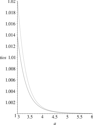
Figure 1: Plot of the ratios $R_{sq,q;(2,1)/(1,1)}$ (lower curve) and $R_{sq,q;(3,1)/(1,1)}$ (upper curve) as functions of $q$ for $3\leq q\leq 6$.

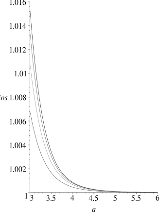
Figure 2: Plot of the ratios $R_{sq,q;(1,k)/(1,1)}$ for $k=2$ to $k=5$ as functions of $q$ for $3\leq q\leq 6$. From bottom to top, the curves refer to $k=2$, $k=3$, $k=4$, and $k=5$, respectively.

As the results in these figures show, our new lower bounds improve most on the earlier $W(sq,q)_{\ell;1,1}$ in the region of $q\mathrel{\raisebox{-2.58334pt}{$\stackrel{{\scriptstyle\textstyle>}}{{\sim}}$}}3$; as $q$ increases beyond this region, the new bounds approach the earlier one. This feature will be evident from the large-$q$ (small-$y$) expansions, since the new bound and the earlier one coincide in the terms of the small-$y$ expansion up to $O(y^{6})$. We also find this type of behavior for the new lower bounds that we have derived for other lattices; that is, the degree of improvement is greatest for the region of moderate $q$ slightly above $\chi(\Lambda)$. On a given lattice $\Lambda$, for larger $q$, our new bounds rapidly approach the earlier one with $k=1$ and $b=1$; i.e., the ratio $R_{\Lambda,q;(b,k)/(1,1)}$ rapidly approaches unity.

Combining these results with the results in Table I in ww and Table I in w3 , it follows that as $q$ increases above the interval of $q=3$ and $q=4$, these lower bounds approach extremely close to the actual respective values of $W(sq,q)$. As was evident from these tables in ww ; w3 , in the range $q\geq 3$, the greatest deviation of the lower bound $W(sq,q)_{\ell;1,1}$ from the actual value of $W(sq,q)$ occurs at $q=3$. It is thus of interest to determine how much closer our improved lower bounds are to $W(sq,3)$. From our general expression for $W(sq,q)_{\ell;1,2}$, we calculate the $q=3$ value

$$W(sq,3)_{\ell;1,2}{}\Big{|}_{q=3}=\frac{\sqrt{5+\sqrt{17}}}{2}=1.510223959...$$ (61)

so that

$$R_{sq,3;\ell;1,2} \equiv \frac{W(sq,3)_{\ell;1,2}{}\Big{|}_{q=3}}{W(sq,3)}$$ (62)

$$= \frac{3\sqrt{3(5+\sqrt{17})}}{16}=0.9809192...$$ (64)

This ratio and the other ones discussed here are listed in Table 1.

V Triangular Lattice

V.1 $b=1$, $k=1$

Since $W(tri,3)=1$ is exactly known, we will restrict our consideration of lower bounds to the range $q\geq 4$. We recall that for $b=1$ and $k=1$, one has the lower bound ww -wn $W(tri,q)\geq W(tri,q)_{\ell;1,1}$, where

$$W(tri,q)_{\ell;1,1}=\frac{(q-2)^{2}}{q-1}\ .$$ (65)

As was discussed in ww , $q$ increases beyond the lowest values above $\chi(tri)=3$, this lower bound rapidly approaches the known value of $W(tri,q)$ (see Table I in ww ), where the latter was determined by a numerical evaluation of an integral representation and infinite product expression baxter87 . For example, for $q=5,\ 6,\ 7$, $R_{tri,q;1,1}$ is equal to 0.9938, 0.9988, and 0.9996, respectively, and it increases monotonically with larger $q$. Since our new lower bounds on $W(tri,q)$ are more restrictive than (65), they are therefore even closer to the respective actual values of $W(tri,q)$.

The corresponding lower bound on $\overline{W}(tri,y)$ is $\overline{W}(tri,y)\geq\overline{W}(tri,y)_{\ell;1,1}$, where

$$\overline{W}(tri,y)_{\ell;1,1}=(1-y^{2})^{2}$$ (66)

(see Table III in wn ).

V.2 $b=2,\ 3$, $k=1$

Here we derive a new lower bound on $W(tri,q)$ using our first generalization of the CCM method with $b=2$, $k=1$. For this purpose, we need the chromatic polynomial of the cyclic strip of the triangular lattice of width $L_{y}=3$ vertices and arbitrary length, $L_{x}$. This was calculated in t . The dominant $\lambda$ in (16) is

$$\lambda_{tri,3,0,1}=\frac{1}{2}\bigg{[}q^{3}-7q^{2}+18q-17$$ (67)

$$+ \Big{[}q^{6}-14q^{5}+81q^{4}-250q^{3}+442q^{2}-436q+193\Big{]}^{1/2}\ \bigg{]}\ .$$ (69)

Combining this with $\lambda_{tri,2,0,1}=(q-2)^{2}$, we derive the lower bound

$$W(tri,q)\geq W(tri,q)_{\ell;2,1}\ ,$$ (72)

where

$$W(tri,q)_{\ell;2,1}=\frac{\lambda_{tri,3,0,1}}{\lambda_{tri,2,0,1}}=\frac{\bigg{[}q^{3}-7q^{2}+18q-17+\Big{[}q^{6}-14q^{5}+81q^{4}-250q^{3}+442q^{2}-436q+193\Big{]}^{1/2}\ \bigg{]}}{2(q-2)^{2}}\ .$$ (73)

The reduced function $\overline{W}(tri,y)$ is given by Eq. (12) with $\Lambda=tri$ and $\Delta=6$. The corresponding lower bound is

$$\overline{W}(tri,y)\geq\overline{W}(tri,y)_{\ell;2,1}\ ,$$ (74)

where

$$\overline{W}(tri,y)_{\ell;2,1}=\frac{(1+y)^{2}\bigg{[}1-4y+7y^{2}-5y^{3}+\Big{[}1-8y+26y^{2}-46y^{3}+53y^{4}-42y^{5}+17y^{6}\Big{]}^{1/2}\ \bigg{]}}{2(1-y)^{2}}\ .$$ (75)

Our new lower bound $W(tri,q)_{\ell;2,1}$ is larger than, and hence more restrictive than the previous lower bound, $W(tri,q)_{\ell;1,1}$. That is, from the analytic forms (66) and (75), we have proved that (for $q\geq 4$)

$$R_{tri,q;(2,1)/(1,1)}>1\ .$$ (76)

This ratio approaches 1 as $q\to\infty$.

As was evident in Table I in ww , the deviation of $W(tri,q)_{\ell;1,1}$ from the actual value of $W(tri,q)$ was greatest for $q=4$. Hence, it is of interest to determine how much closer our new lower bound $W(tri,q)_{\ell;2,1}$ is to the $W(tri,q)$ for this value, $q=4$. A closed-form integral representation has been given for $W(tri,q)$ baxter87 ; in particular, an explicit result is the value for $q=4$:

$$W(tri,4)=\frac{3\Gamma(1/3)^{3}}{4\pi^{2}}=\frac{2\pi}{\sqrt{3}\,\Gamma(2/3)^{3}}=1.460998486...$$ (77)

where the equivalence follows from the relation
$\Gamma(z)\Gamma(1-z)=\pi/\sin(\pi z)$ for the Euler Gamma function. We recall that

$$W(tri,4)_{\ell;1,1}=\frac{4}{3}$$ (78)

so

$$R_{tri,4;\ell;1,1}=\frac{2\Gamma(2/3)^{3}}{\sqrt{3}\,\pi}=0.9126178746...$$ (79)

(see Table I of ww ). The value of our new lower bound at $q=4$ is

$$W(tri,4)_{\ell;2,1}=\frac{7+\sqrt{17}}{8}=1.3903882...$$ (80)

so

$$R_{tri,4;\ell;2,1}=\frac{(7+\sqrt{17}\,)\sqrt{3}\,\Gamma(2/3)^{3}}{16\pi}=0.951669845...$$ (81)

We have also calculated the lower bound $W(tri,q)_{\ell;b,1}$ for $b=3$ and evaluated this for $q=4$. For reference, we list the various ratios $R_{tri,4;\ell;b,k}$ in Table 2. We see that $W(tri,4)_{\ell;2,1}$ and $W(tri,4)_{\ell;3,1}$ are closer to the exact value of $W(tri,4)$ than $W(tri,4)_{\ell;1,1}$.

V.3 $b=1$, $2\leq k\leq 5$

By the same means as above, we derive

$$W(tri,q)\geq W(tri,q)_{\ell;1,2}\ ,$$ (82)

with

$$W(tri,q)_{\ell;1,2}=\bigg{[}\frac{\lambda_{tri,3,0,1}}{q-1}\bigg{]}^{1/2}\ ,$$ (83)

where $\lambda_{tri,3,0,1}$ was given in Eq. (LABEL:lamtri3_dom). Equivalently,

$$\overline{W}(tri,y)\geq\overline{W}(tri,y)_{\ell;1,2}\ ,$$ (84)

where

$$\overline{W}(tri,y)_{\ell;1,2}=\frac{1}{\sqrt{2}}\,(1+y)^{2}\,\bigg{[}1-4y+7y^{2}-5y^{3}+\Big{[}1-8y+26y^{2}-46y^{3}+53y^{4}-42y^{5}+17y^{6}\Big{]}^{1/2}\ \bigg{]}^{1/2}\ .$$ (85)

For $b=1$, $k=3$, we need the dominant $\lambda$ in the chromatic polynomial for the cyclic strip of the triangular lattice of width $L_{y}=k+1=4$, namely, $\lambda_{tri,4,0,1}$. This chromatic polynomial was calculated in t , and the dominant $\lambda$ is given as the largest root of the quartic equation (227) in Appendix C. This is also the dominant $\lambda$ in the chromatic polynomial of the free strip of the triangular lattice with width $L_{y}=4$ and arbitrary length strip . We have also calculated $W(tri,q)_{\ell;1,k}$ for $k=4,\ 5$. For reference, we list the various ratios $R_{tri,4;\ell;1,k}$ in Table 2.

V.4 Plots

In Fig. 3 we plot the ratios $R_{tri,q;(b,1)/(1,1)}$ for $b=2$ and $b=3$ as functions of $q$ in the range $4\leq q\leq 6$, and in Fig. 4 we plot the ratios $R_{tri,q;(1,k)/(1,1)}$ for $k=2$ up to $k=5$, as functions of $q$ in same range. As with the square lattice, these plots illustrate the result that we have proved in general, that, for a given $q$, $R_{\Lambda,q;(1,k)/(1,1)}$ is an increasing function of $k$, and also our result that $R_{tri,q;(3,1)/(1,1)}\geq R_{tri,q;(2,1)/(1,1)}$.

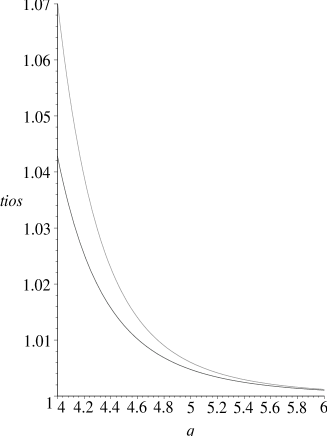
Figure 3: Plot of the ratios $R_{tri,q;(2,1)/(1,1)}$ (lower curve) and $R_{tri,q;(3,1)/(1,1)}$ (upper curve) as functions of $q$ for $4\leq q\leq 6$.

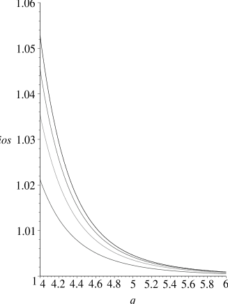
Figure 4: Plot of the ratios $R_{tri,q;(1,k)/(1,1)}$ for $k=2$ to $k=5$ as functions of $q$ for $4\leq q\leq 6$. From bottom to top, the curves refer to $k=2$, $k=3$, $k=4$, and $k=5$, respectively.

VI Honeycomb Lattice

Since $W(hc,2)=1$ is exactly known, we restrict our consideration of lower bounds for the honeycomb lattice to the range $q\geq 3$. We recall that for $b=1$ and $k=1$, one has the lower bound $W(hc,q)\geq W(hc,q)_{\ell;1,1}$, where w3

$$W(hc,q)_{\ell;1,1}=\frac{(D_{6})^{1/2}}{q-1}=\frac{(q^{4}-5q^{3}+10q^{2}-10q+5)^{1/2}}{q-1}\ ,$$ (86)

where the general expression for $D_{n}$ is given in Eq. (217). Ref. w3 noted that as $q$ increases beyond the lowest values above $\chi(hc)=2$, this lower bound rapidly approaches the actual value of $W(hc,q)$ (see Table I in w3 ), where the latter was determined by a Monte-Carlo simulation checked for larger $q$ with a large-$q$ series approximation. For example, for example, for $q=3,\ 4,\ 5$, $R_{hc,q;1,1}$ is equal to 0.99898, 0.99985, and 0.99996, respectively, and it increases monotonically with larger $q$. Since our new lower bounds on $W(hc,q)$ are more restrictive than (86), they are therefore even closer to the respective actual values of $W(hc,q)$.

The corresponding lower bound on $\overline{W}(hc,y)$ is $\overline{W}(hc,y)\geq\overline{W}(hc,y)_{\ell;1,1}$, where wn

$$\overline{W}(hc,y)_{\ell;1,1}=(1+y^{5})^{1/2}$$ (87)

(see Table III in wn ).

For the calculation of $W(hc,q)_{\ell;2,1}$, we need the chromatic polynomial of the cyclic strip of the honeycomb lattice of width $L_{y}=2b-1=3$ vertices and arbitrary length, $L_{x}$, in particular, the dominant $\lambda$. This $\lambda_{hc,3,0,1}$ is the largest (real) root of the cubic equation (230) in Appendix C hca . This dominant $\lambda$ is also the input that we need for the calculation of $W(hc,q)_{\ell;1,2}$, since the latter requires the same chromatic polynomial of the cyclic strip of the honeycomb lattice of width $L_{y}=k+1=3$ vertices and arbitrary length, $L_{x}$, in particular, the dominant term. This $\lambda$ is also the dominant term in the chromatic polynomial of the strip of the honeycomb lattice of width $L_{y}=3$ vertices and arbitrary length, with free boundary conditions strip .

VII $4\cdot 8^{2}$ Lattice

Using the CCM method with $b=1$ and $k=1$, Ref. w3 derived the lower bound $W((4\cdot 8^{2}),q)\geq W((4\cdot 8^{2}),q)_{\ell;1,1}$, where

$$W((4\cdot 8^{2})),q)_{\ell;1,1}=\frac{(D_{4}D_{8})^{1/4}}{q-1}\ .$$ (88)

Equivalently, $\overline{W}((4\cdot 8^{2}),y)>\overline{W}((4\cdot 8^{2}),y)_{\ell;1,1}$, where

$$\overline{W}((4\cdot 8^{2}),y)_{\ell;1,1}=[(1+y^{3})(1+y^{7})]^{1/4}\ .$$ (89)

We have obtained the slightly more restrictive lower bound $W((4\cdot 8^{2}),q)\geq W((4\cdot 8^{2}),q)_{\ell;1,2}$, where

$$W((4\cdot 8^{2}),q)_{\ell;1,2}=\bigg{[}\frac{\lambda_{(4\cdot 8^{2}),3,0,1}}{q-1}\bigg{]}^{1/3}\ ,$$ (90)

where $\lambda_{(4\cdot 8^{2}),3,0,1}$ is the largest (real) root of the cubic equation (239) in Appendix C. Correspondingly, $\overline{W}((4\cdot 8^{2}),y)\geq\overline{W}((4\cdot 8^{2}),y)_{\ell;1,2}$. We analyze the small-$y$ expansion of $\overline{W}((4\cdot 8^{2}),y)_{\ell;1,2}$ below.

VIII $3\cdot 6\cdot 3\cdot 6$ (kagomé) Lattice

In this section we consider the $(3\cdot 6\cdot 3\cdot 6)$ lattice, commonly called the kagomé lattice (which we shall abbreviate as $kag$). Using the CCM method with $b=1$ and $k=1$, Ref. wn derived the lower bound $W(kag,q)\geq W(kag,q)_{\ell;1,1}$, where

$$W(kag,q)_{\ell;1,1}=\frac{D_{3}^{2/3}D_{6}^{1/3}}{q-1}\ .$$ (91)

Equivalently, $\overline{W}(kag,y)>\overline{W}(kag,y)_{\ell;1,1}$, where wn

$$\overline{W}(kag,y)_{\ell;1,1}=(1-y^{2})^{2/3}(1+y^{5})^{1/3}\ .$$ (92)

The zigzag path used in the derivation of this lower bound was described in detail in Ref. wn .

Figure 5: Section of the $(3\cdot 6\cdot 3\cdot 6)$ (kagomé) lattice.

Here, we again take $b=1$ and $k=1$ but use a different type of path. A section of the kagomé lattice is shown in Fig. 5. Rather than the zigzag path used in wn , we choose the path to be given horizontal line in Fig. 5. The matrix $T$ then links the proper $q$-coloring of the vertices on this line, the vertices between this line and, say, the line above it, and the vertices on this higher-lying horizontal line. It turns out that the use of this different path yields a slightly more restrictive lower bound, which we shall indicate with a prime, namely $W(kag,q)\geq W(kag,q)_{\ell;1,1}^{\prime}$, where

$$W(kag,q)_{\ell;1,1}^{\prime}=$$ (93)

(94)

$$\Bigg{[}\frac{(q-2)\bigg{[}q^{4}-6q^{3}+14q^{2}-16q+10+\Big{[}q^{8}-12q^{7}+64q^{6}-200q^{5}+404q^{4}-548q^{3}+500q^{2}-292q+92\Big{]}^{1/2}\bigg{]}}{2(q-1)^{2}}\Bigg{]}^{1/3}\ .$$ (95)

(96)

(97)

Equivalently, we have $\overline{W}(kag,y)\geq\overline{W}(kag,y)_{\ell;1,1}^{\prime}$, where

$$\overline{W}(kag,y)_{\ell;1,1}^{\prime}=$$ (98)

(99)

$$2^{-1/3}(1+y)\Bigg{[}(1-y)\bigg{[}1-2y+2y^{2}-2y^{3}+3y^{4}+\Big{[}1-4y+8y^{2}-12y^{3}+14y^{4}-16y^{5}+16y^{6}-12y^{7}+9y^{8}\Big{]}^{1/2}\bigg{]}\Bigg{]}^{1/3}\ .$$ (100)

(101)

(102)

We find that

$$W(kag,q)_{\ell;1,1}^{\prime}\geq W(kag,q)_{\ell;1,1}$$ (103)

The fact that the use of a different path can yield a more restrictive bound with the same value of $b$ and $k$ was already shown for the honeycomb lattice in ww ; w3 . Thus, both Ref. w3 and Ref. ww used the CCM method with $b=1$ and $k=1$, but Ref. w3 obtained a more restrictive lower bound for the honeycomb lattice by using a different path. The bounds $W(kag,q)_{\ell;1,1}$ and $W(kag,q)_{\ell;1,1}^{\prime}$ both rapidly approach the actual value of $W(kag,q)$ as $q$ increases beyond the chromatic number, $\chi(kag)=3$. Below we shall show how the slight improvement with the new bound is manifested in the respective small-$y$ expansions of $W(kag,q)_{\ell;1,1}$ and $W(kag,q)_{\ell;1,1}^{\prime}$. In passing, we note that we have also studied generalizations of the CCM method for some other Archimedean lattices.

IX $sq_{d}$ Lattice

So far, we have considered planar lattices. The coloring compatibility matrix method and our generalizations of it, also apply to a subclass of nonplanar lattices, namely the subclass that can be constructed starting from a planar lattice and adding edges between vertices on the original planar lattice. An example of this is the $sq_{d}$ lattice. As noted above, the $sq_{d}$ lattice is formed from the square lattice by adding edges (bonds) connecting the two sets of diagonal next-nearest-neighbor vertices in each square. Thus, the vertices and edges in each square form a $K_{4}$ graph. (Here, the $K_{N}$ graph is the graph with $N$ vertices such that each vertex is connected to every other vertex by one edge.) Although an individual $K_{4}$ graph is planar, the $sq_{d}$ lattice is nonplanar. This lattice has coordination number $\Delta_{sq_{d}}=8$ and chromatic number $\chi(sq_{d})=4$. Although it is not 4-partite, an analysis of the way in which the number of proper 4-colorings of the vertices of a section of the $sq_{d}$ lattice grows with its area shows that $W(sq_{d},4)=1$.

Using the $b=1$, $k=1$ CCM, Ref. w3 derived the lower bound $W(sq_{d},q)\geq W(sq_{d},q)_{\ell;1,1}$, where

$$W(sq_{d},q)_{\ell;1,1}=\frac{\lambda_{sq_{d},2,0,1}}{\lambda_{C,0,1}}=\frac{(q-2)(q-3)}{q-1}\ .$$ (104)

IX.1 $b=2$, $k=1$

For our first generalization, namely $b=2$ and $k=1$, we need the dominant $\lambda$ for a cyclic strip of the $sq_{d}$ lattice of width $L_{y}=3$, which is k

$$\lambda_{sq_{d},3,0,1}=\frac{(q-3)}{2}\bigg{[}q^{2}-6q+11$$ (105)

$$+ \Big{[}q^{4}-12q^{3}+54q^{2}-112q+97\Big{]}^{1/2}\ \bigg{]}\ .$$ (107)

We thus derive the new lower bound $W(sq_{d},q)\geq W(sq_{d},q)_{\ell;2,1}$, where $W(sq_{d},q)_{\ell;2,1}=\lambda_{sq_{d},3,0,1}/\lambda_{sq_{s},2,0,1}$, i.e.,

$$W(sq_{d},q)_{\ell;2,1}=$$ (108)

(109)

$$\frac{q^{2}-6q+11+\Big{[}q^{4}-12q^{3}+54q^{2}-112q+97\Big{]}^{1/2}}{2(q-2)}\ .$$ (110)

(111)

(112)

From these explicit analytic results, we find

$$R_{sq_{d},q;(2,1)/(1,1)}>1\ .$$ (113)

That is, our new lower bound $W(sq_{d},q)_{\ell,2,1}$ is larger and hence more restrictive than the one obtained in w3 .

The corresponding lower bounds for the reduced $W$ functions are $\overline{W}(sq_{d},y)\geq\overline{W}(sq_{d},y)_{\ell;1,1}$, where

$$\overline{W}(sq_{d},y)_{\ell;1,1} = (1-y)(1-2y)(1+y)^{3}$$ (114)

$$= 1-4y^{2}-2y^{3}+3y^{4}+2y^{5}$$ (116)

and $\overline{W}(sq_{d},y)\geq\overline{W}(sq_{d},y)_{\ell;2,1}$, where

$$\overline{W}(sq_{d},y)_{\ell;2,1}=\frac{(1+y)^{3}\bigg{[}1-4y+6y^{2}+\Big{[}1-8y+24y^{2}-36y^{3}+28y^{4}\Big{]}^{1/2}\ \bigg{]}}{2(1-y)}\ .$$ (119)

IX.2 $b=1$, $k=2$

For $b=1$ and $k=2$, we derive the lower bound $W(sq_{d},q)\geq W(sq_{d},q)_{\ell;1,2}$, where

$$W(sq_{d},q)_{\ell;1,2}=\Big{[}\frac{\lambda_{sq_{d},3,0,1}}{\lambda_{C,0,1}}\Big{]}^{1/2}=\Bigg{[}\frac{(q-3)\Big{[}q^{2}-6q+11+\Big{(}q^{4}-12q^{3}+54q^{2}-112q+97\Big{)}^{1/2}\Big{]}}{2(q-1)}\Bigg{]}^{1/2}\ .$$ (120)

Equivalently, $\overline{W}(sq_{d},y)\geq\overline{W}(sq_{d},y)_{\ell;1,2}$, where

$$\overline{W}(sq_{d},y)_{\ell;1,2}=\frac{1}{\sqrt{2}}(1+y)^{3}\bigg{[}(1-2y)\Big{[}1-4y+6y^{2}+\Big{(}1-8y+24y^{2}-36y^{3}+28y^{4}\Big{)}^{1/2}\Big{]}\bigg{]}^{1/2}\ .$$ (121)

X Small-$y$ Expansions of New Lower Bounds

X.1 General

A lower bound on a function such as $W(\Lambda,q)$ or $\overline{W}(\Lambda,y)$ plays a role that is different from, and complementary to, that of a Taylor series expansion, in this case, a small-$y$ expansion. The lower bound is valid for any value of $q$ that is physical, but need not, a priori, be an accurate approximation to the actual function. In contrast, the large-$q$ (equivalently, small-$y$) Taylor series expansion is an approximation to the function itself and, within its radius of convergence, it satisfies the usual Taylor series convergence properties. Thus, if one truncates this series to a fixed order of expansion, then it becomes a progressively more accurate approximate as the expansion variable becomes smaller, and for a fixed value of the expansion variable, it becomes a more accurate expansion as one includes more terms.

A lower bound on a function $\overline{W}(\Lambda,y)$ need not, a priori, agree with the terms in the small-$y$ Taylor series expansion of this function. Some explicit examples of this are given in Appendix A. Interestingly, as discussed in ww -wn , the lower bounds derived there do agree with these small-$y$ series to a number of orders in $y$ (listed for Archimedean lattices in Table III and for the duals of Archimedean lattices in Table IV of Ref. wn ).

It is thus clearly of interest to carry out a similar comparison to determine the extent to which our new lower bounds, which we have shown improve upon those in biggs77 and ww -wn , agree with the respective small-$y$ expansions to higher order. We do this in the present section, showing that our new lower bounds are not only more stringent than the earlier ones, but also agree with the small-$y$ expansions of $\overline{W}(\Lambda,y)$ to higher order in $y$ than these earlier lower bounds.

Because $\overline{W}(\Lambda,y)_{\ell;b,k}$ is a lower bound on $\overline{W}(\Lambda,y)$, one can draw one immediate inference concerning the comparison of the small-$y$ Taylor series for these two functions, namely that for a given lattice $\Lambda$, if the small-$y$ Taylor series of $\overline{W}(\Lambda,y)_{\ell;b,k}$ coincides with the small-$y$ series for $\overline{W}(\Lambda,y)$ to order $O(y^{i_{c}})$, inclusive, then the difference

$$\overline{W}(\Lambda,y)-\overline{W}(\Lambda,y)_{\ell;b,k}=\kappa_{i_{c}+1}y^{i_{c}+1},\quad{\rm with}\ \kappa_{i_{c}+1}>0\ .$$ (122)

Thus, for example, with the $O(y^{i_{c}+1})$ term in $\overline{W}(\Lambda,y)$ denoted $w_{\Lambda,i_{c}+1}$ and with the $O(y^{i_{c}+1})$ term in $\overline{W}(\Lambda,y)_{\ell;b,k}$ denoted $w_{\Lambda;b,k;i_{c}+1}$, we have

$$w_{\Lambda;i_{c}+1}\geq w_{\Lambda;b,k;i_{c}+1}\ .$$ (123)

We discuss a subtlety in this comparison. One should first show that the small-$y$ expansion is, in fact, a Taylor series expansion, i.e., that $\overline{W}(\Lambda,y)$ is an analytic function at $y=0$ in the complex $y$ plane, or equivalently, that $W_{r}(\Lambda,q)$ is an analytic function at $1/q=0$ in the complex plane of the variable $1/q$. In fact, there are families of $N$-vertex graphs $G_{N}$ such that $W_{r}(\{G\},q)$ is not analytic at $1/q=0$ wa23 , where here $\{G\}$ denotes the formal limit $\lim_{N\to\infty}G_{N}$. This is a consequence of the property that the accumulation set of zeros of the chromatic polynomial $P(G_{N},q)$, denoted ${\cal B}$, extends to infinite $|q|$ in the $q$ plane, or equivalently, to the point $1/q=0$ in the $1/q$ plane. (The zeros of $P(G,q)$ are denoted as the chromatic zeros of $G$.) Refs. wa23 constructed and analyzed various families of graphs for which this is the case. For regular (vertex-transitive) $N$-vertex graphs $G_{\Lambda,N}$ of a lattice $\Lambda$ with either free or periodic (or twisted periodic) boundary conditions, the resultant $W_{r}(\Lambda,q)$ functions obtained in the $N\to\infty$ limit are analytic at $1/q=0$. This follows because a necessary condition that ${\cal B}$ extends to infinitely large $|q|$ as $N\to\infty$ is that the chromatic zeros of $G_{\Lambda,N}$ have magnitudes $|q|\to\infty$ in this limit. However, a vertex-transitive graph $G$ has the property that all vertices have the same degree, $\Delta$ and a chromatic zero of $G$ has a magnitude bounded above as $|q|<8.4\Delta$ sokalbound . So for the $N\to\infty$ limit of a regular lattice graph $\Lambda$, $W_{r}(\Lambda,q)$ is analytic at $1/q=0$ and equivalently, $\overline{W}(\Lambda,y)$ is analytic at $y=0$, and the corresponding series expansions in powers of $1/q$ and powers of $y$ are Taylor series expansions.

X.2 Square Lattice

The small-$y$ expansion of $\overline{W}(sq,y)$ is kimenting

$$\overline{W}(sq,y)=1+y^{3}+y^{7}+3y^{8}+4y^{9}+3y^{10}$$ (124)

$$+ 3y^{11}+O(y^{12})\ .$$ (126)

This series and several others for regular lattices are known to higher order than we list; we only display the various series up to the respective orders that are relevant for the comparison with our lower bounds. As is evident from Eq. (36), the previous lower bound $\overline{W}(sq,y)_{\ell;1,1}=1+y^{3}$ biggs77 coincides with the small-$y$ series to $O(y^{6})$, inclusive.

We list below the small-$y$ expansions of the various new lower bound functions $\overline{W}(sq,y)_{\ell;b,k}$ that we have derived with $b\geq 2$ and $k=1$ and with $b=1$, $k\geq 2$:

$$\overline{W}(sq,y)_{\ell;2,1}=1+y^{3}+y^{7}+3y^{8}+3y^{9}+O(y^{10})$$ (127)

(128)

(129)

$$\overline{W}(sq,y)_{\ell;1,2}=1+y^{3}+\frac{1}{2}y^{7}+\frac{3}{2}y^{8}+\frac{3}{2}y^{9}+O(y^{10})$$ (130)

(131)

(132)

and

$$\overline{W}(sq,y)_{\ell;1,3}=1+y^{3}+\frac{2}{3}y^{7}+2y^{8}+\frac{7}{3}y^{9}+O(y^{10})\ .$$ (133)

(134)

(135)

Comparing the small-$y$ expansion of our new lower bound function $\overline{W}(sq,y)_{\ell;b,1}$ with $b=2$, as well as the old lower bound function $\overline{W}(sq,y)_{\ell;1,1}$, with the actual small-$y$ series for $\overline{W}(sq,y)$ in Eq. (126), we can make several observations. First, the small-$y$ expansions for $\overline{W}(sq,y)_{\ell;2,1}$ coincides with the small-$y$ expansion of $\overline{W}(sq,y)$ to $O(y^{8})$, inclusive, which is an improvement by two orders in powers of $y$ as compared with $\overline{W}(sq,y)_{\ell;1,1}$ (see Eq. (36)). Since increasing $b$ (with $k$ fixed) improves the accuracy of the lower bound, it follows that $\overline{W}(sq,y)_{\ell;b,1}$ will also coincide with the series for $\overline{W}(sq,y)$ to at least $O(y^{8})$ for $b\geq 3$ as well as for $b=2$. Moreover, although the respective coefficients of $y^{9}$ in the series for $\overline{W}(sq,y)_{\ell;1,1}$ and $\overline{W}(sq,y)_{\ell;2,1}$, namely 0 and 3, do not match the coefficient of $y^{9}$ in the actual small-$y$ expansion of $\overline{W}(sq,y)$, which is 4, one can see that as $b$ increases from 1 to 2, this coefficient of the $y^{9}$ term increases toward the exact coefficient.

Regarding the matching of terms in the small-$y$ expansions of the $\overline{W}(sq,y)_{\ell;b,1}$, as compared with $\overline{W}(sq,y)_{\ell;1,k}$, that we have calculated, we find that this matching is better by two orders for the $\overline{W}(sq,y)_{\ell;b,1}$ than $\overline{W}(sq,y)_{\ell;1,k}$. That is, for the $k$ values that we have calculated, namely $k=2,\ 3$, the lower bounds $\overline{W}(sq,y)_{\ell;1,k}$ match the small-$y$ expansion of $\overline{W}(sq,y)$ to order $O(y^{6})$, the same order as $\overline{W}(sq,y)_{\ell;1,1}$.

A related property of our lower bounds for a general lattice $\Lambda$ and, in particular, for the square lattice, follows as a consequence of the theorem (24) and (25): with $b=1$, since the lower bound $\overline{W}(\Lambda,y)_{\ell;1,k}$ is a monotonically increasing function of $k$, the degree of matching of coefficients in the small-$y$ expansion for $\overline{W}(\Lambda,y)$ must improve monotonically as $k$ is increased. A priori, this improvement could be manifested in two ways (or a combination of the two): (i) as $k$ is increased, coefficients of terms of higher order in $y$ are exactly matched, or (ii) the coefficient of a given term of a certain order in $y$ approaches monotonically toward the exact value. For the present lattice $\Lambda=sq$, we see that, for the $\overline{W}(sq,q)_{\ell;1,k}$ that we have calculated, the latter type of behavior, (ii), occurs. That is, as we increase $k$ from 1 to 2 to 3, the coefficient of the $y^{7}$ term in the small-$y$ series for $\overline{W}(sq,y)_{\ell;1,k}$ increases from 0 to 1/2 to 2/3, moving toward the exact value of 1. This is similar to the behavior that we observed with the respective coefficients of the $y^{9}$ term in the small-$y$ expansions of $\overline{W}(sq,y)_{\ell;b,1}$ as compared with the exact value. This type of behavior is in accord with the inequality (123).

Regarding the relative ordering of the various lower bounds that we have obtained, from the small-$y$ expansion, we find, for large $q$, the ordering

$$\overline{W}(sq,y)>\overline{W}(sq,y)_{\ell;3,1}>\overline{W}(sq,y)_{\ell;2,1}$$ (136)

$$> \overline{W}(sq,y)_{\ell;1,3}>\overline{W}(sq,y)_{\ell;1,2}>\overline{W}(sq,y)_{\ell;1,1}\ .$$ (138)

In fact, we find that this ordering also extends down to the lowest value where we apply our lower bounds, namely $q=3$. For bounds on $W(sq,4)$ and $W(sq,5)$, see lm .

X.3 Triangular Lattice

The small-$y$ expansion of $\overline{W}(tri,y)$ is kimenting

$$\overline{W}(tri,y) = 1-2y^{2}+y^{4}+y^{5}+5y^{6}+16y^{7}+47y^{8}$$ (141)

$$+ 134y^{9}+O(y^{10})\ .$$ (143)

As is evident from Eq. (66), the previous lower bound $\overline{W}(tri,y)_{\ell;1,1}=(1-y^{2})^{2}$ ww ; wn , matches the small-$y$ series to $O(y^{4})$, inclusive.

We list below the small-$y$ expansions of the various new lower bounds $\overline{W}(tri,y)_{\ell;b,k}$ that we have derived with $b\geq 2$ and $k=1$, and with $b=1$, $k\geq 2$:

$$\overline{W}(tri,y)_{\ell;2,1}=1-2y^{2}+y^{4}+y^{5}+5y^{6}+14y^{7}+O(y^{8})$$ (144)

(145)

(146)

$$\overline{W}(tri,y)_{\ell;1,2}=1-2y^{2}+y^{4}+\frac{1}{2}y^{5}+\frac{5}{2}y^{6}+O(y^{7})$$ (147)

(148)

(149)

and

$$\overline{W}(tri,y)_{\ell;1,3}=1-2y^{2}+y^{4}+\frac{2}{3}y^{5}+\frac{10}{3}y^{6}+O(y^{7})\ .$$ (150)

(151)

(152)

Comparing these with the small-$y$ series for $\overline{W}(tri,y)_{\ell;1,1}$, we find that, among (146)-(152), the greatest matching of terms is achieved with (146), i.e., by increasing $b$. Specifically, the small-$y$ expansion for $\overline{W}(tri,y)_{\ell;2,1}$ matches the small-$y$ expansion of $\overline{W}(tri,y)$ to $O(y^{6})$ inclusive, which is an improvement by two orders in $y$ as compared with $\overline{W}(tri,y)_{\ell;1,1}$. This increase by two orders in $y$ is the same amount of improvement that we found for our lower bound for the square lattice, $\overline{W}(sq,y)_{\ell;2,1}$ as compared with $\overline{W}(sq,y)_{\ell;1,1}$.

As was true of the lower bounds for the square lattice, the lower bounds $\overline{W}(tri,y)_{\ell;1,k}$ with $k=2$ and $k=3$ coincide with the small-$y$ series for $\overline{W}(tri,y)$ to the same order, namely $O(y^{4})$, as $\overline{W}(tri,y)_{\ell;1,1}$. However, as $k$ increases from 1 to 2 to 3, the coefficient of the first unmatched term in the respective small-$y$ series for $\overline{W}(tri,y)_{\ell;1,k}$, viz., the $y^{5}$ term, increases from 0 to 1/2 to 2/3, moving toward the exact value of 1. An inequality that follows from the theorem (24) and general result (25), is that with $b=1$, $\overline{W}(tri,y)_{\ell;1,k}$ is a monotonically increasing function of $k$.

Concerning the relative ordering of the various lower bounds that we have obtained, from the small-$y$ expansion, we find, for large $q$, the ordering

$$\overline{W}(tri,y)>\overline{W}(tri,y)_{\ell;2,1}>\overline{W}(tri,y)_{\ell;1,3}>$$ (153)

$$> \overline{W}(tri,y)_{\ell;1,2}>\overline{W}(tri,y)_{\ell;1,1}\ .$$ (155)

Indeed, we find that this ordering also extends down to the lowest value where we apply our bounds, namely $q=4$.

X.4 Honeycomb Lattice

The small-$y$ expansion of $\overline{W}(hc,y)$ is kimenting

$$\overline{W}(hc,y) = 1+\frac{1}{2}y^{5}-\frac{1}{2^{3}}y^{10}+y^{11}+2y^{12}+\frac{3}{2}y^{13}$$ (156)

$$+ y^{14}-\frac{15}{2^{4}}y^{15}+O(y^{16})\ .$$ (158)

The previous lower bound $\overline{W}(hc,y)_{\ell;1,1}=(1+y^{5})^{1/2}$ ww -wn has the small-$y$ expansion

$$\overline{W}(hc,y)_{\ell;1,1}=1+\frac{1}{2}y^{5}-\frac{1}{2^{3}}y^{10}+\frac{1}{2^{4}}y^{15}+O(y^{20})\ .$$ (159)

(160)

(161)

Thus, as was noted in ww -wn , this small-$y$ expansion coincides with the small-$y$ expansion of $\overline{W}(hc,y)$ to the quite high order $O(y^{10})$.

We list below the small-$y$ expansions of the various new lower bound functions $\overline{W}(hc,y)_{\ell;b,k}$ that we have derived with $b\geq 2$ and $k=1$ and with $b=1$, $k\geq 2$:

$$\overline{W}(hc,y)_{\ell;2,1}=1+\frac{1}{2}y^{5}-\frac{1}{2^{3}}y^{10}+y^{11}+2y^{12}+y^{13}+O(y^{15})$$ (162)

and

$$\overline{W}(hc,y)_{\ell;1,2}=1+\frac{1}{2}y^{5}-\frac{1}{2^{3}}y^{10}+\frac{1}{2}y^{11}+y^{12}+O(y^{13})\ .$$ (163)

As with the square and triangular lattices, we find that among (162)-(163), the greatest matching of terms is achieved with (162), i.e., by increasing $b$. Specifically, the small-$y$ expansion for $\overline{W}(hc,y)_{\ell;2,1}$ matches the small-$y$ expansion of $\overline{W}(hc,y)$ to $O(y^{12})$ inclusive, which is an improvement by two orders in $y$ as compared with $\overline{W}(hc,y)_{\ell;1,1}$.

The theorem (24) and corollary (25) imply that $W(hc,q)_{\ell;1,2}>W(hc,q)_{\ell;1,1}$, and this inequality is reflected in the degree of matching of the small-$y$ expansions for the corresponding functions $\overline{W}(hc,y)_{\ell;1,2}$ and $\overline{W}(hc,y)_{\ell;1,1}$. Although $\overline{W}(hc,y)_{\ell;1,2}$ does not increase the order of matching, as compared with $\overline{W}(hc,y)_{\ell;1,1}$, it begins the process of building up a nonzero coefficient for a $y^{11}$ term, which was zero in the expansion of $\overline{W}(hc,y)_{\ell;1,1}$. Specifically, the small-$y$ expansion of $\overline{W}(hc,y)_{\ell;1,2}$ contains a $y^{11}$ term with coefficient 1/2, building toward the exact coefficient, 1, of $y^{11}$ in (158).

X.5 $4\cdot 8^{2}$ Lattice

We next consider a (bipartite) heteropolygonal Archimedean lattice, namely the $(4\cdot 8^{2})$ lattice. The small-$y$ expansion of $\overline{W}((4\cdot 8^{2}),y)$ is w3 ; wn

$$\overline{W}((4\cdot 8^{2}),y) = 1+\frac{1}{4}y^{3}-\frac{3}{2^{5}}y^{6}+\frac{1}{4}y^{7}+\frac{7}{2^{7}}y^{9}$$ (164)

$$+ \frac{1}{2^{4}}y^{10}-\frac{77}{2^{11}}y^{12}+O(y^{13})\ .$$ (166)

The small-$y$ expansion of the lower bound obtained in ww ; wn , $\overline{W}((4\cdot 8^{2}),y)_{\ell;1,1}$, is

$$\overline{W}((4\cdot 8^{2}),y)_{\ell;1,1}=1+\frac{1}{4}y^{3}-\frac{3}{2^{5}}y^{6}+\frac{1}{4}y^{7}+\frac{7}{2^{7}}y^{9}$$ (167)

$$+ \frac{1}{2^{4}}y^{10}-\frac{77}{2^{11}}y^{12}-\frac{3}{2^{7}}y^{13}-\frac{3}{2^{5}}y^{14}+\frac{231}{2^{13}}y^{15}+O(y^{16})\ .$$ (169)

As was noted in w3 ; wn , this coincides with the small-$y$ expansion of $\overline{W}((4\cdot 8^{2}),y)$ to the quite high order $O(y^{12})$.

We list below the small-$y$ expansions of the various new lower bound functions $\overline{W}((4\cdot 8^{2}),y)_{\ell;b,k}$ that we have derived with $b\geq 2$ and $k=1$ and with $b=1$, $k\geq 2$:

$$\overline{W}((4\cdot 8^{2}),y)_{\ell;2,1}=1+\frac{1}{4}y^{3}-\frac{3}{2^{5}}y^{6}+\frac{1}{4}y^{7}$$ (172)

$$+ \frac{7}{2^{7}}y^{9}+\frac{1}{2^{4}}y^{10}-\frac{77}{2^{11}}y^{12}+\frac{189}{2^{7}}y^{13}+O(y^{14})$$ (174)

and

$$\overline{W}((4\cdot 8^{2}),y)_{\ell;1,2}=1+\frac{1}{4}y^{3}-\frac{3}{2^{5}}y^{6}+\frac{1}{4}y^{7}$$ (177)

$$+ \frac{7}{2^{7}}y^{9}+\frac{1}{2^{4}}y^{10}-\frac{77}{2^{11}}y^{12}+\frac{93}{2^{7}}y^{13}+\frac{45}{32}y^{14}+O(y^{15})\ .$$ (179)

Evidently, the small-$y$ series expansions of $\overline{W}((4\cdot 8^{2}),y)_{\ell;2,1}$ and $\overline{W}((4\cdot 8^{2}),y)_{\ell;1,2}$ match the small-$y$ expansion of $\overline{W}((4\cdot 8^{2}),y)$ to at least the same order as $\overline{W}((4\cdot 8^{2}),y)_{\ell;1,1}$. Further, we observe that for small-$y$,

$$\overline{W}((4\cdot 8^{2}),y)_{\ell;2,1}>\overline{W}((4\cdot 8^{2}),y)_{\ell;1,2}>\overline{W}((4\cdot 8^{2}),y)_{\ell;1,1}$$ (182)

X.6 $3\cdot 6\cdot 3\cdot 6$ (kagomé) Lattice

The small-$y$ expansion of $\overline{W}(kag,y)$ is wn

$$\overline{W}(kag,y)=1-\frac{2}{3}y^{2}-\frac{1}{3^{2}}y^{4}+\frac{1}{3}y^{5}$$ (183)

(184)

$$-\frac{4}{3^{4}}y^{6}-\frac{2}{3^{2}}y^{7}-\frac{7}{3^{5}}y^{8}+O(y^{9})\ .$$ (185)

As was discussed in wn , the small-$y$ expansion of the $b=1$, $k=1$ lower bound $\overline{W}(kag,y)_{\ell;1,1}$ derived there (listed above as Eq. (91)) coincides to $O(y^{8})$ with the small-$y$ series for the actual quantity $\overline{W}(kag,y)$. Explicitly,

$$\overline{W}(kag,y)_{\ell;1,1}=1-\frac{2}{3}y^{2}-\frac{1}{3^{2}}y^{4}+\frac{1}{3}y^{5}$$ (186)

(187)

$$-\frac{4}{3^{4}}y^{6}-\frac{2}{3^{2}}y^{7}-\frac{7}{3^{5}}y^{8}-\frac{1}{3^{3}}y^{9}-\frac{95}{3^{6}}y^{10}$$ (188)

(189)

$$+O(y^{11})\ .$$ (190)

Our new bound has the small-$y$ expansion

$$\overline{W}(kag,y)_{\ell;1,1}^{\prime}=1-\frac{2}{3}y^{2}-\frac{1}{3^{2}}y^{4}+\frac{1}{3}y^{5}$$ (191)

(192)

$$-\frac{4}{3^{4}}y^{6}-\frac{2}{3^{2}}y^{7}-\frac{7}{3^{5}}y^{8}+\frac{8}{3^{3}}y^{9}+\frac{634}{3^{6}}y^{10}$$ (193)

(194)

$$+O(y^{11})\ .$$ (195)

Thus,

$$\overline{W}(kag,y)_{\ell;1,1}^{\prime}-\overline{W}(kag,y)_{\ell;1,1}=\frac{1}{3^{2}}y^{9}+O(y^{10})\ .$$ (196)

One could derive similar lower bounds for other Archimedean lattices not considered here, e.g., the $3\cdot 12\cdot 12$ lattice wn ; tsai312 .

X.7 $sq_{d}$ Lattice

Since the lower bound $\overline{W}(sq_{d},y)_{\ell;1,1}$ derived in w3 and given above in Eq. (LABEL:wysqd_lbound_b1k1) is a polynomial, it is identical to its small-$y$ Taylor series expansion.

Expanding $\overline{W}(sq_{d},y)_{\ell;2,1}$, we find

$$\overline{W}(sq_{d},y)_{\ell;2,1}=1-4y^{2}-y^{3}+6y^{4}+5y^{5}+O(y^{6})\ .$$ (197)

(198)

(199)

Similarly,

$$\overline{W}(sq_{d},y)_{\ell;1,2}=1-4y^{2}-\frac{3}{2}y^{3}+\frac{9}{2}y^{4}+\frac{7}{2}y^{5}+O(y^{6})$$ (200)

(201)

(202)

$$\overline{W}(sq_{d},y)_{\ell;1,3}=1-4y^{2}-\frac{4}{3}y^{3}+5y^{4}+\frac{13}{3}y^{5}+O(y^{6})\ .$$ (203)

(204)

(205)

From these expansions we find, for large $q$, the ordering

$$\overline{W}(sq_{d},y)>\overline{W}(sq_{d},y)_{\ell;2,1}>\overline{W}(sq_{d},y)_{\ell;1,2}>\overline{W}(sq_{d},y)_{\ell;1,1}$$ (206)

This is the same ordering that we found for the other lattices.

XI Conclusions

Nonzero ground-state entropy per site, $S_{0}$, and the associated ground-state degeneracy per site, $W=e^{S_{0}/k_{B}}$, are of fundamental importance in statistical mechanics. In this paper we have presented generalized methods for deriving lower bounds on the ground-state degeneracy per site, $W(\Lambda,q)$, of the $q$-state Potts antiferromagnet on several different lattices $\Lambda$. Our first generalization is to consider a coloring compatibility matrix that relates a strip of width $b\geq 2$ vertices to an adjacent strip of the same width. Our second generalization is to consider a coloring compatibility matrix that acts $k\geq 2$ times in relating a path on $\Lambda$ to an adjacent parallel path. We have applied these generalizations to obtain new lower bounds on $W(\Lambda,q)$, denoted $W(\Lambda,q)_{\ell;b,k}$. In this notation, the lower bounds previously derived in ww -biggs77 have $b=1$ and $k=1$. One of the interesting properties of these bounds $W(\Lambda,q)_{\ell;1,1}$ obtained in ww -biggs77 was that as $q$ increases beyond $\chi(\Lambda)$ they rapidly approach quite close to the actual respective values of $W(\Lambda,q)$. We have shown that our new lower bounds are slightly more restrictive than these previous lower bounds, and consequently are even closer to the actual values $W(\Lambda,q)$. We have demonstrated how this is manifested in the matching to higher-order terms with the large-$q$ (small-$y$) Taylor series expansions for the corresponding functions $\overline{W}(\Lambda,y)$ for the various lattices that we have considered.

Appendix A $W(\Lambda_{rp.},q)$ at $q=\chi(\Lambda)$

We mention here a subtlety that results from the noncommutativity in the limits (14). An $r$-partite $rp.$ graph with $N$ vertices, $G_{rp.,N}$ has chromatic number $\chi(G_{rp.,N})=r$. One equivalent definition of an $r$-partite graph is that its chromatic polynomial, evaluated at $q=r$, satisfies

$$P(G_{rp.,N},r)=r!$$ (207)

The square and honeycomb lattices are bipartite (as are the $(4\cdot 6\cdot 12)$, and $(4\cdot 8\cdot 8)$ lattices, among Archimedean lattices), while the triangular lattice is tripartite (for others Archimedean lattices and their planar duals, see, e.g., Tables I and II in wn ). It follows that, with the $D_{Nq}$ definition for $W(\Lambda,q)$, namely setting $q=r$ and then taking the $N\to\infty$ limit in Eq. (2), one has

$$W(\Lambda_{rp.},r)=1\ .$$ (208)

As discussed in w , because of the noncommutativity (14), if instead of setting $q=r$, evaluating $P(G_{rp.},r)$, and then taking the $N\to\infty$, one first takes $N\to\infty$ with $q$ in the vicinity of $r$, and then performs the limit $q\to r$, one can, in general, get a different result for $W(\Lambda,q)$. Indeed, this is the case for many lattice strips of regular lattices of a fixed width $L_{y}$, an arbitrary length, $L_{x}$, and various transverse and longitudinal boundary conditions w ; wcy ; s4 ; t . The coloring problem on a given lattice $\Lambda$ is of interest for $q\geq\chi(\Lambda)$, since this is the minimum (integer) value of $q$ for which one can carry out a proper $q$-coloring of the vertices of $\Lambda$. In a number of cases, $\chi(\Lambda)<q_{c}(\Lambda)$. If one considers $W(\Lambda,q)$ for $q<q_{c}(\Lambda)$, then one must deal with the generic noncommutativity in the limits (14) w . Here we always use the order $D_{Nq}$, i.e., we fix $q$ to a given value and then take $N\to\infty$. Actually, in view of the results (207) and (208), for the square and honeycomb lattices, $W(sq,2)=W(hc,2)=1$, and for the triangular lattice, $W(tri,3)=1$. Since our new lower bounds are intended for practical use and since one already knows (with the $D_{Nq}$ definition) the values of $W(sq,2)$, $W(hc,2)$, and $W(tri,3)$ exactly, we may restrict our analysis to the application of our new bounds in the range $q\geq 3$ for the square and honeycomb lattices and to the range $q\geq 4$ for the triangular lattice.

For reference, we recall an elementary lower bound on $P(G,q)$ and hence on $\lim_{N\to\infty}P(G,q)^{1/N}$, where $G$ is an $N$-vertex graph. If $G$ is bipartite ($bp.$) then one can assign a color to all of the vertices of the even subgraph in any of $q$ ways and then one can assign one of the remaining $q-1$ colors to each of the vertices on the odd subgraph independently, so $P(G_{bp.},q)\geq q(q-1)^{N/2}$. Hence, for a bipartite lattice, denoting $\Lambda_{bp.}$ as the $N\to\infty$ limit of $G_{bp.}$, one has $W(\Lambda_{bp.},q)\geq(q-1)^{1/2}$. Both of these lower bounds are realized as equalities only in the case $q=2$. More generally, if $G_{rp.}$ is an $r$-partite graph and $\Lambda_{rp.}=\lim_{N\to\infty}\Lambda_{rp.,N}$, then

$$P(G_{rp.},q)\geq\Big{[}\prod_{s=0}^{r-2}(q-s)\Big{]}[q-(r-1)]^{N/r}$$ (209)

and hence

$$W(\Lambda_{rp.},q)\geq\ [q-(r-1)]^{1/r}\ .$$ (210)

Thus, for example, one has the elementary lower bounds $W(sq,q)\geq(q-1)^{1/2}$ and $W(tri,q)\geq(q-2)^{1/3}$, etc.

For $q>r$ on $\Lambda_{rp.}$, the lower bound (210) is less stringent than the ones derived in wn -biggs77 and here via coloring matrix methods. Indeed, these lower bounds illustrate the fact noted in the text, namely that, a priori, a lower bound need not agree with terms in the large-$q$ expansion of $W_{r}(\Lambda,q)$ or the equivalent small-$y$ expansion of $\overline{W}(\Lambda,y)$. For example, for the square and honeycomb lattices, the $r=2$ special cases of (210) read, for $q\geq 2$,

$$W(sq,q)\geq(q-1)^{1/2}$$ (211)

and

$$W(hc,q)\geq(q-1)^{1/2}\ .$$ (212)

Since $W(\Lambda,q)\sim q$ for large $q$, these lower bounds becomes progressively worse (i.e., farther from the actual value) as $q$ increases above 2. The corresponding lower bounds in terms of $\overline{W}(sq,y)$ and $\overline{W}(hc,y)$ are

$$\overline{W}(sq,y)\geq(1+y)\sqrt{y}$$ (213)

and

$$\overline{W}(hc,y)\geq\sqrt{y(1+y)}\ .$$ (214)

Rather than matching any terms in the respective small-$y$ expansions (126) and (158), the right-hand sides of these lower bounds vanish for small $y$. Similarly, since the triangular lattice is tripartite, the $r=3$ special case of (210) yields the lower bound, for $q\geq 3$,

$$W(tri,q)\geq(q-2)^{1/3}\ .$$ (215)

In terms of $\overline{W}(tri,y)$, this is

$$\overline{W}(tri,y)\geq y^{2/3}(1-y)^{1/3}(1+y)^{2}\ .$$ (216)

Again, for small $y$, this vanishes rather than matching any of the terms of the small-$y$ expansion (143). Thus, as noted, a lower bound need not match any of the terms in the small-$y$ expansion. This emphasizes how impressive the new lower bounds are in their matching of these terms in the small-$y$ expansions for the various lattices to high order.

Appendix B Lower Bounds $W(\Lambda,q)_{\ell;1,1}$ and $\overline{W}(\Lambda,y)_{\ell;1,1}$ for Archimedean Lattices

A number of general results were proved in Ref. wn concerning lower bounds which, in the notation of this paper, are $W(\Lambda,q)_{\ell;1,1}$ and $\overline{W}(\Lambda,y)_{\ell;1,1}$. These results in wn applied for all eleven Archimedean lattices. We have given the notation for an Archimedean lattice in the text. These lower bounds from wn are relevant here because we compare our new lower bounds $W(\Lambda,q)_{\ell;b,k}$ and the corresponding lower bounds $\overline{W}(\Lambda,y)_{\ell;b,k}$ with $b\geq 2$ and/or $k\geq 2$ to these earlier ones with $b=k=1$. (Ref. wn also gave lower bounds for the planar duals of the Archimedean lattices; we do not list these here but instead refer the reader to wn .)

The chromatic polynomial of a circuit graph is $P(C_{n},q)=(q-1)^{n}+(q-1)(-1)^{n}$. Since this chromatic polynomial has $q(q-1)$ as a factor, we can write it as $P(C_{n},q)=q(q-1)D_{n}(q)$, where

$$D_{n}(q)=\frac{P(C_{n},q)}{q(q-1)}=\sum_{s=0}^{n-2}(-1)^{s}{{n-1}\choose{s}}\,q^{n-2-s}\ .$$ (217)

Ref. wn proved the following general lower bounds for an Archimedean lattice, $\Lambda=(\prod_{i}p_{i}^{a_{i}})$ (where we add the subscripts $1,1$ to indicate $b=1$ and $k=1$ to match our current notation for $W(\Lambda,q)_{\ell;b,k}$):

$$W\Bigl{(}(\prod_{i}p_{i}^{a_{i}}),q\Bigr{)}\geq W\Bigl{(}(\prod_{i}p_{i}^{a_{i}}),q\Bigr{)}_{\ell;1,1}\ ,$$ (218)

where

$$W\Bigl{(}(\prod_{i}p_{i}^{a_{i}}),q\Bigr{)}_{\ell;1,1}=\frac{\prod_{i}D_{p_{i}}(q)^{\nu_{p_{i}}}}{q-1}\ ,$$ (219)

Here, the $\{i\}$ in the product label the set of $p_{i}$-gons involved in $\Lambda$ and $\nu_{p}$ (with $p=p_{i}$ here) was defined in Eq. (2.10) of wn .

This lower bound takes a somewhat simpler form in terms of the related function $\overline{W}(\Lambda,y)_{\ell}$, namely,

$$\overline{W}\Bigl{(}(\prod_{i}p_{i}^{a_{i}}),y\Bigr{)}\geq\overline{W}\Bigl{(}(\prod_{i}p_{i}^{a_{i}}),y\Bigr{)}_{\ell;1,1}\ ,$$ (220)

where

$$\overline{W}\Bigl{(}(\prod_{i}p_{i}^{a_{i}}),y\Bigr{)}_{\ell,1,1}=\prod_{i}\Bigl{[}1+(-1)^{p_{i}}y^{p_{i}-1}\Bigl{]}^{\nu_{p_{i}}}$$ (221)

A summary of these for Archimedean lattices is given in Table IV of wn .

Appendix C Higher-Degree Algebraic Equations for Certain $\lambda_{\Lambda,L_{y},0,1}$

In this appendix we list some algebraic equations of degree higher than 2 that are used in the text. The cubic equation whose largest (real) root is $\lambda_{sq,4,0,1}$, used for our lower bound $W(sq,q)_{\ell;1,3}$, is

$$\lambda^{3}-(q^{4}-7q^{3}+23q^{2}-41q+33)\,\lambda^{2}+(2q^{6}-23q^{5}+116q^{4}-329q^{3}+553q^{2}-517q+207)\,\lambda$$ (222)

$$- q^{8}+16q^{7}-112q^{6}+449q^{5}-1130q^{4}+1829q^{3}-1858q^{2}+1084q-279=0\ .$$ (224)

The quartic equation whose largest (real) root is $\lambda_{tri,4,0,1}$, used for our lower bound $W(tri,q)_{\ell;1,3}$, is

$$\lambda^{4}-(q^{4}-10q^{3}+42q^{2}-88q+76)\,\lambda^{3}+(q-2)(q-3)^{2}(3q^{3}-22q^{2}+60q-60)\,\lambda^{2}$$ (225)

$$- (q-2)^{2}(q-3)^{3}(3q^{3}-21q^{2}+51q-43)\,\lambda+(q-2)^{6}(q-3)^{4}=0\ .$$ (227)

The cubic equation whose largest (real) root is $\lambda_{hc,3,0,1}$ used in our lower bound $W(hc,q)_{\ell;2,1}$ is

$$\lambda^{3}-(q^{6}-8q^{5}+28q^{4}-56q^{3}+71q^{2}-58q+26)\,\lambda^{2}$$ (228)

$$+ (q-1)^{2}(q^{6}-10q^{5}+43q^{4}-102q^{3}+144q^{2}-120q+49)\,\lambda-(q-1)^{4}(q-2)^{2}=0\ .$$ (230)

The cubic equation whose largest (real) root is $\lambda_{(4\cdot 8^{2}),3,0,1}$, used in our bound $W((4\cdot 8^{2}),q)_{\ell;1,2}$ is

$$\lambda^{3}-(q^{12}-16q^{11}+120q^{10}-558q^{9}+1794q^{8}-4212q^{7}+7437q^{6}-10018q^{5}+10324q^{4}$$ (231)

(232)

$$-8064q^{3}+4648q^{2}-1854q+414)\,\lambda^{2}$$ (233)

(234)

$$+(q-1)^{4}(q^{12}-20q^{11}+188q^{10}-1094q^{9}+4375q^{8}-12640q^{7}+27033q^{6}-43164q^{5}$$ (235)

(236)

$$+51235q^{4}-44380q^{3}+26931q^{2}-10462q+2017)\,\lambda$$ (237)

(238)

$$-(q-1)^{8}(q-2)^{2}(q-3)^{2}(q^{2}-3q+3)^{2}=0\ .$$ (239)

Table 1: Values of $R_{sq,q;\ell;b,k}$ for $q=3$ and some illustrative values of $b$ and $k$.

$b$	$k$	$W(sq,3)_{\ell;b,k}$	$R_{sq,3;\ell;b,k}$
1	1	1.500000	0.974279
2	1	1.520518	0.987605
3	1	1.530340	0.993985
1	2	1.510224	0.980919
1	3	1.5162645	0.984843
1	4	1.520249	0.987430
1	5	1.523073	0.989265

Table 2: Values of $R_{tri,q;\ell;b,k}$ for $q=4$ and some illustrative values of $b$ and $k$.

$b$	$k$	$W(tri,4)_{\ell;b,k}$	$R_{tri,4;\ell;b,k}$
1	1	1.333333	0.912618
2	1	1.390388	0.951670
3	1	1.427052	0.976765
1	2	1.361562	0.931939
1	3	1.380569	0.944949
1	4	1.393923	0.954089
1	5	1.403672	0.960762

References

- (1) W. F. Giauque and J. W. Stout, J. Am. Chem. Soc. 58, 1144 (1936). Here, cal/(K-mole).
- (2) L. Pauling, J. Am. Chem. Soc. 57, 2680 (1935); L. Pauling, The Nature of the Chemical Bond (Cornell Univ. Press, Ithaca, 1960), p. 466.
- (3) B. A. Berg, C. Muguruma, and Y. Okamoto, Phys. Rev. B 75, 092202 (2007).
- (4) F. Y. Wu, Rev. Mod. Phys. 54, 235 (1982).
- (5) R. Shrock and S.-H. Tsai, Phys. Rev. E 55, 6791 (1997).
- (6) R. Shrock and S.-H. Tsai, Phys. Rev. E 56, 2733 (1997).
- (7) R. Shrock and S.-H. Tsai, Phys. Rev. E 56, 4111 (1997).
- (8) N. L. Biggs, Bull. London Math. Soc. 9, 54 (1977).
- (9) See, e.g., P. Lancaster and M. Tismenetsky, The Theory of Matrices, with Applications (New York, Academic Press, 1985); H. Minc, Nonnegative Matrices (New York, Wiley, 1988).
- (10) D. London, Duke Math. J. 33, 511 (1966).
- (11) Grünbaum, B. and Shephard, G. 1989 Tilings and Patterns: an Introduction (Freeman, New York, 1989).
- (12) R. Shrock and S.-H. Tsai, Phys. Rev. E55, 5165 (1997).
- (13) S.-C. Chang and R. Shrock, Physica A 296, 131 (2001).
- (14) R. Shrock and S.-H. Tsai, Phys. Rev. E 60, 3512 (1999); R. Shrock and S.-H. Tsai, Physica A 275, 429-449 (2000).
- (15) R. Shrock and S.-H. Tsai, J. Phys. A Letts. 32, L195 (1999).
- (16) R. Shrock, Phys. Lett. A 261, 57 (1999); Physica A 283, 388 (2000); Discrete Math. 231, 421 (2001).
- (17) S.-C. Chang and R. Shrock, Phys. Rev. E 62, 4650 (2000).
- (18) J. K. Merikoski, Linear Alg. and Applic. 60, 177 (1984).
- (19) M. Roček, R. Shrock, and S.-H. Tsai), Physica A 252, 505 (1998).
- (20) D. Kim and I. G. Enting, J. Combin. Theory, B 26, 327 (1979). Note that the function that Kim and Enting denoted for the honeycomb lattice is implicitly defined per 2-cell (hexagon), not per site, and hence is equal to .
- (21) As it must be, the lower bound is a positive real analytic function of in the relevant range of , namely, . We comment on its analytic structure. The poles from zeros in the denominator occur at and the branch-point singularities in the square root in the numerator occur where the factor vanishes, at , and at the two pairs of complex-conjugate zeros of the quartic factor, which are and , to the indicated floating-point accuracy. Similar comments apply for other explicit analytic expressions for lower bounds given in the text.
- (22) A. Lenard, unpublished, as cited in E. H. Lieb, Phys. Rev. 162, 162 (1967).
- (23) S.-C. Chang and R. Shrock, Physica A 290, 402 (2001).
- (24) S.-C. Chang and R. Shrock, Physica A 316, 335 (2002).
- (25) S.-C. Chang and R. Shrock, Ann. Phys. 290, 124 (2001).
- (26) R. J. Baxter, J. Phys. A 20, 5231 (1987).
- (27) S.-C. Chang and R. Shrock, Physica A 296, 183 (2001); J. Stat. Phys. 130, 1011 (2008).
- (28) R. Shrock and S.-H. Tsai, Phys. Rev. E56, 3935 (1997); J. Phys. A 31, 9641 (1998); Physica A 265, 186 (1999).
- (29) A. Sokal, Combin. Probab. Comput. 10, 41 (2000).
- (30) P. Lundow and K. Markström, Lond. Math. Soc. 11, 1 (2008).
- (31) S.-H. Tsai, Phys. Rev. E 57, 2686 (1998).