Bayesian Nonparametric Calibration and
Combination of Predictive Distributions

Abstract

We introduce a Bayesian approach to predictive density calibration and combination that accounts for parameter uncertainty and model set incompleteness through the use of random calibration functionals and random combination weights. Building on the work of Ranjan and Gneiting, (2010) and Gneiting and Ranjan, (2013), we use infinite beta mixtures for the calibration. The proposed Bayesian nonparametric approach takes advantage of the flexibility of Dirichlet process mixtures to achieve any continuous deformation of linearly combined predictive distributions. The inference procedure is based on Gibbs sampling and allows accounting for uncertainty in the number of mixture components, mixture weights, and calibration parameters. The weak posterior consistency of the Bayesian nonparametric calibration is provided under suitable conditions for unknown true density. We study the methodology in simulation examples with fat tails and multimodal densities and apply it to density forecasts of daily S&P returns and daily maximum wind speed at the Frankfurt airport.

AMS 2000 subject classifications: Primary 62; secondary 91B06.

JEL codes: C13, C14, C51, C53.

Keywords: Forecast calibration, Forecast combination, Density forecast, Beta mixtures, Bayesian nonparametrics, Slice sampling.

1 Introduction

Combining forecasts from different statistical models or other sources of information is a crucial problem in many important applications. A wealth of papers have addressed this issue with Bates and Granger, (1969) being one of the first attempts in this field. The initial focus of the literature was on defining and estimating combination weights for point forecasts. For instance, Granger and Ramanathan, (1984) propose to combine point forecasts with unrestricted least squares regression coefficients as weights. The ubiquitous Bayesian model averaging technique relies on weighted averages of posterior distributions from different models and implies linearly combined posterior means (Hoeting et al.,, 1999). Recently, probabilistic forecasts in the form of predictive probability distributions have become prevalent in various fields, including macro economics with routine publications of fancharts from central banks, finance with asset allocation strategies based on higher-order moments, and meteorology with operational ensemble forecasts of future weather (Tay and Wallis,, 2000; Gneiting and Katzfuss,, 2014).

Therefore, research interest has shifted to the construction of combinations of predictive distributions, which poses new challenges. A prominent, critically important issue is that predictive distributions ought to satisfy some properties. In this paper, we shall focus on the calibration, or reliability, of the predictive distributions (Dawid,, 1982, 1984; Kling and Bessler,, 1989; Diebold et al.,, 1998; Gneiting et al.,, 2007; Mitchell and Wallis,, 2011), and build on the widely used beta-calibration approach introduced by Ranjan and Gneiting, (2010) and Gneiting and Ranjan, (2013). Our approach relies on the application of a distortion function to a given distribution and develops Bayesian estimation of the distortion function. See Artzner et al., (1999), Wang and Young, (1998) and Gzyl and Mayoral, (2008) for an application of probability distorsion to financial risk measurement and Casarin et al., (2015) for an application to joint calibration of predictive densities. It should be understood that the scope of our discussion is much wider and that our Bayesian inference approach can be extended to other calibration schemes, such as the conditional calibration developed in French, (1996), West and Crosse, (1992), West, (1992), which is based on a Bayesian conditioning argument. Moreover, we will focus on the calibration of linear pool of predictive densities. Note that the traditional linear pool (Stone,, 1961; Hall and Mitchell,, 2007) has been generalized to nonlinear aggregation schemes (Kapetanios et al.,, 2015; Gneiting and Ranjan,, 2013), and to time-varying approaches which account for time instabilities and estimation uncertainty in the combination weights (Billio et al.,, 2013). Our contribution can be extended to these models.

In this paper, we propose a flexible Bayesian nonparametric approach to calibration and combination that relies on beta mixtures, and nests the beta transformed linear pool introduced by Ranjan and Gneiting, (2010) and Gneiting and Ranjan, (2013). We develop tools for Bayesian inference for both cases of known and unkown number of mixture components. In the case the number of components is not known we assume an infinite mixture representation and a Dirichlet process prior (Ferguson,, 1973; Lo,, 1984; Sethuraman,, 1994). This type of prior, and its multivariate extensions (e.g., see Müller et al., (2004), Griffin and Steel, (2006), Hatjispyros et al., (2011)), is now widely used due to the availability of efficient algorithms for posterior computations (Escobar and West,, 1995; MacEachern and Müller,, 1998; Papaspiliopoulos and Roberts,, 2008; Taddy,, 2010), including but not limited to applications in time series analysis (Hirano,, 2002; Chib and Hamilton,, 2002; Rodriguez and ter Horst,, 2008; Taddy and Kottas,, 2009; Jensen and Maheu,, 2010; Griffin,, 2011; Griffin and Steel,, 2011; Burda et al.,, 2014; Bassetti et al.,, 2014; Wiesenfarth et al.,, 2014; Jochmann,, 2015). A recent account of Bayesian non-parametric inference can be found in Hjort et al., (2010). In this paper we develop a slice sampling approach that builds on the work of Walker, (2007) and Kalli et al., (2011).

We provide some conditions under which the proposed probabilistic calibration converges in terms of weak posterior consistency to the true underlying density as the number of observations goes to infinity. This calibration property is a very powerful result, which substantially improves upon the earlier approach of Gneiting and Ranjan, (2013), which was shown to be flexibly dispersive only in the sense of second moment of the probabilistic forecast. We build on Wu and Ghosal, 2009a ; Wu and Ghosal, 2009b for the case of i.i.d. observations and on Tang and Ghosal, (2007) for the Markovian case. In this sense, we also contribute to the recent literature on posterior consistency of Bayesian nonparametric inference (e.g., see Pelenis, (2014) and Norets and Pelenis, (2014).

The remainder of the paper is organized as follows. Section 2 introduces our beta mixture calibration and combination model and places it in the context of the general density combination approach introduced by Kapetanios et al., (2015). This is followed by Section 3, where we propose Bayesian inference based on slice and Gibbs sampling methods. Section 4 provides posterior consistency of the Bayesian nonparametric calibration and combination in the weak sense under suitable conditions for unknown true density and under the assumption of incomplete model set. In Section 5 we illustrate the effectiveness of our approach on simulation examples. Section 6 provides case studies including some well-studied datasets in weather forecast and finance and see major improvements in the predictive performance for daily stock returns and daily maximum wind speed. The paper closes with a discussion in Section 7.

2 Beta mixture calibration and combination

Let $F_{1},\ldots,F_{M}$ be a set of predictive cumulative distribution functions (cdfs) for a real-valued variable of interest, $y$, which might be based on distinct statistical models or experts. Following the forecast combination and calibration literature, we assume the cdfs are externally provided. Also, following Ranjan and Gneiting, (2010) and Gneiting and Ranjan, (2013), we consider combination formulas $\{\mathfrak{F}_{\bm{\theta}}:\bm{\theta}\in\Theta\}$ that map the $M$-tuple $(F_{1},\ldots,F_{M})$ into a single, aggregated predictive cdf, $F(\cdot|\bm{\theta})=\mathfrak{F}_{\theta}(\cdot|F_{1},\dots,F_{M})$. Given a sequence of observations, $y_{1},\ldots,y_{T}$, the cdf evaluated on one observation, e.g. $F(y_{t}|\bm{\theta})$, is referred as probability integral transform (PIT). Following Ranjan and Gneiting, (2010) and Gneiting and Ranjan, (2013), we say that the PITs, $F(y_{1}|\bm{\theta}),\ldots,F(y_{T}|\bm{\theta})$, are well calibrated (or probabilistically calibrated) if their distribution is uniform. As noted in Gneiting and Ranjan, (2013), well calibration is a critical requirement for probabilistic forecasts and checks for the uniformity of the probability integral transform have formed a cornerstone of density forecast evaluation.

The aggregation method introduced by Ranjan and Gneiting, (2010) and Gneiting and Ranjan, (2013) considers the beta transformed linear pool

$$F(y|\bm{\theta})=B_{\alpha,\beta}\!\left(\,\sum_{m=1}^{M}\omega_{m}\hskip 0.56905ptF_{m}(y)\right)$$ (1)

for $y\in\mathbb{R}$, where $\bm{\theta}=(\alpha,\beta,\bm{\omega})$, $B_{\alpha,\beta}$ denotes the cdf of the standard beta distribution with parameters $\alpha>0$ and $\beta>0$ and density function $b_{\alpha,\beta}(x)$, proportional to $x^{\alpha-1}(1-x)^{\beta-1}$ on the unit interval and $\bm{\omega}$ belong to the the unit simplex in $\mathbb{R}^{M}$

$$\Delta_{M}=\left\{\bm{\omega}=(\omega_{1},\ldots,\omega_{M})\in[0,1]^{M}:\sum_{m=1}^{M}\omega_{m}=1\right\}.$$

We interpret $B_{\alpha,\beta}$ as a parametric calibration function, which acts on a linear combination of $F_{1},\ldots,F_{M}$ with mixture weights $\bm{\omega}\in\Delta_{M}$. When $\alpha=1$ and $\beta=1$, the calibration function is the identity function, and the beta transformed linear pool reduces to the traditional linear pool. In the case $M=1$, the beta transformation serves to achieve calibration; when $M>1$, we seek to combine and calibrate simultaneously. The linear combination weights assign relative importance to the individual predictive distributions, and the beta transformed linear pool admits exchangeable flexible dispersivity in the sense of the second moment of the PITs histogram (Gneiting and Ranjan,, 2013). However, in order to achieve the stronger result of probabilistic calibrated PIT the parametric class of calibration functions needs to be extended.

In point of fact, combination formulas (1) can be generalised to

$$\Big{\{}\mathfrak{F}_{C,\bm{\omega}}(y|F_{1},\dots,F_{M})={C}\Big{(}\sum_{m=1}^{M}\omega_{m}\hskip 0.56905ptF_{m}(y)\Big{)};\,\,\bm{\omega}\in\Delta_{M},C\in\mathcal{C}\Big{\}}$$

where $\mathcal{C}$ is a class of distribution functions on $[0,1]$. Given a single observation $y$ with continuous and strictly increasing cdf $F_{0}$, then one can write $F_{0}(y)=C_{0}(\sum_{m=1}^{M}\omega_{m}\hskip 0.56905ptF_{m}(y))$, where $C_{0}(z)=F_{0}(F^{-1}(z))$ and $F^{-1}$ is the inverse function of $F=\sum_{m=1}^{M}\omega_{m}\hskip 0.56905ptF_{m}$. This shows that if for any $F_{0}$ the corresponding $C_{0}$ belong to $\mathcal{C}$, then the PITs of the model are well calibrated. In practice the distribution $F_{0}$ is not known and one is left with the issues of choosing the class $\mathcal{C}$ and estimating the calibration formula. The choice of $\mathcal{C}$ should achieve a compromise between parsimony and flexibility. It is well known that any continuous function $g$ on the closed unit interval $[0,1]$ can be well approximated by a beta mixture in the sup norm. See, e.g., Theorem 1 in Diaconis and Ylvisaker, (1985) or Altomare and Campiti, (1994), p. 333. Moreover any continuous density on $(0,1)$ with finite entropy can be well approximated with respect to the Kullback-Leibler divergence by a finite mixture of beta densities, see Theorem 1 in Robert and Rousseau, (2002). For this reason, we extend (1) of Gneiting and Ranjan, (2013) by introducing an aggregation method based on beta mixture combination formulas

$$F(y|\bm{\theta})=\sum_{k=1}^{K}\,w_{k}\,B_{\alpha_{k},\,\beta_{k}}\!\left(\,\sum_{m=1}^{M}\omega_{km}\hskip 0.56905ptF_{m}(y)\right)$$ (2)

for $y\in\mathbb{R}$, where $\bm{\theta}=(\bm{w},\bm{\alpha},\bm{\beta},\bm{\omega})$, the vector $\bm{w}=(w_{1},\ldots,w_{K})\in\Delta_{K}$ comprises the beta mixture weights, $\bm{\alpha}=(\alpha_{1},\ldots,\alpha_{K})$ and $\bm{\beta}=(\beta_{1},\ldots,\beta_{K})$ are beta calibration parameters, and $\bm{\omega}=(\bm{\omega}_{1},\ldots,\bm{\omega}_{K})$, with $\bm{\omega}_{k}=(\omega_{k1},\ldots,\omega_{kM})\in\Delta_{M}$, $k=1\ldots,K$ the component-specific sets of linear combination weights.

When $K<\infty$ we refer to the general beta mixture model in (2) and (3) as the BM_K model, which is much more flexible, and has the beta transformed linear pool proposed by Ranjan and Gneiting, (2010) and Gneiting and Ranjan, (2013) as a special case for $K=1$. When $K$ is unknown, Bayesian inference can provide guidance in choosing appropriate compromises between parsimony and flexibility. In particular, our Bayesian approach allows us to treat the parameter $K$ as unbounded and random. We refer to this latter setting as the infinite beta mixture or BM_∞ calibration, for which we give details in the following section.

As a final remark, we note that the beta mixture calibration and combination model can also be interpreted in terms of generalized linear pool, introduced by Kapetanios et al., (2015). Assume $F_{1},\ldots,F_{M}$ admit Lebesgue densities $f_{1},\ldots,f_{M}$, respectively, then the combination formula (2) can be written equivalently in terms of the aggregated probability density function (pdf), namely

$$f(y|\bm{\theta})=\sum_{k=1}^{K}\,w_{k}\left(\,\sum_{m=1}^{M}\omega_{km}\hskip 0.56905ptf_{m}(y)\right)\,b_{\alpha_{k},\,\beta_{k}}\!\left(\,\sum_{m=1}^{M}\omega_{km}\hskip 0.56905ptF_{m}(y)\right)$$ (3)

which can be written as

$$f(y|\bm{\theta})=\sum_{m=1}^{M}\tilde{\omega}_{m}(y)\,f_{m}(y)$$

for $y\in\mathbb{R}$, where the generalized weight functions are given by

$$\tilde{\omega}_{m}(y)=\sum_{k=1}^{K}\omega_{km}w_{k}\,b_{\alpha_{k},\,\beta_{k}}\!\left(\,\sum_{m=1}^{M}\omega_{km}\hskip 0.56905ptF_{m}(y)\right)$$

for $m=1,\ldots,M$. We should notice that this simple result provides an alternative interpretation of our model as a generalized combination model, similarly to the scheme of Kapetanios et al., (2015). However, there are two major differences with respect to Kapetanios et al., (2015). First, our weights are built to achieve uniformity of the PITs, thus our model should be used each time calibration, and not only combination, is needed. Secondly, they use weight functions that are piecewise constant, whereas the weight functions implied by the beta mixture model are continuous, thus allowing for a smooth combination density.

3 Bayesian inference

In Bayesian settings, it is convenient to express the standard beta distribution with parameters $\alpha>0$ and $\beta>0$ in terms of its mean $\mu=\alpha/(\alpha+\beta)$ and the parameter $\nu=\alpha+\beta>0$ (Epstein,, 1966; Robert and Rousseau,, 2002; Billio and Casarin,, 2011; Casarin et al.,, 2012). We refer to the reparameterized pdf as

$$b^{*}_{\mu,\nu}(x)=\frac{\Gamma(\nu)}{\Gamma(\mu\nu)\hskip 0.56905pt\Gamma((1-\mu)\nu)}\,x^{\hskip 0.56905pt\mu\nu-1}(1-x)^{(1-\mu)\nu-1}\,\mathbbm{1}_{[0,1]}(x),$$

where $\Gamma$ denotes the gamma function, and we use the symbol $B^{*}_{\mu,\nu}$ to denote the corresponding cdf.

We discuss inference in a time series setting at the unit prediction horizon, where the training data comprise the predictive cdfs $F_{1t},\ldots,F_{Mt}$, which are conditional on information available at time $t-1$, along with the respective realization, $y_{t}$, at time $t=1,\ldots,T$, respectively. We then wish to estimate a calibration and combination formula of the form (2) that maps the tuple $F_{1t},\ldots,F_{Mt}$ into an aggregated cdf, $F_{t}$. In practice, we use the estimated calibration and combination formula to aggregate the predictive cdfs $F_{1,T+1},\ldots,F_{M,T+1}$, which are based on information available at time $T$, into a single predictive cdf, $F_{T+1}$, for the subsequent value, $y_{T+1}$, of the variable of interest. Extensions to multi-step ahead forecasts is possible, and we leave this for further research.

To ease the notational burden in the time series setting, let $\bm{\omega}_{k}=(\omega_{k1},\ldots,\omega_{kM})\in\Delta_{M}$, and write

$$H_{t}(y_{t}|\bm{\omega}_{k})=\sum_{m=1}^{M}\omega_{km}\,F_{mt}(y_{t})$$ (4)

and

$$h_{t}(y_{t}|\bm{\omega}_{k})=\sum_{m=1}^{M}\omega_{km}\,f_{mt}(y_{t})$$ (5)

for $t=1,\ldots,T$ and $k=1,2,\ldots,K$, respectively.

3.1 Bayesian finite beta mixture model

We work with a reparameterized version of the finite beta mixture calibration and combination model (i.e., $K<\infty$), in which the aggregated cdf and pdf can be represented as

$$F_{t}(y_{t}|\bm{\theta})=\sum_{k=1}^{K}\,w_{k}\,B^{*}_{\mu_{k},\,\nu_{k}}(H_{t}(y_{t}|\bm{\omega}_{k}))$$ (6)

and

$$f_{t}(y_{t}|\bm{\theta})=\sum_{k=1}^{K}\,w_{k}\,h(y_{t}|\bm{\omega}_{k})b^{*}_{\mu_{k},\,\nu_{k}}(H_{t}(y_{t}|\bm{\omega}_{k}))$$ (7)

for $t=1,\ldots,T$. The parameter vector for the BM_K model can then be written as $\bm{\theta}=(\bm{w},\bm{\mu},\bm{\nu},\bm{\omega})$, where $\bm{w}=(w_{1},\ldots,w_{K})\in\Delta_{K}$, $\bm{\mu}=(\mu_{1},\ldots,\mu_{K})\in(0,1)^{K}$, $\bm{\nu}=(\nu_{1},\ldots,\nu_{K})\in(0,\infty)^{K}$ and $\bm{\omega}=(\bm{\omega}_{1},\ldots,\bm{\omega}_{K})\in\Delta_{M}^{K}$, with $K$ being a fixed positive integer. The parameter space is defined as $\Theta=\Delta_{K}\times(0,1)^{K}\times(0,\infty)^{K}\times\Delta_{M}^{K}$.

Our Bayesian approach assumes that

$$\bm{w} \sim \mathcal{D}ir(\xi_{w1},\ldots,\xi_{wM})$$ (8)

$$\mu_{k} \sim \mathcal{B}e(\xi_{\mu 1},\xi_{\mu 2}),$$ (9)

$$\nu_{k} \sim \mathcal{G}a(\xi_{\nu 1},\xi_{\nu 2}),$$ (10)

$$\bm{\omega}_{k} \sim \mathcal{D}ir(\xi_{\,\omega 1},\ldots,\xi_{\,\omega M})$$ (11)

for $k=1,\ldots,K$, where $\mathcal{B}e(\alpha,\beta)$ is a Beta distribution with density proportional to $x^{\alpha-1}(1-x)^{\beta-1}$ for $x\in\Delta_{1}$, $\mathcal{G}a(\gamma,\delta)$ is a Gamma distribution with density proportional to $x^{\gamma}\exp\{-\delta x\}$ for $x>0$, and $\mathcal{D}ir(\xi_{1},\ldots,\xi_{M})$ is a Dirichlet distribution with density proportional to $\prod_{m=1}^{M}w_{m}^{\xi_{m}-1}$ for $(w_{1},\ldots,w_{M})\in\Delta_{M}$, with all these distributions being independent. Guided by symmetry arguments in the Beta and Dirichlet case, and using a standard, uninformative prior in the Gamma case (Spiegelhalter et al.,, 2004), we parameterize parsimoniously and set $\xi_{w1}=\cdots=\xi_{wM}$, $\xi_{\mu}=\xi_{\mu 1}=\xi_{\mu 2}$, $\xi_{\nu 1}=\xi_{\nu 2}$, and $\xi_{\,\omega 1}=\cdots=\xi_{\,\omega M}$. In what follows, we refer to the common hyperparameter values as $\xi_{w}$, $\xi_{\mu}$, $\xi_{\nu}$, and $\xi_{\omega}$, respectively

Adopting a data augmentation framework (Frühwirth-Schnatter,, 2006), we introduce the allocation variables $d_{kt}\in\{0,1\}$, where $k=1,\ldots,K$ and $t=1,\ldots,T$. The likelihood of the BM_K calibration model is the marginal of the complete data likelihood

$$L(Y,D\,|\,\bm{\theta})=\prod_{t=1}^{T}\prod_{k=1}^{K}\left(w_{k}\,h_{t}(y_{t}|\bm{\omega}_{k})\,b^{*}_{\mu_{k},\nu_{k}}\left(H_{t}(y_{t}|\bm{\omega}_{k})\right)\right)^{d_{kt}},$$

where we let $Y=(y_{1},\ldots,y_{T})$ and $D=(d_{11},\ldots,d_{K1},\ldots,d_{1T},\ldots,d_{KT})$. The implied joint posterior of $D$ and $\bm{\theta}$ given the observations $Y$ satisfies

$$\pi(D,\bm{\theta}\,|\,Y)\propto g(\bm{\mu},\bm{\nu},\bm{\omega})\,\prod_{k=1}^{K}w_{k}^{\xi_{w}+T_{k}-1}\prod_{t\in\mathcal{D}_{k}}h_{t}(y_{t}|\bm{\omega}_{k})\,b^{*}_{\mu_{k},\nu_{k}}(H_{t}(y_{t}|\bm{\omega}_{k})),$$

where $g(\bm{\mu},\bm{\nu},\bm{\omega})$ is the prior density, $\mathcal{D}_{k}=\{t=1,\ldots,T\,|\,d_{kt}=1\}$, and $T_{k}$ is the number of elements in $\mathcal{D}_{k}$. To sample from the joint posterior, we use a Gibbs sampler that draws iteratively from $\pi(D\,|\,\bm{\theta},Y)$, $\pi(\bm{\mu},\bm{\nu}\,|\,\bm{w},\bm{\omega},D,Y)$, $\pi(\bm{\omega}\,|\,\bm{w},\bm{\mu},\bm{\nu},D,Y)$, and $\pi(\bm{w}\,|\,\bm{\omega},\bm{\mu},\bm{\nu},D,Y)$, respectively, for which we give details in Appendix S1.1.

The output of the algorithm is a sample $\bm{\theta}^{(i)}=(\bm{w}^{(i)},\bm{\mu}^{(i)},\bm{\nu}^{(i)},\bm{\omega}^{(i)})$ for $i=1,\ldots,I$, where $I$ is the number of iterations in the Gibbs sampler. The sample is used to approximate with $\hat{F}_{T+1}(y_{T+1})$ the desired one-step-ahead cumulative posterior predictive distribution $F_{T+1}(y_{T+1})$ $=\int_{\Theta}F_{T+1}(y_{T+1}|\bm{\theta})\pi(\bm{\theta}|Y)d\bm{\theta}$, where $\pi(\bm{\theta}|Y)$ is the marginal distribution of $\pi(D,\bm{\theta}|Y)$. In the special case when $K=1$ we get

$$\hat{F}_{T+1}(y_{T+1})=\frac{1}{I}\sum_{i=1}^{I}B^{*}_{\mu^{(i)},\nu^{(i)}}\!\left(\sum_{m=1}^{M}\omega_{m}^{(i)}\,F_{m,T+1}(y_{T+1})\right)\!,$$ (12)

which can be thought of as a Bayesian implementation of the beta transformed linear pool (1) of Ranjan and Gneiting, (2010) and Gneiting and Ranjan, (2013). An advantage of the proposed approach based on Gibbs sampling approximation is that parameter uncertainty can be taken into consideration in the prediction. A plug-in approximation of the predictive, which does not account for the parameter uncertainty, can be used, namely $\hat{F}_{T+1}(y_{T+1})=F_{T+1}(y_{T+1}|\hat{\bm{\theta}})$ where $\hat{\bm{\theta}}$ is the parameter posterior mean which can be approximated by the empirical average of $\bm{\theta}^{(i)}$ $i=1,\ldots,I$. Another advantage of our approach is that credible intervals for the calibrated predictive cdf can be easily approximated by using the output of the Gibbs sampler.

3.2 Bayesian infinite beta mixture model

In the finite-mixture beta calibration and combination model the number of beta densities is given, and model selection procedures can be used to choose the number of mixture components. As evidenced in previous studies (see, e.g., Billio et al., (2013) and Kapetanios et al., (2015)), in a time series context the model pooling scheme can be subject to time instability, thus as a new group of observations arrives the pooling scheme can change dramatically. Moreover, Geweke, (2010) discusses how Bayesian model averaging probabilities and linear opinion pooling weights converge in the limit to select one model (or a subset of models) and therefore they might not properly cope with such instability. The finite-mixture beta calibration and combination model might be subject to similar issues and to solve it we propose to work with an infinite prior number of calibration functions and local pooling schemes of which only a finite number are selected on a given finite sample. The consequence is that the number $K$ of beta mixture components can vary and increase with the sample size, accounting for time instability in the pooling. Therefore, the model with infinite calibration components provides an answer to the problem of selecting the number of components in the finite mixture approach.

We propose here a Bayesian non-parametric models which allows for estimating the number of components and also for including the model uncertainty in the posterior predictive. We refer to this model as the infinite-mixture calibration model $BM_{\infty}$. Let us assume

$$f_{t}(y_{t}|\bm{\theta})=b^{*}_{\mu,\nu}\left(H_{t}(y_{t}|\bm{\omega})\right)h_{t}(y_{t}|\bm{\omega}),$$

where $\bm{\theta}=(\mu,\nu,\bm{\omega})$, with $\bm{\omega}=(\omega_{1},\ldots,\omega_{M})$. Our prior for the $BM_{\infty}$ parameters $\bm{\theta}$ is nonparametric, i.e. $\bm{\theta}\sim G(\bm{\theta})$ where $G$ is a random probability measure

$$G\sim DP(\psi,G_{0})$$

and $DP(\psi,G_{0})$ denotes a Dirichlet process (DP) (Ferguson, (1973)) with concentration parameter $\psi$ and base measure $G_{0}$. Following the standard result of Sethuraman, (1994), the Dirichlet process prior can be represented as

$$G(d\bm{\theta})=\sum_{k=1}^{\infty}w_{k}\delta_{\bm{\theta}_{k}}(d\bm{\theta})$$

with random weights $w_{k}$ generated by the stick-breaking construction

$$w_{k}=v_{k}\prod_{l=1}^{k-1}(1-v_{l})$$

where the stick-breaking components $v_{l}$ are i.i.d. random variables from $\mathcal{B}e(1,\varphi)$. The atoms $\theta_{k}$ are i.i.d. random variables from the base measure $G_{0}$. In our model the base measure is given by the product of the following distribution

$$\mathcal{B}e(\xi_{\mu},\xi_{\mu})\mathcal{G}a(\xi_{\nu}/2,\xi_{\nu}/2)\mathcal{D}ir(\xi_{\omega},\ldots,\xi_{\omega}).$$

The Dirichlet process prior assumption and the stick-breaking representation of the DP allow us to write the combination and calibration model in terms of infinite mixtures of random beta distributions with the following random pdf

$$f_{t}(y_{t}|G) = \int f_{t}(y_{t}|\bm{\theta})G(d\bm{\theta})$$

$$= \sum_{k=1}^{\infty}w_{k}b^{*}_{\mu_{k},\nu_{k}}\left(H_{t}(y_{t}|\bm{\omega}_{k})\right)h_{t}(y_{t}|\bm{\omega}_{k}).$$

The number of components sampled in the first $T$ observations is random and its prior distribution is (Antoniak, (1974))

$$P(K=k|\psi,T)=\frac{T!\Gamma(\psi)}{\Gamma(\psi+T)}|s_{Tk}|\psi^{k}$$

for $k=1,2,\ldots$, where $s_{Tk}$ is the signed Stirling number (Abramowitz and Stegun,, 1972, p. 824). The dispersion hyper-parameter $\psi>0$ is driving the prior expected number of components. Large values of $\psi$ increase the probability of introducing new components in the mixture. As the prior dispersion depends crucially on this parameter, the results of the posterior inference on the infinite mixture model are usually presented for different values of $\psi$. It also possible to extend the nonparametric models by assuming a further stage of the prior hierarchical structure and assuming a prior for $\psi$. A common choice for the prior is a gamma distribution, $\mathcal{G}a(c,d)$ (see Escobar and West, (1995)). The second important feature is that our inference approach provides, as a natural product, the posterior distribution of the number of components given a sample of data and allows for the inclusion of the number of components uncertainty in the predictive density.

Inference on infinite mixture models resulting from a Dirichlet prior assumption requires the use of simulation methods. Gibbs samplers have been proposed in Escobar, (1994) and Ishwaran and James, (2001), which make use of the Polya-urn representation of the Dirichlet process. Ishwaran and Zarepour, (2000) proposed a sampler based on a truncation of the infinite mixture representation. Papaspiliopoulos and Roberts, (2008) proposed an exact simulation algorithm based on retrospective sampling. In this paper we apply the slice sampling algorithm proposed in Walker, (2007) and Kalli et al., (2011). The algorithm uses a set of auxiliary variables to deal with the infiniteness problem of the mixture model. More specifically, let us introduce a sequence of slice sampling variables $u_{t}$, $t=1,2,\ldots,T$, then $f_{t}(y_{t}|G)$ is the marginal of

$$f_{t}(y_{t},u_{t}|G)=\sum_{k=1}^{\infty}\mathbbm{1}_{\{u_{t}<w_{k}\}}b^{*}_{\mu_{k},\nu_{k}}\left(H_{t}(y_{t}|\bm{\omega}_{k})\right)h_{t}(y_{t}|\bm{\omega}_{k})$$

Note that given a set of observations, $y_{t}$ and slice variables, $u_{t}$, $t=1,\ldots,T$, the complete data likelihood can be written as

$$L(Y,U|G)=\prod_{t=1}^{T}\sum_{k\in A_{t}}b^{*}_{\mu_{k},\nu_{k}}\left(H_{t}(y_{t}|\bm{\omega}_{k})\right)h_{t}(y_{t}|\bm{\omega}_{k}),$$

where $Y=(y_{1},\ldots,y_{T})$, $U=(u_{1},\ldots,u_{T})$, $A_{t}=\{k|u_{t}<w_{k}\}$. Note that $N_{t}=Card(A_{t})$, that is the number of components of the infinite sum, is finite when conditioning on the slice variables. Thus, the introduction of the auxiliary variables allows us to have a finite mixture representation of the infinite mixture model. Following a standard approach to inference for mixture models (e.g., see Frühwirth-Schnatter, (2006)) we now introduce a sequence of allocation variables, $d_{t}$, $t=1,\ldots,T$, with $d_{t}\in A_{t}$. Each of these variables indicates which component of the finite mixture provides the observation $y_{t}$. The complete data likelihood is

$$L(Y,U,D|G)=\prod_{t=1}^{T}\mathbbm{1}_{\{u_{t}<w_{d_{t}}\}}\!b^{*}_{\mu_{d_{t}},\nu_{d_{t}}}\!\left(H_{t}(y_{t}|\bm{\omega}_{d_{t}})\right)h_{t}(y_{t}|\bm{\omega}_{d_{t}})\!\!\!\!\!\!\!\!\!$$

where $D=(d_{1},\ldots,d_{T})$.

Let us denote by $V=(v_{1},v_{2},\ldots)$ and $\Theta=(\bm{\theta}_{1},\bm{\theta}_{2},\ldots)$, with $\bm{\theta}_{k}=(\mu_{k},\nu_{k},\bm{\omega}_{k})$, $\bm{\omega}_{k}=(\omega_{1k},\ldots,\omega_{Mk})$, the infinite dimensional vectors of the stick-breaking components and atoms respectively. In what follows we assume the dispersion parameter $\psi$ is unknown with prior distribution $\pi(\psi)$.

From the completed likelihood function and our assumptions on the prior distributions, the joint posterior distribution of $U$, $D$, $V$, $\Theta$ and $\psi$ given $Y$ is

$$\pi(U,D,V,\Theta,\psi|Y)\propto\prod_{t=1}^{T}\mathbbm{1}_{\{u_{t}<w_{d_{t}}\}}b^{*}_{\mu_{d_{t}},\nu_{d_{t}}}\left(H_{t}(y_{t}|\bm{\omega}_{d_{t}})\right)h_{t}(y_{t}|\bm{\omega}_{d_{t}})$$

$$\cdot\;\prod_{k\geq 1}(1-v_{k})^{\psi-1}\mu_{k}^{\xi_{\mu}-1}(1-\mu_{k})^{\xi_{\mu}-1}\nu_{k}^{\xi_{\nu}/2}\exp\{-\xi_{\nu}\nu_{k}/2\}\prod_{i=1}^{M}\omega_{ik}^{\nu/2-1}\pi(\psi).$$

Joint sampling from the posterior is not possible and this calls for the application of a Gibbs sampling procedure. Adapting the sampler described in Walker, (2007) and Kalli et al., (2011) to our setting, we develop an efficient collapsed Gibbs sampling procedure which generates sequentially the parameters and the latent variables from the full conditional distributions $\pi(\Theta|U,D,V,Y,\psi)$, $\pi(V,U|\Theta,D,Y,\psi)$, $\pi(D|\Theta,V,U,Y,\psi)$ and $\pi(\psi|Y)$. The details of the steps of the Gibbs sampler are given in Appendix S1.2.

The output of the algorithm are samples $\bm{w}^{(i)}$ and $\bm{\theta}^{(i)}=(\bm{\mu}^{(i)},\bm{\nu}^{(i)},\bm{\omega}^{(i)})$ for $i=1,\ldots,I$ where $I$ is the number of MCMC iterations, and can be used to sample from the one-step-ahead cumulative predictive distribution. For further details see Appendix S1.2.

4 Posterior consistency

In this section we provide some conditions under which the proposed probabilistic calibration formula, $BM_{\infty}$, converges to the true underlying density, implying uniformity of the PITs in the limit. The convergence is studied in terms of weak posterior consistency when the number of observations in the training set goes to infinity. We consider the case the set of combined models is externally provided and both combination weights and calibration parameters are estimated. We prove consistency of our $BM_{\infty}$ calibration for i.i.d. observations and show that posterior consistency is still valid under the assumption of Markovian kernels. As commonly found in the literature, for non i.i.d. observations, the posterior consistency is case-specific depending heavily on the model used. See, for instance Tang and Ghosal, (2007) and Choudhuri et al., (2004).

4.1 Consistency results for i.i.d. observations

Let $\mathcal{F}$ be the set of all possible densities (with respect to Lebesgue measure) on the sample space $\mathcal{Y}\subset\mathbb{R}$ and $\Pi^{*}$ be a prior on $\mathcal{F}$. In order to deal with posterior consistency one needs to specify which kind of topology is assumed on $\mathcal{F}$. Since we are interested in weak consistency, we consider the topology of weak convergence, i.e. the topology induced by the weak convergence of probability measures. Given a prior $\Pi^{*}$ on $\mathcal{F}$, the posterior is said to be weakly consistent at $f_{0}$ if $\Pi^{*}(U|y_{1},\dots,y_{n})$ converges a.s. to 1 for every neighbourhood $U$ of $f_{0}$ in the topology of weak convergence, for every i.i.d. sequence $y_{1},y_{2},\ldots$ of random variables with common density $f_{0}$. For more details see, e.g., Chapter 4 in Ghosh and Ramamoorthi, (2003).

In the i.i.d. case, Schwartz theorem states that weak consistency at a “true density” $f_{0}$ holds if the prior assigns positive probabilities to Kullback-Leibler neighborhoods of $f_{0}$. Hence, in this setting, in order to prove week consistency, one only needs to check if the Kullback-Leibler property is satisfied by the prior setting and the true density $f_{0}$, see Theorem 4.4.2 in Ghosh and Ramamoorthi, (2003).

It is worth recalling that a Kullback-Leibler neighbourhood of a density $f\in\mathcal{F}$ of size $\varepsilon$ is defined as

$$\mathcal{K}_{\varepsilon}(f_{0})=\left\{g\in\mathcal{F}|\int f\log\left(\frac{f}{g}\right)\leq\varepsilon\right\},$$

and the Kullback-Leibler property holds at $f_{0}\in\mathcal{F}$, for short $f_{0}\in KL(\Pi^{*})$, if $\Pi^{*}(\mathcal{K}_{\varepsilon}(f_{0}))>0$ for all $\varepsilon>0$. We will denote with $supp(\mu)$ the weak support of a probability measure $\mu$ and with $KL(f,g)$ the Kullback-Leibler divergence between the two densities $f$ and $g$, i.e. $KL(f,g):=\int f\log\big{(}\frac{f}{g}\big{)}$.

In this section we will exploit the type I mixture prior representation of $\Pi^{*}$. Let us recall that a prior on $\mathcal{F}$ is said to be a type I mixture prior if it is induced via the map

$$G\mapsto f_{G}(y)=\int_{\Theta}K(y;\bm{\theta})G(d\bm{\theta}),$$ (13)

where $\Theta$ is the mixing parameter space, $K(y;\bm{\theta})$ a density kernel on $\mathcal{Y}\times\Theta$ and $G$ has distribution $\Pi$ on the space $\mathcal{M}(\Theta)$ of probability measures on $\Theta$ (see Wu and Ghosal, 2009a ). In our joint calibration and combination model, the kernel is

$$K(y;\bm{\theta})=b^{*}_{\mu,\nu}(H(y|\bm{\omega}))h(y|\bm{\omega})$$ (14)

with $\bm{\theta}=(\bm{\theta}_{p},\bm{\theta}_{c})$, where $\bm{\theta}_{p}=\bm{\omega}$ indicates the pooling parameters, and $\bm{\theta}_{c}=(\mu,\nu)$ the calibration parameters. Since in this subsection we deal with of i.i.d. observations, we drop from the kernel $K$ the observation index $t$. The random mixing distribution $\Pi$ is given by a Dirichlet process prior, so that $\bm{\theta}|G\sim G$ where $G\sim DP(\psi,G_{0})$. For the sake of simplicity we assume that the concentration parameter $\psi$ is given. In this way, $\Pi^{*}$ turns out to be the prior on $\mathcal{F}$ induced by

$$G\mapsto\int b^{*}_{\mu,\nu}(H(y|\bm{\omega}))h(y|\bm{\omega})G(d\bm{\omega}d\mu d\nu)$$

when $G\sim DP(\psi,G_{0})$ and $h(y|\bm{\omega})=\sum_{m=1}^{M}\bm{\omega}_{m}f_{m}(y)$.

Theorem 4.1.

Assume that there is a point $\bm{\omega^{*}}$ in the interior of $\Delta_{M}$ such that $h(\cdot|\bm{\omega^{*}})$ is continuous and that, for every compact set $C\subset\mathcal{Y}$, $\inf_{y\in C}h(y|\bm{\omega^{*}})>0$. Assume also that the true density $f_{0}$ is continuous on $\mathcal{Y}$ and that

$$\begin{split}&\int[|\log(H(y|\bm{\omega^{*}}))|+|\log(1-H(y|\bm{\omega^{*}}))|]f_{0}(y)dy<+\infty\\ &\text{and}\quad KL(f_{0},h(\cdot|\bm{\omega^{*}}))<+\infty.\\ \end{split}$$ (15)

If $G_{0}$ has full support, then $f_{0}\in KL(\Pi^{*})$.

The proof of the previous theorem is given in the Supplementary Materials S3.

The result in Theorem 4.1 is of general validity and the theorem assumptions can be easily checked for many applied contexts. In Supplementary Materials S2 we provide two additional results for the case not only the combined models are given, but also the combinations weights are fixed, see Theorems S2.1-S2.2. In Theorem 4.1 we assumed the combination weights $\bm{\omega^{*}}$ belong to the interior of $\Delta_{M}$. This assumption is not restrictive and does not necessarily implies neither that the true density $f_{0}$ is a mixture of $f_{m}$ nor that $f_{0}$ is one of the models in the combination. In the following examples, we provide a clearer explanation of this aspect and show how Theorem 4.1 assumptions are satisfied for the Gaussian mixture and Student-t mixture examples considered later on in this paper for the simulation study. We also considered the two cases the set of combined models includes the true density (complete model set) and does not include it (incomplete model set).

Example 4.1 (Complete and incomplete model set).

Consider the case in which

$$h(y|\bm{\omega})=\sum_{m=1}^{M}\omega_{m}\varphi(y|{\mu_{m},\sigma_{m}^{2}})\quad\text{and}\quad f_{0}(y)=\varphi(y|{\mu_{0},\sigma_{0}^{2}})\\$$

where $\varphi(\cdot|{\mu,\sigma^{2}})$ is the pdf of a normal distribution of mean $\mu$ and variance $\sigma^{2}$. When $(\mu_{0},\sigma^{2}_{0})=(\mu_{m},\sigma^{2}_{m})$ for some $m=1,\dots,M$ the model set is complete, otherwise it is incomplete. In both cases it turns out that $f_{0}\in KL(\Pi^{*})$.

In order to apply Theorem 4.1 one needs to check that (15) is satisfied for some $\bm{\omega^{*}}$ in the interior of $\Delta_{M}$. We shall show that this is true for the equal weights linear pooling, $\bm{\omega^{*}}=(1/M,\dots,1/M)$. To this end, denoting by $\Phi(\cdot|\mu,\sigma^{2})$ the cumulative distribution function of $\varphi(\cdot|{\mu,\sigma^{2}})$, observe that:

• given a mixture of $M$ normal distributions with means and variances $(\mu_{m},\sigma_{m}^{2})$, $m=1,\dots,M$, if $0<\sigma_{-}<\min_{m}\sigma_{m}\leq\max_{m}\sigma_{m}<\sigma_{+}$, then there are two constants $C^{-}$ and $C^{+}$ such that, for every $y$,

  $$C^{-}\varphi(y|{0,\sigma_{-}^{2}})\leq\sum_{m=1}^{M}\omega_{m}\varphi(y|{\mu_{m},\sigma_{m}^{2}})\leq C^{+}\varphi(y|{0,\sigma_{+}^{2}});$$

  See Lemma S3.1 in Supplementary Materials.

• as $y\to+\infty$, one has $(1-\Phi(y|{0,1}))/\varphi(y|{0,1})\sim 1/y$ and hence $|\log(1-\Phi(y|{0,\sigma^{2}}))|\sim y^{2}/\sigma^{2}$.

Using (i) and (ii) one can check that

$$|\log(1-H(y|\bm{\omega^{*}}))|\leq C\max\{|\log(1-\Phi(y|{0,\sigma{-}^{2}})|,|\log(1-\Phi(y|{0,\sigma{+}^{2}})|\}\leq C^{\prime}y^{2}$$

for suitable constants $C,C^{\prime}$. Hence

$$\int|\log(1-H(y|\bm{\omega^{*}}))|f_{0}(y)dy\leq C^{\prime}\int y^{2}\varphi(y|\mu_{0},\sigma_{0}^{2})dy<+\infty.$$

Analogous considerations hold for $|\log(H(y|\bm{\omega^{*}}))|$. Hence the first condition in (15) is satisfied. Using (i) and the fact that $KL(\varphi(\cdot|{\mu_{1},\sigma_{1}^{2}}),\varphi(\cdot|{\mu_{2},\sigma_{2}^{2}}))<+\infty$, it is easy to obtain also that $KL(h(\cdot|\bm{\omega^{*}}),f_{0})<+\infty$.

Example 4.2 (Mixture of normals).

Following the same line of the previous example, one can treat the case in which

$$h(y|\bm{\omega})=\sum_{m=1}^{M}\omega_{m}\varphi(y|{\mu_{m},\sigma_{m}^{2}})\quad\text{and}\quad f_{0}(y)=\sum_{i=1}^{K}\omega_{0,i}\varphi(y|{\mu_{0,i},\sigma_{0,i}^{2}}),\\$$

with possibly $K>M$. Here some of the true parameters $(\mu_{0,i},\sigma_{0,i}^{2})$, $i=1,\dots K$, can be equal to some of the parameters of the models $(\mu_{m},\sigma_{m}^{2})$, $m=1,\dots M$. Also in this case it is easy to see that the assumptions of Theorem 4.1 are satisfied for any $\omega^{*}$ in the interior of $\Delta_{M}$.

The following example shows that the assumptions can be checked also in the cases the set of models is incomplete and the true distribution has heavy tails.

Example 4.3 (Heavy tails).

Consider the case in which

$$h(y|\bm{\omega})=\sum_{m=1}^{M}\omega_{m}\varphi(y|{\mu_{m},\sigma_{m}^{2}})\quad\text{and}\quad f_{0}(y)=\sum_{i=1}^{K}\omega_{0,i}\mathcal{T}_{\mu_{0,i},\sigma_{0,i},\nu}(y),$$

where $\mathcal{T}_{\mu,\sigma,\nu}$ is a $t$-distribution with location, scale and degrees of freedom paramters $\mu,\sigma$ and $\nu$ respectively. Since $f_{0}(y)\sim Cy^{-\nu-1}$ as $|y|\to+\infty$, arguing as in the previous example, it is easy to see that (15) is satisfied whenever $\nu>2$. In this case $f_{0}\in KL(\Pi^{*})$.

4.2 Consistency results for Markovian observations

Let $\mathcal{F}$ be the set of all possible transition densities (with respect to Lebesgue measure) on the sample space $\mathcal{Y}\subset\mathbb{R}$. As in the i.i.d. case, we assume that set of combined models is given, but the distribution of the current observation $y_{t}$ given all the past observations, satisfies the Markovian property: $F_{mt}(y_{t})=F_{m}(y_{t}|y_{t-1})$, where

$$F_{m}(y_{t}|y_{t-1})=\int_{(-\infty,y_{t}]}f_{m}(y|y_{t-1})dy,\quad m=1,\dots,M,\,t=1,\dots,T$$

for a given set of transition densities $\{f_{m}:\mathcal{Y}\times\mathcal{Y}\to\mathbb{R};m=1,\dots,M\}$, subset of $\mathcal{F}$. Hence $H_{t}(y_{t}|\bm{\omega})=H(y_{t}|y_{t-1},\bm{\omega})$ where $H(y_{t}|y_{t-1},\bm{\omega})=\sum_{m=1}^{M}\omega_{m}F_{m}(y_{t}|y_{t-1})$ and $\bm{\omega}=(\omega_{1},\dots,\omega_{M})$.

In order to introduce the definition of weak consistency for Markovian observations, let us consider a real valued ergodic Markov process $(y_{0},y_{1},\dots)$ with true transition density $f_{0}(y|x)$ belonging to $\mathcal{F}$ and stationary distribution $\pi$ and write $P^{\infty}_{f_{0}}$ for the distribution of the infinite sequence $(y_{0},y_{1},\dots)$. If $\Pi^{*}$ is a prior over $\mathcal{F}$, we shall abbreviate the posterior $\Pi^{*}(\cdot|y_{0},\cdots,y_{n})$ by $\Pi^{*}_{n}(\cdot)$ and by a.s., we shall mean a.s. with respect to $P^{\infty}_{f_{0}}$. A sequence of posterior distributions $\Pi^{*}_{n}(\cdot)$ $(n\geq 1)$ is said to be weakly consistent at $f_{0}$ if for every weak neighbourhood $B$ of $f_{0}$, it follows that $\Pi_{n}(B^{c})\to 0$ a.s. as $n\to+\infty$. Following Tang and Ghosal, (2007), the weak topology is induced by the sub-base of neighbourhoods (of a point $f_{0}$) $A_{g,\epsilon}(f_{0}):=\Big{\{}f:\int\Big{|}\int g(y)f(y|x)dy-\int g(y)f_{0}(y|x)dy\Big{|}\lambda(dx)\leq\epsilon\Big{\}}$ where $\lambda$ is a fixed probability distribution and $g$ varies among bounded continuous function on $\mathcal{Y}$. A standard choice for $\lambda$ is $\pi$.

We need also to introduce an adequate generalization of the Kullback-Leibler property: a Kullback-Leibler neighbourhood of size $\varepsilon$ of a transition density $f_{0}\in\mathcal{F}$ with stationary distribution $\pi$ is defined as

$$\mathcal{K}_{\varepsilon}(f_{0}):=\left\{f\in\mathcal{F}:\int\int f_{0}(y|x)\log\left(\frac{f_{0}(y|x)}{f(y|x)}\right)dy\pi(dx)\leq\varepsilon\right\},$$

and the Kullback-Leibler property holds at $f_{0}\in\mathcal{F}$, for short $f_{0}\in KL(\Pi^{*})$, if $\Pi^{*}(\mathcal{K}_{\varepsilon}(f_{0}))>0$ for all $\varepsilon>0$.

Differently from the i.i.d. case, the Kullback-Leibler property alone is not enough to ensure weak consistency and needs to be complemented with Corollary 4.1 in Tang and Ghosal, (2007) (see proof of Theorem 4.2) .

Recall that we are dealing with a prior $\Pi^{*}$ induced via the map $G\mapsto f_{G}(y|x):=\int_{\Theta}K(y|x,\bm{\theta})G(d\bm{\theta})$, where $G$ has a Dirichlet process prior with base measure $G_{0}$ and $K(y|x,\bm{\theta})=b^{*}_{\mu,\nu}(H(y|x,\bm{\omega}))h(y|x,\bm{\omega})$ with $\bm{\theta}=(\bm{\theta}_{p},\bm{\theta}_{c})$.

Theorem 4.2.

Assume that the functions $f_{m}(\cdot|\cdot)$ are continuous on $\mathcal{Y}\times\mathcal{Y}$ and that, for every compact set $C\subset\mathcal{Y}\times\mathcal{Y}$, $\min_{m=1,\dots,M}\inf_{(y,x)\in C}f_{m}(y|x)>0$. Assume also that for every compact set $C^{\prime}\subset\mathcal{Y}$ and every $\eta\in(0,1)$ there is $L>0$ such that

$$\max_{m=1,\dots,M}\sup_{x\in C^{\prime}}\int_{[-L,L]^{c}}f_{m}(y|x)dy\leq\eta.$$ (16)

Let $f_{0}(y|x)=\int b_{\mu,\nu}^{*}(H(y|x,\bm{\omega}))h(y|x,\bm{\omega})G^{*}(d\mu d\nu d\bm{\omega})$, $G^{*}$ being a probability measure on $(0,1)\times\mathbb{R}^{+}\times\Delta_{M}$, such that $supp(G^{*})\subset supp(G_{0})$ and the marginal distribution $G_{0}(d\mu d\nu\times\Delta_{M})=\int_{\Delta_{M}}G_{0}(d\mu d\nu d\bm{\omega})$ has compact support on $(0,1)\times\mathbb{R}^{+}$. If $R_{-}(y|x)\leq H(y|x,\bm{\omega})(1-H(y|x,\bm{\omega}))\leq R_{+}(y|x)$ and $r_{-}(y|x)\leq h(y|x,\bm{\omega})$ for every $y,x$ and every $\bm{\omega}$ with

$$\int\int\Big{[}|\log(R_{-}(y|x))\Big{|}+\Big{|}\log\Big{(}\frac{R_{+}(y|x)}{r_{-}(y|x)}\Big{)}\Big{|}+\log(f_{0}(y|x))\Big{]}f_{0}(y|x)dy\pi(dx)<+\infty,$$ (17)

then $f_{0}\in KL(\Pi^{*})$ and the posterior is weakly consistent at $f_{0}$.

The proof of the previous theorem is given in the Supplementary Materials S3.

Example 4.4 (Mixture of autoregressive processes).

Consider the case in which the models are normal autoregressive processes of the first order, i.e.

$$h(y_{t}|y_{t-1},\bm{\omega})=\sum_{m=1}^{M}\omega_{m}\varphi(y_{t}|{\mu_{m}+\phi_{m}y_{t-1},\sigma_{m}^{2}})$$

where $\varphi(\cdot|{\mu,\sigma^{2}})$ is the pdf of a normal distribution of mean $\mu$ and variance $\sigma^{2}$ and $M\geq 2$. Assume that the data are generated from the following dynamic mixture model (mAR)

$$y_{t}\sim p\mathcal{SN}(\mu_{1}+\phi_{1}y_{t-1},\sigma_{1},\rho_{1})+(1-p)\mathcal{SN}(\mu_{2}+\phi_{2}y_{t-1},\sigma_{2},\rho_{2})$$

with $\rho_{i}\in\{-1,1\}$, where $\mathcal{SN}(\mu,\sigma,\rho)$ denotes a skew-normal (see Azzalini and Capitanio, (2003)) with $\mu$, $\sigma$ and $\rho$ the location, scale and asymmetry parameters. Recalling that the density of a skew normal distribution is $2\Phi(y|{\mu,\sigma^{2}})\varphi(y|{\mu,\sigma^{2}})$ for $\rho=1$ and $2(1-\Phi(y|{\mu,\sigma^{2}}))\varphi(y|{\mu,\sigma^{2}})$ for $\rho=-1$, one can write $f_{0}(y|x)=\int b_{\mu,\nu}^{*}(H(y|x,\bm{\omega}))h(y|x,\bm{\omega})G^{*}(d\mu d\nu d\bm{\omega})$ for a suitable $G^{*}$. For example if $M=3$, $\rho_{1}=1$ and $\rho_{2}=-1$, then $G^{*}(d\mu d\nu d\bm{\omega})=p\delta_{(1,0,0)}(d\bm{\omega})\delta_{2/3,3}(d\mu d\nu)+(1-p)\delta_{(0,1,0)}(d\bm{\omega})\delta_{1/3,3}(d\mu d\nu)$. With a little bit of effort, it is possible to show that all the assumptions of Theorem 4.2 are satisfied. Details are given in Supplementary Materials S3.

5 Simulation examples

The consistency results given in the previous section imply uniformity of the PITs only in the limit, when the number of observations goes to infinity. On a finite sample, different sets of externally provided models can have different forecasting performances and one is left with the issue of studying the finite sample properties of the probabilistic calibration method. This motivates the following simulation studies.

5.1 Multimodality and heavy tails

We assume that a combined predictive distribution can be obtained from the two normal predictive distributions with different location and equal scale parameters, $\mathcal{N}(-1,1)$ and $\mathcal{N}(2,1)$, where $\mathcal{N}(\mu,\sigma^{2})$ denotes the normal distribution with location $\mu$ and scale $\sigma$. Let us denote with $\varphi(x|\mu,\sigma^{2})$ and $\Phi(x|\mu,\sigma^{2})$ the pdf and cdf respectively of a $\mathcal{N}(\mu,\sigma^{2})$. We compare the noncalibrated linear pool (NC) $f(y|\bm{\theta})=\omega\varphi(y|-1,1)+(1-\omega)\varphi(y|2,1)$, where $\bm{\theta}=\omega$ and the infinite beta mixture model (BMC). The model weights in the linear pooling are estimated by using the recursive log score, see e.g. Jore et al., (2010).

In the first set of experiments, we assume that the data are generated by the following mixture of the three normal distributions

$$y_{t}\overset{i.i.d.}{\sim}p_{1}\mathcal{N}(-2,0.25)+p_{2}\mathcal{N}(0,0.25)+p_{3}\mathcal{N}(2,0.25),\quad t=1,\ldots,1000,$$

where $p=(p_{1},p_{2},p_{3})\in\Delta_{3}$. The inability of the beta calibration to calibrate this liner pooling is documented in the results reported in the Supplementary Materials S4. In the same Supplementary Materials, a finite beta mixture model is showed to outperform the beta calibration model. We apply the BMC model and obtain the calibrated PITs given in Fig. 1. To investigate the sensitivity of the posterior quantities to the choice of the hyperparameters, we combine and calibrate the cdfs, on the same dataset, using two different values of the dispersion parameter, $\psi=1$ and $\psi=5$.

$\psi=1$
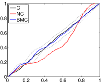
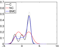
$\psi=5$

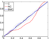
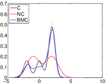
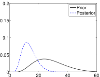
Figure 1: Infinite beta mixture calibrated (BMC), calibrated (C) and non calibrated (NC) combinations for a dataset of 1,000 samples from $p_{1}\mathcal{N}(-2,0.25)+p_{2}\mathcal{N}(0,0.25)+p_{3}\mathcal{N}(2,0.25)$ with $\bm{p}=(1/5,1/5,3/5)$. PITs cdf (left graph) and calibrated pdf (middle graph) of the combination models C (black), NC (red) and BMC (blue) and BMC 99% HPD (gray). Prior (black) and posterior (blue) number of components of the random BMC model (right graph).

The left charts of Figure 1 report the PITs of the average infinite beta mixture calibration (BMC) model and their 99% credibility intervals obtained from 1,000 MCMC samples after convergence. The PITs of the calibrated model (black lines) belong to the credibility interval of the BMC, thus the resulting predictive cdf is well calibrated. We should notice that the credibility intervals are usually larger than the one obtained using a beta mixture with a fixed number of components. In fact the calibrated density accounts for both calibration parameter uncertainty and also for the uncertainty about the number of mixture components. A comparison between the top- and bottom-right chart also shows that an increase in the value of the dispersion parameter usually increases the uncertainty.

The credibility intervals (gray lines) obtained with the infinite beta mixture calibration model, see Figure 1, always contain the PITs (first column) and the predictive density function (second column) of the correct model. The infinite BMC seems particularly accurate in the tails (last column). We also note that the uncertainty of the number components in the infinite beta mixture implies a wider high probability density region (HPD), see gray lines in 1, than that given by the finite beta mixture calibration, see third panel in 8. The prior and posterior distributions of the number of mixture components in BMC are given in the right graph in Figure 1. The posterior density is more concentrated than the prior, suggesting that data are informative on the number of calibration components.

In the second set of experiments, we assume that the data are generated by the following mixture of $t$-distributions, i.e.

$$y_{t}\overset{i.i.d.}{\sim}\frac{1}{2}\mathcal{T}(-1,1,6)+\frac{1}{2}\mathcal{T}(2,1,6),\quad t=1,\ldots,2000,$$

where $\mathcal{T}(\mu,\sigma,\nu)$ denotes a $t$-distribution with location, scale and degrees of freedom parameters $\mu$, $\sigma$ and $\nu$ respectively. The results in Supplementary Materials S4 show the difficulties of the beta model in achieving well calibrated PITs. In this set of experiments we assume $\psi$ is unknown. The results of the infinite mixture calibration are given in Figure 2.

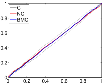
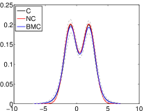
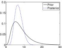
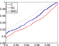
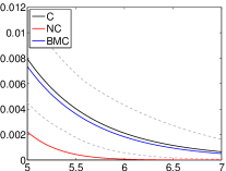
Figure 2: Infinite beta mixture calibrated (BMC), calibrated (C) and non calibrated (NC) combinations for a dataset of 2,000 samples from $1/2\mathcal{T}(-1,1,6)+1/2\mathcal{T}(2,1,6)$. PITs cdf (left graphs) and calibrated pdf (middle graphs) of the combination models C (black), NC (red) and BMC (blue) and BMC 99% HPD (gray). Prior (black) and posterior (blue) number of components of the random BMC model (right graph).

Both cdf (first column) and pdf (second column) indicate that the Bayesian BC has problems producing well-calibrated predictions. The Bayesian nonparametric calibration BMC, on the contrary, produces well-calibrated densities, in particular on the tails; see also the 99% credibility intervals. We note that the posterior distribution of the number of clusters is more concentrated than the prior, thus there is learning from the data on the number of mixture components. Finally, our experiments changing the dispersion parameter indicate no substantial changes in the posterior density over different hyperparameter values.

5.2 Dependent observations

We assume that a predictive density is obtained from the combination of two independent normal autoregressive processes of the first order, $y_{t}=\mu_{1}+\phi y_{t-1}+\varepsilon_{1t}$ and $y_{t}=\mu_{2}+\phi y_{t-1}+\varepsilon_{2t}$ with $\varepsilon_{it}\sim\mathcal{N}(0,\sigma_{i}^{2})$ i.i.d., where $\mu_{1}=-1$, $\mu_{2}=2$ and $\sigma_{1}=\sigma_{2}=0.5$. Following the notation used in Example 4.4 we assume the data generating process is a mixture of skew-normal autoregressive processes (mAR)

$$y_{t}\sim\frac{1}{3}\mathcal{S}\mathcal{N}(-2+\phi y_{t-1},0.5,\varrho)+\frac{2}{3}\mathcal{S}\mathcal{N}(2+\phi y_{t-1},0.5,\varrho),$$

$t=1,\ldots,1000$. We compare the NC and BMC combination schemes defined in the previous section. We set the BMC dispersion parameter $\psi=0.1$ and consider two settings for the autoregressive coefficients: low persistence ($\phi=0.5$, panel (a) in Figure 3) and high persistence ($\phi=0.99$, panel (b)). For the skewness parameter, we consider one of the cases covered in Example 4.4, i.e. $\varrho=-1$ (first column in panels (a) and (b)). Moreover we show, through simulated examples, that the well-calibration property is satisfied also for other two cases: $\varrho=-3$ and $\varrho=-5$ (columns two and three in panels (a) and (b)).

(a) Low persistence ($\phi=0.5$)
$\varrho=-1$	$\varrho=-3$	$\varrho=-5$
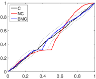
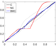
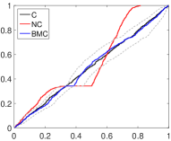
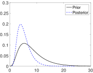
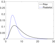
(b) High persistence ($\phi=0.99$)
$\varrho=-1$	$\varrho=-3$	$\varrho=-5$

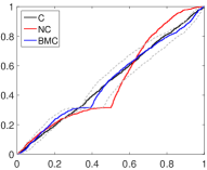
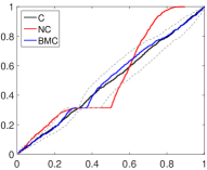
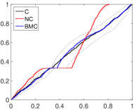
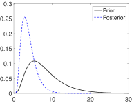
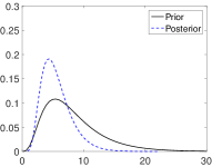
Figure 3: Infinite beta mixture calibrated (BMC), calibrated (C) and non calibrated (NC) combinations for a dataset of 1,000 samples from the autoregressive mixture model mAR. Top: PITs cdf of the combination models C (black), NC (red) and BMC (blue) and BMC 99% HPD (gray). Bottom: prior (black) and posterior (blue) number of components of the random BMC model.

6 Empirical applications

Then, we investigate relative predictability accuracy for the out-of-sample period. Precisely, as in Geweke and Amisano, (2010), Geweke and Amisano, (2011) and Kapetanios et al., (2015), we evaluate the predictive densities using the Kullback Leibler Information Criterion (KLIC) based measure, utilizing the expected difference in the Logarithmic Scores of the candidate forecast densities. The KLIC computes the distance between the true density of a random variable and some candidate density. Even though the true density is not known, for the comparison of two competing models, it is sufficient to consider the average Logarithmic Score (AvLS). The continuous ranked probability score (CRPS) at time $t$ for model $k$ is defined as:

$$\hbox{CRPS}_{t,k}=\int\left(F_{t,k}(z)-\mathbbm{1}_{[y_{t},+\infty)}(z)\right)^{2}\text{d}z$$

where $F_{t,k}(y)$ and $f_{t,k}(y)$ are the predictive cdf and pdf, respectively, for model $k$, conditional to the information available up to time $t-1$.

6.1 Stock returns

The first application considers S&P500 daily percent log returns data from 3 January 1972 to 31 December 2008, an updated version of the database used in studies such as Geweke and Amisano, (2010), Geweke and Amisano, (2011) and Kapetanios et al., (2015). We estimate a Normal GARCH(1,1) model and a $t$-GARCH(1,1) model via maximum likelihood (ML) using rolling samples of 1250 trading days (about five years) and produce one day ahead density forecasts. The first one day ahead forecast refers to December 15, 1975. The predictive densities are formed by substituting the ML estimates for the unknown parameters. We combine the two predictive densities using a linear pooling with recursive log score weights, see description in Section 5. Also in this section, we refer to it as the non-calibrated model. Furthermore we consider our mixture of beta probability density functions (BMC) to achieve better calibration properties. We split the sample in two periods. The data from December 15, 1975 to December 31, 2006 are used for an in-sample calibration of our method to investigate its properties over a long period. The data from January 3, 2007 to December 31, 2008 for a total of 504 observations, are used for our out-of-sample analysis. Therefore, we extend evidence in Geweke and Amisano, (2010) and Geweke and Amisano, (2011) by focusing on the period related to Great Financial Crisis, with the first semester of 2007 considered a tranquil period and the remaining part of the sample corresponding to the most turbulent times. In this experiment, we fit the calibration over a moving window of 250 days and produce one-day ahead forecasts.

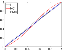
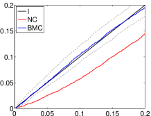
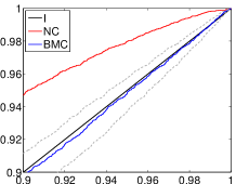
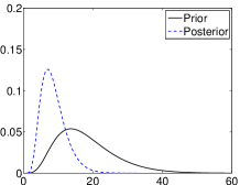
Figure 4: Infinite beta mixture calibrated (BMC), calibrated (C) and non calibrated (NC) combinations for the S&P500 daily percent log returns data. PITs cdf (lines from 1 to 3) of the idea model I C (black), combination models NC (red) and BMC (blue) and BMC 99% HPD (gray). Prior (black) and posterior (blue) number of components of the random BMC model (bottom).

First, we compare the two individual models and the two combinations in terms of calibration, measured as PIT, over the full sample period (in-sample and out-of-sample periods). Figure 4 reports calibration results for the in-sample analysis. The BMC line is the closer to the 45 degree line, which represents the PIT plot for the unknown true/ideal model. This 45 degree line always belongs to the confidence interval of the BMC. NC is not calibrated for all quantiles. In particular, on the upper and lower tails, the NC differs substantially from the BMC. As in the simulation exercises the posterior density for the numbers of beta components in BMC is more concentrated than the prior.

Table 1: Average log scores for the Normal GARCH model (Normal), $t$-GARCH model (Student-$t$), linear pooling (NC) and beta mixture calibration (BMC) over the sample period from January 1, 2007 to December 31, 2008.

	Normal	Student-$t$	NC	BMC
AvLS	-2.311	-1.650	-1.827	-1.450

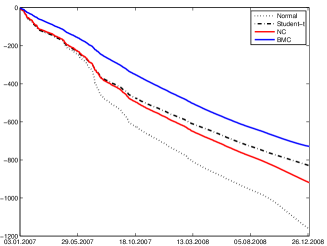
Figure 9: Cumulative log scores for the Normal GARCH model (Normal), $t$-GARCH model (Student-$t$), linear pooling (NC) and beta mixture calibration (BMC) over the sample period from January 1, 2007 to December 31, 2008.

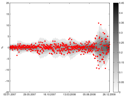
Figure 11: Fanchart of the BMC model and observations (red points) over the sample period from January 1, 2007 to December 31, 2008.

We now turn our attention to the out-of-sample analysis and the log score results. Table 1 reports average log scores for the 4 forecasting methods. BMC provides the highest score. Figure 9 in Supplementary Materials S5 shows that after the initial weeks of January 2007 where models perform similarly, BMC outperforms the other three approaches. The $t$-model provides higher scores than the normal one and the non-calibrated combination. The accuracy of the normal Garch model is very low during our OOS period, in particular on the extreme events, which results in deteriorating NC performance after August 2007, the beginning of the turbulent times. Just selecting the $t$-GARCH version or, even better, applying local weights as in our BMC improves accuracy. Figure 11 in S5 shows the BMC-based predictive density.

6.2 Wind speed

The second empirical example considers the dataset used in Lerch and Thorarinsdottir, (2013). It consists of 50 ensemble member predictions (Molteni et al.,, 1996) of wind speed at ten meters above the ground, obtained from the global ensemble prediction system of the European Centre for Medium-Range Weather Forecasts (ECMWF). We restrict our attention to the ensemble predictions for the maximum wind speed at the station at Frankfurt airport. The station ensemble forecasts are obtained by bilinear interpolation of the gridded model output.

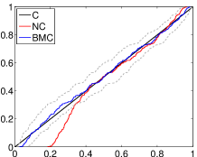
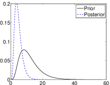
Figure 5: Infinite beta mixture calibrated (BMC), calibrated (C) and non calibrated (NC) combinations for the maximum wind speed at the station at Frankfurt airport. PITs (left top) of the combination models C (black), NC (red) and BMC (blue) and BMC 99% HPD (gray). Prior (black) and posterior (blue) number of components of the random BMC model (right top).

We consider the ECMWF ensemble run initialized at 00 hours UTC with a horizontal resolution of about 33 km, a temporal resolution of 3-6 hours and lead times of 3, 6 and 24 hours. To obtain predictions of daily maximum wind speed, we take the daily maximum of each ensemble member at the Frankfurt location. One day ahead forecasts are given by the maximum over lead times. The observations are hourly observations of 10-minute average wind speed which is measured over the 10 minutes before the hour. To obtain daily maximum wind speed, from 1 May 2010 to 30 of April 2011, we take the maximum over the 24 hours corresponding to the time frame of the ensemble forecast.

The results presented below are based on a verification period from 9 August 2010 to 30 April 2011, consisting of 263 individual forecast cases. Additionally, we use data from 1 February 2010 to 30 April 2011 to obtain training periods of equal length for all days in the verification period and for model selection purposes and forecasts from May 1, 2010 to 8 August 2010 (100 observations) as initial training period for the combination methods.

Following Lerch and Thorarinsdottir, (2013), we consider two competing models: the truncated normal distribution (TN) and the generalized extreme value distribution (GEV). The TN model is estimated by minimizing the CRPS. The GEV model is estimated by maximum likelihood estimation.

First, we report in-sample results over the sample from May 1, 2010 to 30 April 2011. Then, we implement an out-of-sample exercise for the period from August 9, 2010 to 30 April 2011. We report both log score and CRPS results.

Table 2: Average log scores (AvLS) and average CRPS (AvCRPS) for the truncated normal (TN), the generalized extreme value distribution (GEV), linear pooling (NC) and beta mixture calibration (BMC) over the sample period from August 9, 2010 to 30 April 2011.

	TN	GEV	NC	BMC
AvLS	-2.812	-2.904	-2.433	-1.997
AvCRPS	1.346	1.802	1.314	0.982

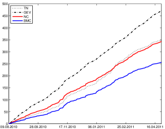
Figure 10: Cumulative CRPS for the truncated normal (TN), the the generalized extreme value distribution (GEV), linear pooling (NC) and beta mixture calibration (BMC) over the sample period from August 9, 2010 to 30 April 2011.

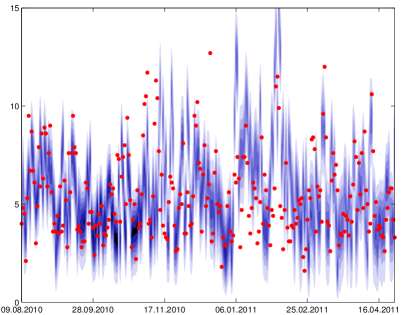
Figure 12: Fanchart of the BMC model and observations (red points) over the sample period from August 9, 2010 to 30 April 2011.

Figure 5 reports in-sample calibration results. The BMC line is close to the ideal model and always includes the 45 degree line in the confidence interval. The NC performs poorly for small quantiles. The posterior density for the numbers of beta components in BMC is more concentrated than the prior, confirming also in this exercise that data are informative on the number of mixture components. When focusing on the OOS exercise, the BMC predictive distribution predicts accurately and provides the highest average LS and the lowest average CRPS in Table 2. Gains are substantial, as Figure 10 in Supplementary Materials S5 shows. The distribution is often multimodal, see Figure 12 in Supplementary Materials S5, with the highest mode at low values of wind speed, and a second mode concentrated around values of wind speed greater than 5 meters per second. The truncated normal has too many values in the lower and upper tails; the GEV is too skewed to the upper tail, thus predicting on average too high values. The NC is also upper biased by the GEV. The BMC shifts the probability mass of the predictive distribution from the upper tail to the central part and the left tail, thus producing better calibrated forecasts.

7 Discussion

We propose a Bayesian approach to predictive density combination and calibration. We build on the predictive density calibration framework of Ranjan and Gneiting, (2010) and Gneiting and Ranjan, (2013) and propose infinite beta mixtures as prior distributions for the calibration function. We rely upon the flexibility of the infinite beta mixtures to achieve a continuous deformation of the linear density combination. Each component of the beta mixture calibrates different parts of the predictive cdf and uses component-specific combination weights. Thanks to these features, our calibration model can also be viewed as a mixture of local combination models. Furthermore, our Bayesian framework allows for including various sources of uncertainty in the predictive density.

We provide suitable sufficient conditions for weak posterior consistency of our probabilistic calibration. The results imply uniformity of the PITs in the limit, when the number of observations goes to infinity, under both assumptions of i.i.d. and Markovian observations.

We discuss finite sample properties of our methodology in simulation exercises, showing how the infinite beta components are adequate in applications with multimodal densities, skewness and heavy tails. In empirical applications to stock returns and wind speed data, our approach provides well-calibrated and accurate density forecasts.

Supplementary Materials for: ”Bayesian Nonparametric Calibration and Combination of Predictive Distributions”
by F. Bassetti, R. Casarin, F. Ravazzolo.

Appendix S1 Computational details

S1.1 Gibbs sampler for the finite beta mixture model

1. Full conditional distribution of $D$. Samples from the full conditional of $D$ given $(\bm{\theta},Y)$ are obtained by drawing sequentially over $t$, vectors $d_{t}=(d_{1t},\ldots,d_{Kt})$ from multinomial distributions with probabilities

$$\pi(d_{kt}=1|\bm{\theta},Y)\propto w_{k}b^{*}_{\mu_{k},\nu_{k}}\left(H(y_{t}|\bm{\omega}_{k})\right)h(y_{t}|\bm{\omega}_{k})$$

for $k=1,\ldots,K$.

2. Full conditional distribution of $(\bm{\mu},\bm{\nu})$. Samples from the full conditional of $(\bm{\mu},\bm{\nu})$ given $(\bm{w},\bm{\omega},D,Y)$ are obtained in a sequence of Metropolis-Hastings (MH) steps on a transformed space. Following Bouguila et al., (2006), we let: $\mu_{k}=1/(1+\exp\{-\gamma_{k}\})$ and $\nu_{k}=\exp\{\lambda_{k}\}$, $k=1,\ldots,K$ and draw iteratively from

$$\pi(\gamma_{k},\lambda_{k}|\bm{w},\bm{\omega},D,Y)\propto$$

$$\prod_{t\in\mathcal{D}_{k}}b^{*}_{\mu_{k},\nu_{k}}\left(H(y_{t}|\bm{\omega}_{k})\right)\mu_{k}^{\xi_{1\mu}-1}(1-\mu_{k})^{\xi_{2\mu}-1}\nu_{k}^{\xi_{1\nu}-1}\exp\{-\xi_{2\nu}\nu_{k}\}J(\mu_{k},\nu_{k}),$$

where $J(\mu_{k},\nu_{k})=\exp\{-\gamma_{k}-\lambda_{k}\}(1+\exp\{-\gamma_{k}\})^{-2}(1+\exp\{-\lambda_{k}\})^{-2}$ is the Jacobian of the transform. In the MH we use a Gaussian random walk proposal distribution with covariance matrix $\Sigma=0.05I_{2}$, which yields acceptance rates of about 0.4.

3. Full conditional distribution of $\bm{\omega}$. Samples from the full conditional of $\bm{\omega}$ given $(\bm{w},\bm{\mu},\bm{\nu},D,Y)$ are obtained by drawing iteratively $\bm{\omega}_{k}$, $k=1,\ldots,K$. At each step we apply a MH with the prior distribution as proposal. The acceptance probability of each MH step is:

$$\min\left\{\prod_{t\in\mathcal{D}_{k}}\frac{b^{*}_{\mu_{k},\nu_{k}}(H(y_{t}|\bm{\omega}^{*}))h(y_{t}|\bm{\omega}^{*})}{b^{*}_{\mu_{k},\nu_{k}}(H(y_{t}|\bm{\omega}_{k}))h(y_{t}|\bm{\omega}_{k})},1\right\},$$

where $\bm{\omega}^{*}\sim\mathcal{D}ir(\xi_{\omega},\ldots,\xi_{\omega})$.

4. Full conditional distribution of $\bm{w}$. Samples from the full conditional of $\bm{w}$ given $(\bm{\omega},\bm{\mu},\bm{\nu},D,Y)$ are obtained by exploiting the conjugacy of the prior distribution, in that

$$\pi(w_{1},\ldots,w_{k}|\bm{\omega},\bm{\mu},\bm{\nu},D,Y)\propto\mathcal{D}ir(\xi_{w}+T_{1},\ldots,\xi_{w}+T_{k}).$$

When $K=1$, we replace the single-move Gibbs sampler with a global MH sampler with target distribution obtained by applying to the joint posterior

$$\pi(\mu,\nu,\omega|Y)\propto\prod_{t=1}^{T}b^{*}_{\mu,\nu}\left(H(y_{t}|\omega)\right)h(y_{t}|\omega)\mu^{\xi_{1\mu}-1}(1-\mu)^{\xi_{2\mu}-1}$$

$$\times\;\nu^{\xi_{1\nu}-1}\exp\{-\xi_{2\nu}\nu\}\omega^{\xi_{1\omega}-1}(1-\omega)^{\xi_{2\omega}-1}$$

where $Y=(y_{1},\ldots,y_{t})$, the change of variable $\mu=1/(1+\exp\{-\theta_{1}\})$, $\nu=\exp\{\theta_{2}\}$ and $\omega=1/(1+\exp\{-\theta_{3}\}$. We consider a random walk proposal on the transformed parameter space accounting for the Jacobian of the transformation, that is, $J=\exp\{\theta_{2}-\theta_{1}-\theta_{3}\}(1+\exp\{-\theta_{1}\})^{-2}(1+\exp\{-\theta_{3}\})^{-2}$. Setting the covariance matrix to $\Sigma=\hbox{diag}\{0.1,0.05,0.1\}$, we achieve acceptance rates of about 0.4.

S1.2 Gibbs sampler for the infinite beta mixture model

Let $\mathcal{D}_{k}=\{t=1,\ldots,T|d_{t}=k\}$ denote the set of indexes of the observations allocated to the $k$-th component of the mixture and with $\mathcal{D}=\{k|\mathcal{D}_{k}\neq\emptyset\}$ the set of indexes of the non-empty mixture components. Then the cardinality of $\mathcal{D}$, $Card(\mathcal{D})$, gives the number of mixture components and $D^{*}=\sup\mathcal{D}$ can be interpreted as the number of stick-breaking components used in the mixture. As noted by Kalli et al., (2011), the sampling of an infinite numbers of $\Theta$ and $V$ is not necessary, since only the elements in the full conditional pdfs of $D$ are needed. The maximum number of atoms and stick-breaking components to sample is $N^{*}=\max\{t=1,\ldots,T|N^{*}_{t}\}$, where $N^{*}_{t}$ is the smallest integer such that $\sum_{j=1}^{N^{*}_{t}}w_{j}>1-u_{t}$. Thus sampling from the joint $\pi(V,U|\Theta,D,Y,\psi)$ is obtained by splitting $V=(V^{*},V^{**})$, where $V^{*}=(v_{1},\ldots,v_{D^{*}})$ and $V^{**}=(v_{D^{*}+1},\ldots,v_{N^{*}})$, and by further collapsing the Gibbs, that is by sampling from $\pi(V^{*}|\Theta,D,Y,\psi)$ and $\pi(U|V^{*},\Theta,D,Y,\psi)$ and then from $\pi(V^{**}|V^{*},U,\Theta,D,Y,\psi)$.

1. Full conditional distribution of $V^{*}$. Sampling from the full conditional of $V^{*}$ given $(D,\Theta,Y,\psi)$ is obtained by drawing $v_{k}$, with $k\leq D^{*}$, from the full conditionals

$$\pi(v_{k}|D,Y)\propto(1-v_{k})^{\psi+b_{k}-1}v_{k}^{a_{k}},$$

that is, the PDF of a $\mathcal{B}e(a_{k}+1,b_{k}+\psi)$ with $a_{k}=\sum_{t=1}^{T}\mathbbm{1}_{\{d_{t}=k\}}$ and $b_{k}=\sum_{t=1}^{T}\mathbbm{1}_{\{d_{t}>k\}}$.

2. Full conditional distribution of $U$. Samples from the full conditional of $U$ given $(V,D,\Theta,Y,\psi)$ is obtained by simulating from the uniform

$$\pi(u_{t}|V,D,Y)\propto\frac{1}{w_{d_{t}}}\mathbbm{1}_{\{u_{t}<w_{d_{t}}\}}$$

for $t=1,\ldots,T$.

3. Full conditional distribution of $V^{**}$. Sampling from the full conditional of $V^{**}$ given $(V^{*},U,D,\Theta,Y,\psi)$ is obtained by sampling from

$$\pi(v_{k}|U,D,Y)\propto(1-v_{k})^{\psi-1},$$

that is, the PDF of a $\mathcal{B}e(1,\psi)$, with $k=D^{*}+1,\ldots,N^{*}$.

4. Full conditional distribution of $\Theta$. Sample the elements $k$, $k=1,\ldots,N^{*}$, of $\Theta$ given $(U,D,V,Y,\psi)$, from the full conditional

$$\!\!\!\!\!\!\!\!\!\pi(\bm{\theta}_{k}|U,D,V,Y)\propto\prod_{t\in\mathcal{D}_{k}}\!\!b^{*}_{\mu_{k},\nu_{k}}\!\!\left(H(y_{t}|\bm{\omega}_{k})\right)h(y_{t}|\bm{\omega}_{k})$$

$$\times\;\mu_{k}^{\xi_{\mu}-1}(1-\mu_{k})^{\xi_{\mu}-1}\nu_{k}^{\xi_{\nu}/2}\exp\{-\xi_{\nu}\nu_{k}/2\}\prod_{i=1}^{M}\omega_{ik}^{\xi_{\omega}-1}\mathbbm{1}_{\{\bm{\omega}_{k}\in\Delta_{M}\}}$$

for $k\in\mathcal{D}$, and from the prior $G_{0}$ for $k\notin\mathcal{D}$. We sample from the full conditional by iterating over the following steps:

1. $\pi(\mu_{k},\nu_{k}|\bm{\omega}_{k},U,D,V,Y,\psi)$

2. $\pi(\bm{\omega}_{k}|\mu_{k},\nu_{k},U,D,V,Y,\psi)$.

We apply here the same sampling strategy described for the parameter of the finite beta mixture model.

5. Full conditional distribution of $D$. Samples from the full conditional of $D$ given $(V,U,\Theta,Y,\psi)$ are obtained by sampling from

$$\pi(d_{t}|V,U,Y)\propto\mathbbm{1}_{\{u_{t}<w_{d_{t}}\}}f_{\mu_{d_{t}},\nu_{d_{t}}}\left(H(y_{t}|\bm{\omega}_{d_{t}})\right)h(y_{t}|\bm{\omega}_{d_{t}}),$$

with $d_{t}\in\{1,\ldots,N_{t}^{*}\}$, where $N_{t}^{*}$ is defined above.

6. Full conditional distribution of $\psi$. If the dispersion parameter $\psi$ is assumed to be random with $\mathcal{G}a(c,d)$ prior, then an extra step is needed in the Gibbs sampler. More specifically, the full conditional distribution of $\psi$ given $U$, $D$, $V$ and $\Theta$ has density

$$\pi(\psi|K,T)\propto B(\psi,T)\psi^{K+c-1}\exp\{-d\psi\}\mathbbm{1}_{\psi\in(0,+\infty)},$$

which depends only on the number of observations $T$ and the number of mixture components $N^{*}$, which has been defined above.

The Gibbs sampler can used to generate draws from the predictive distribution $\hat{F}_{T+1}(y_{T+1})$. At each iteration a uniform random variable $u^{(i)}$ is sampled from the unit interval and $\bm{\theta}_{j}^{(i)}$ is used such that $w_{j-1}^{(i)}<u^{(i)}<w_{j}^{(i)}$. If $j>N^{*\,(i)}$, then more weights are required than currently exist, and they can be sampled from $\mathcal{B}e(1,\psi)$ and the additional $\bm{\theta}_{j}^{(i)}$ from $G_{0}$. Having taken $\bm{\theta}_{j}^{(i)}$, $y_{T+1}^{(i)}$ can be sampled from $B^{*}_{\mu_{j}^{(i)},\nu_{j}^{(i)}}\left(H(y_{T+1}|\bm{\omega}_{j}^{(}i))\right)$.

Appendix S2 Calibration consistency

If the pooling parameters are fixed, say $\bm{\omega}=\bm{\omega}_{0}$, the inference is necessarily limited to the calibration parameters $\bm{\theta}_{c}=(\mu,\nu)$, hence $\Theta=[0,1]\times\mathbb{R}^{+}$ and $G$ is a DP process on $\mathcal{M}([0,1]\times\mathbb{R}^{+})$ with base measure $G_{0}$ and (known) concentration parameter $\psi$.

In this special case $\Pi^{*}$ turns out to be the prior induced by

$$G\mapsto\int b^{*}_{\bm{\theta}_{c}}(H(y|\bm{\omega_{0}}))G(d\bm{\theta}_{c})h(y|\bm{\omega_{0}})$$

when $G\sim DP(\psi,G_{0})$. Then, the analogous of Theorem 4.1 is given below.

Theorem S2.1.

Let $\bm{\omega_{0}}$ be a given point in $\Delta_{M}$ such that $h(\cdot|\bm{\omega_{0}})$ is continuous and for every compact set $C\subset\mathcal{Y}$,

$$\inf_{y\in C}h(y|\bm{\omega_{0}})>0.$$ (S18)

Assume that $f_{0}$ is a continuous density on $\mathcal{Y}$ such that (15) holds with $\bm{\omega_{0}}$ in place of $\bm{\omega^{*}}$. If $G_{0}$ has full support, then $f_{0}\in KL(\Pi^{*})$.

In the previous theorem, contrary to Theorem 4.1, $\bm{\omega_{0}}$ represents the true parameter. We do not assume $\bm{\omega_{0}}$ is in the interior of $\Delta_{M}$, which means that the set of models in the combination scheme can be complete. In some situations, it is useful to consider a base measure $G_{0}$ without full support. In this spirit, following the techniques of Tang et al., (2007), we can prove the next result.

Theorem S2.2.

Let $\bm{\omega_{0}}$ be a given point in $\Delta_{M}$ and let

$$f_{0}(y)=u_{0}(H(y|\bm{\omega_{0}}))h(y|\bm{\omega_{0}})$$

with $u_{0}(x)=w_{0}b_{\mu_{0},\nu_{0}}^{*}(x)+(1-w_{0})\int_{(0,1)\times\mathbb{R}^{+}}b_{\mu,\nu}^{*}(x)P_{0}(d\mu d\nu)$, $P_{0}$ being a probability measure on $(0,1)\times\mathbb{R}^{+}$. If $(\mu_{0},\nu_{0})$ belong to $supp(G_{0})$, $\text{supp}(P_{0})\subset\text{supp}(G_{0})$, and for some $\zeta>0$ and $0<\eta<\min(\mu_{0},1-\mu_{0},\nu_{0},w_{0})$ one has

$$\int_{0}^{1}\frac{u_{0}(x)^{\zeta+1}}{x^{\zeta A}(1-x)^{\zeta B}}dx<+\infty,$$ (S19)

for $A=(\mu_{0}+\eta)(\nu_{0}+\eta)-1$ and $B=(1-\mu_{0}+\eta)(\nu_{0}+\eta)-1$, then $f_{0}\in KL(\Pi^{*})$.

We shall notice that the specification of the calibration function $u_{0}$ in the true density $f_{0}$ can be used to build a statistical procedure for testing the hypothesis of well calibrated PITs against the alternative of not well-calibrated PITs.

Appendix S3 Proofs

S3.1 Proofs of the results of Sections 4.1 and S2

The proof of Theorem 4.1 is based on an application of Theorem 1 and Lemma 3 of Wu and Ghosal, 2009a ; Wu and Ghosal, 2009b . For the shake of clarity we report the statements of these results in Theorems S3.1 below.

Theorem S3.1 (Theorem 1 and Lemma 3 of Wu and Ghosal, 2009a ).

Let $\Theta$ be a separable metric space. If for any $\epsilon>0$ there is a probability measure $G_{\epsilon}\in supp(\Pi)$ and a closed set $D_{\epsilon}$ such that

• $\int\log(f_{0}/f_{G_{\epsilon}})f_{0}<\epsilon$,

• $D_{\epsilon}$ contains $\sup(G_{\epsilon})$ in its interior and

  $$\int\log\Big{(}\frac{f_{G_{\epsilon}}(y)}{\inf_{\theta\in D_{\epsilon}}K(y;\theta)}\Big{)}f_{0}(y)dy<+\infty,$$

• $\inf_{y\in C}\inf_{\theta\in D_{\epsilon}}K(y;\theta)>0$ for every compact set $C\subset\mathcal{Y}$,

• $\{\theta\mapsto K(y;\theta):y\in C\}$ is uniformly equicontinuous on $D_{\epsilon}$,

then $f_{0}\in KL(\Pi^{*})$.

Assumption (H1) corresponds to (A1) in Theorem 1 of Wu and Ghosal, 2009a . Assumptions (H2)-(H3) correspond to assumptions (A7)-(A8) of Lemma 3 of Wu and Ghosal, 2009a , while (H5) is slightly different from the original assumption (A9), see Wu and Ghosal, 2009b . In order to apply the results given above, it is useful to reformulate Theorem 4.1 as follows.

Theorem S3.2.

Assume that the functions $f_{m}(\cdot)$ are continuous on $\mathcal{Y}$. Let $u_{0}$ be a continuous density on $(0,1)$ such that

$$\begin{split}&\int_{0}^{1}[|\log(x)|+|\log(1-x)|]u_{0}(x)dx<+\infty\\ &\text{and}\quad\int_{0}^{1}\log(u_{0}(x))u_{0}(x)dx<+\infty.\\ \end{split}$$ (S20)

Let $f_{0}(y)=u_{0}(H(y|\bm{\omega^{*}}))h(y|\bm{\omega^{*}})$ with $\bm{\omega^{*}}$ in the interior of $\Delta_{M}$ and assume that, for every compact set $C\subset\mathcal{Y}$,

$$\inf_{y\in C}h(y|\bm{\omega^{*}})>0.$$ (S21)

Then $f_{0}\in KL(\Pi^{*})$ whenever $G_{0}$ has full support.

Proof of Theorem S3.2.

Here we need to think $\Delta_{M}$ as the set $\{(\omega_{1},\dots,\omega_{M-1})\in[0,1]^{M-1}:\sum_{i=1}^{M-1}\omega_{i}\leq 1\}$ endowed with the topology induced by the euclidean norm. Clearly, $\omega_{M}$ will denote $1-\sum_{i=1}^{M-1}\omega_{i}$.

Verification of H1 of Theorem S3.1. Since $u_{0}$ is continuous on $(0,1)$ and $\int_{0}^{1}\log(u_{0}(x))u_{0}(x)dx<+\infty$ by Theorem 1 in Robert and Rousseau, (2002) there is

$$u_{\epsilon}(x)=u_{\tilde{P}_{\epsilon}}(x)=\sum_{i=1}^{K_{\epsilon}}w_{i,\epsilon}b^{*}_{\mu_{i,\epsilon},\nu_{i,\epsilon}}(x),$$

where $\tilde{P}_{\epsilon}(d\mu d\nu):=\sum_{i=1}^{K_{\epsilon}}w_{i,\epsilon}\delta_{\mu_{i,\epsilon},\nu_{i,\epsilon}}(d\mu d\nu)$, such that $KL(u_{0},u_{\epsilon})\leq\epsilon$. If $G_{\epsilon}(d\bm{\omega}d\mu d\nu):=\delta_{\bm{\omega^{*}}}(d\bm{\omega})\times\tilde{P}_{\epsilon}(d\mu d\nu)$, then

$$f_{G_{\epsilon}}(y)=\int b^{*}_{\mu,\nu}(H(y|\bm{\omega}))h(y|\bm{\omega})G_{\epsilon}(d\bm{\omega}d\mu d\nu)=u_{\epsilon}(H(y|\bm{\omega^{*}}))h(y|\bm{\omega^{*}}).$$

By a simple change of variables,

$$\begin{split}KL(f_{0},f_{G_{\epsilon}})&=\int u_{0}(H(y|\bm{\omega^{*}}))h(y|\bm{\omega^{*}})\log\Big{(}\frac{u_{0}(H(y|\bm{\omega^{*}}))h(y|\bm{\omega^{*}})}{u_{\epsilon}(H(y|\bm{\omega^{*}}))h(y|\bm{\omega^{*}})}\Big{)}dy\\ &=\int_{0}^{1}u_{0}(z)\log\Big{(}\frac{u_{0}(z)}{u_{\epsilon}(z)}\Big{)}dz.\\ \end{split}$$

That is

$$KL(f_{0},f_{G_{\epsilon}})=KL(u_{0},u_{\epsilon})\leq\epsilon.$$

Note that $supp(G_{\epsilon})=\{\bm{\omega^{*}}\}\times\cup_{i=1}^{K_{\epsilon}}\{(\mu_{i,\epsilon},\nu_{i,\epsilon})\}$ and, since $G_{0}$ has full support, $G_{\epsilon}\subset supp(Dir(\psi,G_{0}))$.

Verification of H2 of Theorem S3.1. One can find a compact set $D_{\epsilon}^{*}$ in $(0,1)\times(0,+\infty)$ such that $D_{\epsilon}^{*}$ contains $\cup_{i=1}^{K_{\epsilon}}\{(\mu_{i,\epsilon},\nu_{i,\epsilon})\}$ in its interior. Moreover, recalling that $h(y|\bm{\omega})=\sum_{i=1}^{M}\bm{\omega}_{i}f_{i}(y)$ and that $\bm{\omega^{*}}$ is in the interior of $\Delta_{M}$, one can find a (sufficiently small) compact set $\Delta_{\epsilon}^{*}\subset\Delta_{M}$ containing $\bm{\omega^{*}}$ in its interior such that if $\bm{\omega}\in\Delta_{\epsilon}^{*}$ then $C_{1,\epsilon}h(y|\bm{\omega^{*}})\leq h(y|\bm{\omega})\leq C_{2,\epsilon}h(y|\bm{\omega^{*}})$ for every $y$. It follows that $D_{\epsilon}=\Delta_{\epsilon}^{*}\times D_{\epsilon}^{*}$ is a compact set containing $supp(G_{\epsilon})$ in its interior. Noticing that if $\bm{\omega}\in\Delta_{\epsilon}^{*}$ then $C_{2,\epsilon}H(y|\bm{\omega^{*}})\geq H(y|\bm{\omega})\geq C_{1,\epsilon}H(y|\bm{\omega^{*}})$ and $C_{2,\epsilon}(1-H(y|\bm{\omega^{*}}))\geq(1-H(y|\bm{\omega}))\geq C_{1,\epsilon}(1-H(y|\bm{\omega^{*}}))$, one can write

$$\begin{split}I_{\epsilon}(y)&:=\inf_{(\bm{\omega},\mu,\nu)\in D_{\epsilon}}K(y;\bm{\omega},\mu,\nu)\\ &=\inf_{(\bm{\omega},\mu,\nu)\in D_{\epsilon}}h(y|\bm{\omega})\frac{H(y|\bm{\omega})^{\mu\nu-1}(1-H(y|\bm{\omega}))^{(1-\mu)\nu-1}}{B(\mu\nu,(1-\mu)\nu)}\\ &\geq C_{3,\epsilon}h(y|\bm{\omega^{*}})H(y|\bm{\omega^{*}})^{A_{\epsilon}-1}(1-H(y|\bm{\omega^{*}}))^{B_{\epsilon}-1}=:I^{*}_{\epsilon}(y)\\ \end{split}$$

where $C_{3,\epsilon}=C_{1,\epsilon}C_{2,\epsilon}^{-2}\inf\{C_{1,\epsilon}^{\mu\nu+(1-\mu)\nu}/B(\mu\nu,(1-\mu)\nu):(\mu,\nu)\in D_{\epsilon}^{*}\}>0$, $A_{\epsilon}=\sup\{\mu\nu:(\mu,\nu)\in D_{\epsilon}^{*}\}>0$ and $B_{\epsilon}=\sup\{(1-\mu)\nu:(\mu,\nu)\in D_{\epsilon}^{*}\}>0$. Hence, one the one hand $f_{G_{\epsilon}}(y)\geq I_{\epsilon}(y)$ and hence $\log({f_{G_{\epsilon}}(y)}/I_{\epsilon}(y))\geq 0$, on the other hand

$$\begin{split}\int\log\Big{(}\frac{f_{G_{\epsilon}}(y)}{I_{\epsilon}(y)}\Big{)}f_{0}(y)dy&\leq\int\log\Big{(}\frac{f_{G_{\epsilon}}(y)}{I^{*}_{\epsilon}(y)}\Big{)}f_{0}(y)dy\\ &\leq\int_{0}^{1}\log\Big{(}\frac{u_{\epsilon}(x)}{x^{A_{\epsilon}-1}(1-x)^{B_{\epsilon}-1}}\Big{)}u_{0}(x)dx+|\log(C_{3,\epsilon})|.\\ \end{split}$$

Since $C_{4,\epsilon}x^{A_{\epsilon}^{\prime}-1}(1-x)^{B_{\epsilon}^{\prime}-1}\leq u_{\epsilon}(x)\leq C_{5,\epsilon}x^{A_{\epsilon}^{\prime\prime}-1}(1-x)^{B_{\epsilon}^{\prime\prime}-1}$ for suitable constants, it follows that

$$\int\Big{|}\log\Big{(}\frac{u_{\epsilon}(x)}{x^{A_{\epsilon}-1}(1-x)^{B_{\epsilon}-1}}\Big{)}\Big{|}u_{0}(x)dx\leq C_{6,\epsilon}\int[|\log(x)|+|\log(1-x)|]u_{0}(x)dx<+\infty$$

by assumption (S20). Hence

$$0<\int\log\Big{(}\frac{f_{G_{\epsilon}}(y)}{\inf_{(\bm{\omega},\mu,\nu)\in D_{\epsilon}}K(y;\bm{\omega},\mu,\nu)}\Big{)}f_{0}(y)dy<+\infty.$$

Verification of H3 of Theorem S3.1. It follows immediately that, for every compact set $C$,

$$\inf_{y\in C}\inf_{(\bm{\omega},\mu,\nu)\in D_{\epsilon}}K(y;\bm{\omega},\mu,\nu)\geq\inf_{y\in C}I^{*}_{\epsilon}(y)$$

and the right hand side is strictly positive by (S21).

Verification of H4 of Theorem S3.1. The function $(\bm{\omega},\mu,\nu,y)\mapsto K(y;\bm{\omega},\mu,\nu)$ is continuous and hence uniformly continuous on the compact set $C\times D_{\epsilon}$. It follows that the family $\{(\bm{\omega},\mu,\nu)\mapsto K(y;\bm{\omega},\mu,\nu):y\in C\}$ is uniformly equicontinuous on $D_{\epsilon}$. ∎

Proof of Theorem 4.1.

Write $H_{0}$ and $h_{0}$ for $H(\cdot|\bm{\omega^{*}})$ and its density. By assumptions one gets that $H_{0}$ is continuous and strictly increasing. Hence, if one defines

$$u_{0}(x):=\frac{f(H_{0}^{-1}(x))}{h_{0}(H_{0}^{-1}(x))},$$

it follows that $f_{0}(y)=u_{0}(H_{0}(y))h_{0}(y)$. Note that $u_{0}$ turns out to be a continuous function on $(0,1)$. It remains to check that assumption (15) yields (S20). Now, a change of variable gives

$$\int|\log(H(y|\bm{\omega^{*}}))|f_{0}(y)dy=\int|\log(H(y|\bm{\omega^{*}}))|u_{0}(H_{0}(y))h_{0}(y)dy=\int|\log(x)|u_{0}(x)dx.$$

Similarly for $\int|\log(1-H(y|\bm{\omega^{*}}))|]f_{0}(y)dy$. Finally

$$KL(f_{0},h(\cdot|\bm{\omega^{*}}))=\int\log(u_{0}(H_{0}(y))u_{0}(H_{0}(y))h_{0}(y)dy=\int u_{0}(x)\log(u_{0}(x))dx.$$

∎

Proof of Theorem S2.1.

The proof is a simple modification of the proof of Theorem S3.2. ∎

Proof of Theorem S2.2.

Given any measure $Q$ on $(0,1)\times\mathbb{R}^{+}$ recall that $f_{Q}(x)=u_{Q}(H(y|\bm{\omega_{0}}))h(y|\bm{\omega_{0}})$ where $u_{Q}(x)=\int b_{\mu,\nu}^{*}(x)Q(d\mu d\nu)$. Again, by a simple change of variables, $KL(f_{G},f_{0})=KL(u_{G},u_{0})$. Hence to prove that $f_{0}\in KL(\Pi^{*})$ it suffices to prove that for every $\epsilon>0$, $P\{KL(u_{G},u_{0})\leq\epsilon\}>0$.

Now recall that if $G\sim DP(\psi,G_{0})$ then $G$ admits the representation $G=w_{1}\delta_{\theta_{1}}+(1-w_{1})G_{1}$ where $w_{1},\theta_{1}=(\mu_{1},\nu_{1})$ and $G_{1}$ are stochastically independent, $G_{1}\sim DP(\psi,G_{0})$, $w_{1}\sim Beta(1,\phi_{1})$ and $\theta_{1}\sim G_{0}$.

Given $\eta,\eta^{\prime}>0$ define $\mathcal{U}_{\eta}:=\{(w,\mu,\nu)\in(0,1)^{2}\times\mathbb{R}^{+}:|w-w_{0}|\leq\eta,|\mu-\mu_{0}|\leq\eta,|\nu-\nu_{0}|\leq\eta\}$ and $\mathcal{U}_{\eta,\eta^{\prime}}^{*}:=\{G=w_{1}\delta_{\theta_{1}}+(1-w_{1})G_{1}:(w_{1},\theta_{1})\in\mathcal{U}_{\eta},|u_{G_{1}}-u_{P_{0}}|_{1}\leq\eta^{\prime}\}$, where we denote by $|u_{1}-u_{2}|_{1}=\int|u_{1}-u_{2}|dx$ be the $L_{1}$ distance between two densities $u_{1}$ and $u_{2}$.

Note that if $G\in\mathcal{U}_{\eta,\eta^{\prime}}^{*}$ then

$$u_{G}(x)\geq w_{1}b_{\mu_{1},\nu_{1}}^{*}(x)\geq c_{\eta}x^{A_{\eta}}(1-x)^{B_{\eta}}$$

where

$$\begin{split}&c_{\eta}:=\frac{w_{0}-\eta}{B((\mu_{0}-\eta)(\nu_{0}-\eta),(1-\mu_{0}-\eta)(\nu_{0}-\eta))},\\ &A_{\eta}:=(\mu_{0}+\eta)(\nu_{0}+\eta)-1,\qquad B_{\eta}:=(1-\mu_{0}+\eta)(\nu_{0}+\eta)-1,\\ \end{split}$$

provided that $\mu_{0}-\eta,1-\mu_{0}-\eta,\nu_{0}-\eta,w_{0}-\eta$ are positive. Hence, for any $\zeta>0$,

$$\Big{[}\frac{u_{0}(x)}{u_{G}(x)}\Big{]}^{\zeta}\leq c_{\eta,\zeta}^{*}\frac{u_{0}(x)^{\zeta}}{x^{A_{\eta}\zeta}(1-x)^{B_{\eta}\zeta}}=:g^{*}(x)$$

for a suitable constant $c_{\eta,\zeta}^{*}$. By assumption (S19), there is $\zeta$ such that $C_{0}:=\int g^{*}(x)u_{0}(x)dx<+\infty$. Hence for such $(\eta,\zeta)$, by Lemma 7 of Ghosal and van der Vaart, (2007),

$$KL(u_{0},u_{G})\leq C_{1}d_{H}^{2}(u_{G},u_{0})[1+\max(0,\log(d_{H}^{-1}(u_{G},u_{0})))]$$

where $d_{H}(u_{G},u_{0})=(\int(\sqrt{u_{G}}-\sqrt{u_{0}})^{2}dx)^{1/2}$ is the Hellinger distance between $u_{0}$ and $u_{G}$. Note that the constant $C_{1}$ depends on $C_{0},\eta$ and $\zeta$ only. Since $d_{H}(u_{G},u_{0})^{2}\leq|u_{G}-u_{0}|_{1}$ (see, e.g., Corollary 1.2.1 in Ghosh and Ramamoorthi, (2003)) it follows that

$$KL(u_{0},u_{G})\leq C_{2}|u_{G}-u_{0}|_{1}^{1/2}$$

for every $G\in\mathcal{U}_{\eta,\eta^{\prime}}^{*}$ when $\eta^{\prime}$ is small enough. Now, it is easy to check that

$$|u_{G}-u_{0}|_{1}\leq 2|w_{1}-w_{0}|+|u_{\delta_{\theta_{1}}}-u_{\delta_{\theta_{0}}}|_{1}+|u_{G_{1}}-u_{P_{0}}|_{1}$$

and that $|u_{\delta_{\theta_{1}}}-u_{\delta_{\theta_{0}}}|_{1}$ goes to zero as $|\theta_{1}-\theta_{0}|\to 0$. Since if $\eta^{\prime\prime}\leq\eta$ then $\mathcal{U}_{\eta^{\prime\prime},\eta^{\prime}}^{*}\subset\mathcal{U}_{\eta,\eta^{\prime}}^{*}$, using the previous results, for every $\epsilon>0$, one can find sufficiently small $\eta^{\prime}$ and $\eta^{\prime\prime}\leq\eta$ such that if $G\in\mathcal{U}_{\eta^{\prime\prime},\eta^{\prime}}^{*}$ then $KL(u_{G},u_{0})\leq\epsilon$. By standard argument (see e.g. the proof of Thm.2 in Tang et al., (2007)) if $G_{1}$ is in a sufficiently small weak neighbourhood $V_{\eta^{\prime}}$ of $P_{0}$ then $|u_{P_{0}}-u_{G_{1}}|_{1}\leq\eta^{\prime}$, hence

$$\{G=w_{1}\delta_{\theta_{1}}+(1-w_{1})G_{1}:G_{1}\in V_{\eta^{\prime}},(w_{1},\theta_{1})\in\mathcal{U}_{\eta^{\prime\prime}}\}\subset\mathcal{U}_{\eta^{\prime\prime},\eta^{\prime}}^{*}\subset\{KL(u_{G},u_{0})\leq\epsilon\}.$$

Moreover, $supp(P_{0})\subset supp(G_{0})$ yields that $P_{0}$ belongs to the support of $Dir(\phi,G_{0})$ and hence $P(G_{1}\in V_{\eta^{\prime}})>0$, while the fact that $\theta_{1}\in supp(G_{0})$ yields that $P((w_{1},\theta_{1})\in\mathcal{U}_{\eta^{\prime\prime}})>0$. Using the independence of $(w_{1},\theta_{1})$ and $G_{1}$, one concludes

$$P(KL(u_{0},u_{G})\leq\epsilon)\geq P(G\in\mathcal{U}_{\eta^{\prime\prime},\eta^{\prime}}^{*})\geq P(G_{1}\in V_{\eta^{\prime}})P((w_{1},\theta_{1})\in\mathcal{U}_{\eta^{\prime\prime}})>0.$$

∎

S3.2 Proofs of the results of Section 4.2

As for the proof of the results for Markovian observations, the starting point is a suitable adaptation of Theorem 1 and Lemma 3 of Wu and Ghosal, 2009a . In the Markovian setting, the prior $\Pi^{*}$ on $\mathcal{F}$ is induced via the map $G\mapsto f_{G}(y|x):=\int_{\Theta}K(y|x,\bm{\theta})G(d\bm{\theta})$, where $\Theta$ is the mixing parameter space, $K(y|x,\bm{\theta})$ is a transition kernel and $G$ has a prior $\Pi$ on the space $\mathcal{M}(\Theta)$ of probability measures on $\Theta$. Recall that in our model $\Theta=\Delta_{M}\times\Theta_{1}$, where $\Delta_{M}$ and $\Theta_{1}=(0,1)\times\mathbb{R}^{+}$ are the combination and calibration parameter spaces, respectively.

Theorem S3.3.

Let $\Theta=\Delta_{M}\times\Theta_{1}$, $\Theta_{1}$ being a separable metric space. If for any $\epsilon>0$ there is a probability measure $G_{\epsilon}\in supp(\Pi)$ such that

• $\int\int\log(f_{0}(y|x)/f_{G_{\epsilon}}(y|x))f_{0}(y|x)dy\pi(dx)<\epsilon$,

• there is a closed set $D^{*}_{\epsilon}$ which contains $\sup(G_{\epsilon})$ in its interior or $D_{\epsilon}^{*}=\Delta_{M}\times D_{\epsilon}$ with $D_{\epsilon}$ is closed in $\Theta_{1}$ and $\sup(G_{\epsilon})\subset\Delta_{M}\times D_{\epsilon}^{\circ}$ ($D_{\epsilon}^{\circ}$ being the interior of $D_{\epsilon}$), for which

  $$\int\int\log\Big{(}\frac{f_{G_{\epsilon}}(y|x)}{\inf_{\theta\in D_{\epsilon}^{*}}K(y|x,\theta)}\Big{)}f_{0}(y|x)dy\pi(dx)<+\infty,$$

• $\inf_{(x,y)\in C}\inf_{\theta\in D_{\epsilon}^{*}}K(y|x,\theta)>0$ for every compact set $C\subset\mathcal{Y}\times\mathcal{Y}$,

• $\{\theta\mapsto K(y|x,\theta):(x,y)\in C\}$ is uniformly equicontinuous on $D_{\epsilon}^{*}$,

then $f_{0}\in KL(\Pi^{*})$.

Proof.

The proof follows the same lines of the proofs of Theorem 1 and Lemma 3 of Wu and Ghosal, 2009a . ∎

Theorem S3.4.

Under the assumption of Theorem 4.2 then $f_{0}\in KL(\Pi^{*})$.

Proof.

We apply Theorem S3.3 with $\Theta_{1}=(0,1)\times\mathbb{R}^{+}$, $K(y|x,\bm{\theta})=b^{*}_{\mu,\nu}(H(y|x,\bm{\omega}))h(y|x,\bm{\omega})$ with $\bm{\theta}=(\bm{\theta}_{p},\bm{\theta}_{c})$ and $G_{\epsilon}(d\bm{\omega}d\mu d\nu):=G^{*}(d\bm{\omega}d\mu d\nu)$. In this case, since $f_{G_{\epsilon}}=f_{G^{*}}=f_{0}$, M1 is automatically satisfied, so it remains to check the other assumptions.

Verification of M2 of Theorem S3.3. One can find a compact set $D_{\epsilon}$ in $(0,1)\times(0,+\infty)$ such that the support of $G_{0}$ is contained in $\Delta_{M}\times D_{\epsilon}^{\circ}$. At this stage one can check that

$$\inf_{(\mu,\nu)\in D_{\epsilon}}H(y|x,\bm{\omega})^{\mu\nu}(1-H(y|x,\bm{\omega}))^{(1-\mu)\nu}\geq H(y|x,\bm{\omega})^{A}(1-H(y|x,\bm{\omega}))^{A}\geq R_{-}(y|x)^{A}$$

where $A:=\max\{\sup\{\mu\nu:(\mu,\nu)\in D_{\epsilon}\},\sup\{(1-\mu)\nu:(\mu,\nu)\in D_{\epsilon}\}\}>0$. Hence, setting $D_{\epsilon}^{*}:=\Delta_{M}\times D_{\epsilon}$,

$$I(y|x):=\inf_{(\bm{\omega},\mu,\nu)\in D_{\epsilon}^{*}}K(y|x,\bm{\omega},\mu,\nu)\geq\frac{C_{1}r_{-}(y|x)R_{-}(y|x)^{A}}{R_{+}(y|x)}=:I^{*}(y|x)$$

where $C_{1}=\inf\{1/B(\mu\nu,(1-\mu)\nu):(\mu,\nu)\in D_{\epsilon}\}>0$. Clearly $f_{G_{\epsilon}}(y|x)\geq I(y|x)$ and hence $\log({f_{G_{\epsilon}}(y|x)}/I_{\epsilon}(y|x))\geq 0$, moreover, recalling that $f_{G_{\epsilon}}(y|x)=f_{0}(y|x)$, one can write

$$\begin{split}\int\log&\Big{(}\frac{f_{G_{\epsilon}}(y|x)}{I(y|x)}\Big{)}f_{0}(y|x)dy\leq\int\log\Big{(}\frac{f_{0}(y|x)}{I^{*}(y|x)}\Big{)}f_{0}(y|x)dy\\ &\leq\int|\log(f_{0}(y|x))|f_{0}(y|x)dy+\int|\log(I^{*}(y|x))|f_{0}(y|x)dy.\\ \end{split}$$

Combining this with the assumptions, one gets

$$0<\int\int\log\Big{(}\frac{f_{G_{\epsilon}}(y|x)}{\inf_{(\bm{\omega},\mu,\nu)\in D_{\epsilon}}K(y|x,\bm{\omega},\mu,\nu)}\Big{)}f_{0}(y|x)dy\pi(dx)<+\infty.$$

Verification of M3 of Theorem S3.3. Using the positivity assumption of the densities $h_{m}$, it follows immediately that, for every compact set $C$, $\inf_{(x,y)\in C}\inf_{(\bm{\omega},\mu,\nu)\in D_{\epsilon}}K(y|x,\bm{\omega},\mu,\nu)>0$.

Verification of M4 of Theorem S3.3. The function $(\bm{\omega},\mu,\nu,x,y)\mapsto K(y|x,\bm{\omega},\mu,\nu)$ is continuous and hence uniformly continuous on the compact set $C\times D_{\epsilon}$. It follows that the family $\{(\bm{\omega},\mu,\nu)\mapsto K(y;\bm{\omega},\mu,\nu):(x,y)\in C\}$ is uniformly equicontinuous on $D_{\epsilon}$. ∎

Proof of Theorem 4.2.

Let $A:\{f:\int|\int g(y)[f(y|x)-f_{0}(y|x)]dy|\lambda(dx)>\epsilon\}$ where $g$ is a bounded continuous function, say $|g(y)|\leq 1$. Let $C\subset\mathcal{Y}$ a compact set such that $\lambda(C^{c})<\epsilon/4$ and set $M=2\lambda(C)$. If $f\in A$ then $\int_{C}|\int g(y)[f(y|x)-f_{0}(y|x)]dy|\lambda(dx)>\epsilon/2$ and $\sup_{x\in C}\int g(y)[f(y|x)-f_{0}(y|x)]dy>\epsilon/M$. Let $x_{f}=argmax\{\int g(y)[f(y|x)-f_{0}(y|x)]dy:x\in C\}$, then if $x\in C$

$$\Big{|}\int g(y)[f(y|x)-f_{0}(y|x)]dy\Big{|}>\frac{\epsilon}{M}-R(f,x)$$

where $R(f,x):=\Big{|}\int g(y)[f(y|x)-f(y|x_{f})]dy\Big{|}+\Big{|}\int g(y)[f_{0}(y|x)-f_{0}(y|x_{f})]dy\Big{|}$. Now for every compact set $K\subset(0,1)\times\mathbb{R}^{+}$ and every compact set $C^{\prime}\subset\mathcal{Y}$ the functions $K\times C\times C^{\prime}\times\Delta_{M}\ni(\mu,\nu,x,y,\bm{\omega})\mapsto b_{\mu,\nu}^{*}(H(y|x,\bm{\omega}))$ and $C\times C^{\prime}\times\Delta_{M}\ni(x,y,\bm{\omega})\mapsto h(y|x,\bm{\omega})$ are uniformly continuous. Hence for every $\epsilon^{\prime}$ there is $\delta=\delta(\epsilon,K,C,C^{\prime})$ such that

$$\begin{split}&\sup_{(\mu,\nu,y,\bm{\omega})\in K\times C^{\prime}\times\Delta_{M}}|b_{\mu,\nu}^{*}(H(y|x,\bm{\omega}))-b_{\mu,\nu}^{*}(H(y|x^{\prime},\bm{\omega}))|\leq\epsilon^{\prime},\\ &\sup_{(y,\bm{\omega})\in C^{\prime}\times\Delta_{M}}|h(y|x,\bm{\omega})-h(y|x^{\prime},\bm{\omega})|\leq\epsilon^{\prime}\\ \end{split}$$

whenever $|x-x^{\prime}|\leq\delta$. Moreover $S:=\sup_{(\mu,\nu,x,y,\bm{\omega})\in K\times C\times C^{\prime}\times\Delta_{M}}|b_{\mu,\nu}^{*}(H(y|x,\bm{\omega}))|<+\infty$. Now for $f$ in the support of the prior, recalling that $f(y|x)=\int b_{\mu,\nu}^{*}(H(y|x,\bm{\omega}))h(y|x,\bm{\omega})G(d\mu d\nu d\bm{\omega})$, for some $G$ with $supp(G)\subset supp(G_{0})\subset K\times\Delta_{M}$, it follows that whenever $|x-x_{f}|\leq\delta$ one can write

$$\begin{split}\Big{|}&\int_{C^{\prime}}g(y)[f(y|x)-f(y|x_{f})]dy\Big{|}\\ &\leq\int_{K\times\Delta_{M}}\int_{C^{\prime}}\Big{[}|b_{\mu,\nu}^{*}(H(y|x,\bm{\omega}))-b_{\mu,\nu}^{*}(H(y|x_{f},\bm{\omega}))|h(y|x,\bm{\omega})\\ &+b_{\mu,\nu}^{*}(H(y|x_{f},\bm{\omega}))|h(y|x,\bm{\omega})-h(y|x_{f},\bm{\omega})|\Big{]}dyG(d\mu d\nu d\bm{\omega})\\ &\leq\epsilon^{\prime}\int_{K\times\Delta_{M}}\int_{C^{\prime}}h(y|x,\bm{\omega})[1+\frac{S}{h(y|x,\bm{\omega})}]dyG(d\mu d\nu d\bm{\omega})\\ &\leq\epsilon^{\prime}\int_{K\times\Delta_{M}}\int_{C^{\prime}}h(y|x,\bm{\omega})(1+\frac{S}{c^{*}})dyG(d\mu d\nu d\bm{\omega})\leq\epsilon^{\prime}(1+\frac{S}{c^{*}})\end{split}$$

where $c^{*}=\min_{m=1,\dots,M}\inf_{(x,y)\in C\times C^{\prime}}f_{m}(y|x)>0$ by assumption.

Consider now $C^{\prime}=[-L,L]$, then by a simple change of variables

$$\int_{(C^{\prime})^{c}}f(y|x)dy=\int_{K\times\Delta_{M}}\int_{(0,H(-L|x,\bm{\omega}))\cup(H(L|x,\bm{\omega}),1)}b_{\mu,\nu}^{*}(z)dzG(d\mu d\nu d\bm{\omega})$$

hence by (16)

$$\int_{(C^{\prime})^{c}}g(y)[f(y|x)-f(y|x_{f})]dy\leq 2\int_{K\times\Delta_{M}}\int_{(0,\eta)\cup(1-\eta,1)}b_{\mu,\nu}^{*}(z)dzG(d\mu d\nu d\bm{\omega}).$$

Now it is easy to see that $\sup_{(\mu,\nu)\in K}b_{\mu,\nu}^{*}(z)\leq Ab^{*}(z)$ for a suitable density $b^{*}$ and a suitable constant $A$. Hence, for every $\epsilon^{\prime\prime}$ one can find $C^{\prime}=[-L,L]$ such that

$$|\int_{(C^{\prime})^{c}}g(y)[f(y|x)-f(y|x_{f})]|dy\leq\epsilon^{\prime\prime}$$

for every $f$ in the support of $\Pi$. Combining this statement with the first part of the proof it follows that there is $\delta$ such that for every $f\in A$ which is in the support of $\Pi$ one has $R(f,x)\leq\epsilon/2M$ whenever $|x-x_{f}|\leq\delta$. Hence for such $f$ and $x$ one has $|\int g(y)[f(y|x)-f_{0}(y|x)]dy|>\epsilon/(2M)$. Thus one can partition $C=\cup_{r=1}^{R}C_{r}$ and $A=\cup_{r=1}^{R}A_{r}$ such that the length of $C_{r}$ is at most $\delta$ and if $f\in A_{r}$ then $\inf_{x\in C_{r}}|\int g(y)[f(y|x)-f_{0}(y|x)]dy|>\epsilon/(2M)$. Recalling that by Theorem S3.4 we already know that the Kullback-Leibler property holds, by Corollary 4.1 in Tang and Ghosal, (2007) it follows that $\Pi^{*}_{n}(A_{r})\to 0$ almost surely and hence $\Pi^{*}_{n}(A)\to 0$ a.s.. ∎

Lemma S3.1.

If $0<\sigma_{-}<\min_{m=1,\dots,M}\sigma_{m}\leq\max_{m}\sigma_{m}<\sigma_{+}$, then for every $y$ in $\mathbb{R}$ and $\mu_{1},\dots,\mu_{M}$

$$\frac{\sigma_{-}}{\sigma_{+}}e^{-\frac{C^{-}}{2}\mu_{m}^{2}}\varphi(y|0,\sigma_{-}^{2})\leq\varphi(y|{\mu_{m},\sigma_{m}^{2}})\leq\frac{\sigma_{+}}{\sigma_{-}}e^{\frac{C^{+}}{2}\mu_{m}^{2}}\varphi(y|0,\sigma_{+}^{2})$$ (S22)

with $C^{+}:=\max_{m=1,\dots,M}(\sigma_{m}^{2}-\sigma_{-}^{2})^{-1}$ and $C^{+}:=\max_{m=1,\dots,M}(\sigma_{+}^{2}-\sigma_{m}^{2})^{-1}$.

Proof.

It is easy to check that if $\sigma_{a}^{2}\leq\sigma_{b}^{2}$

$$\begin{split}\frac{\varphi(y|\mu_{a},\sigma_{a}^{2})}{\varphi(y|\mu_{b},\sigma_{b}^{2})}&=\frac{\sigma_{b}}{\sigma_{a}}e^{-\frac{1}{2\sigma^{2}_{*}}(y-\mu^{*})^{2}}e^{-\frac{1}{2}\Big{[}\frac{\mu_{a}^{2}}{\sigma_{a}^{2}}-\frac{\mu_{b}^{2}}{\sigma_{b}^{2}}-\big{(}\frac{\mu_{a}}{\sigma_{a}^{2}}-\frac{\mu_{b}}{\sigma_{b}^{2}}\big{)}^{2}\sigma_{*}^{2}\Big{]}}\\ &\leq\frac{\sigma_{b}}{\sigma_{a}}e^{-\frac{1}{2}\Big{[}\frac{\mu_{a}^{2}}{\sigma_{a}^{2}}-\frac{\mu_{b}^{2}}{\sigma_{b}^{2}}-\big{(}\frac{\mu_{a}}{\sigma_{a}^{2}}-\frac{\mu_{b}}{\sigma_{b}^{2}}\big{)}^{2}\sigma_{*}^{2}\Big{]}}\\ \end{split}$$

with $1/\sigma_{*}^{2}:=1/\sigma_{a}^{2}-1/\sigma_{b}^{2}$ and $\mu_{*}:=\sigma^{2}_{*}(\mu_{a}/\sigma_{a}^{2}-\mu_{b}/\sigma_{b}^{2})$ By using the previous inequalit with $\mu_{a}=0,\sigma_{a}^{2}=\sigma_{-}^{2}$ and $\mu_{b}=\mu_{m},\sigma_{b}^{2}=\sigma_{m}^{2}$ ( $\mu_{b}=0,\sigma_{b}^{2}=\sigma_{+}^{2}$ and $\mu_{a}=\mu_{m},\sigma_{a}^{2}=\sigma_{m}^{2}$, respectively) after some algebra one gets the first (second, respectively) inequality in the thesis. ∎

Details of Example 4.4. With the notation of Example 4.4, if $h(y_{t}|y_{t-1},\bm{\omega})=\sum_{m=1}^{M}\omega_{m}\varphi(y_{t}|{\mu_{m}+\phi_{m}y_{t-1},\sigma_{m}^{2}})$ it follows from Lemma S3.1 that

$$C_{1}e^{-C_{2}x^{2}}\varphi(y|0,\sigma_{-}^{2})\leq h(y|x,\bm{\omega})\leq C_{3}e^{C_{4}x^{2}}\varphi(y|0,\sigma_{+}^{2}),$$

for suitable constants $C_{1},C_{2},C_{3},C_{4}$. Hence it is easy to see that 16 of Theorem 4.2 holds true. In order verify (17) of Theorem 4.2 we set $r^{-}(y|x):=C_{1}e^{-C_{2}x^{2}}\varphi(y|0,\sigma_{-}^{2})$,

$$R_{+}(y|x):=C_{3}^{2}e^{2C_{4}x^{2}}\Phi(y|x,\sigma_{+}^{2})(1-\Phi(y|x,\sigma_{+}^{2})),$$

and

$$R_{-}(y|x):=C_{1}^{2}e^{2C_{2}x^{2}}\Phi(y|x,\sigma_{-}^{2})(1-\Phi(y|x,\sigma_{-}^{2})).$$

Using (ii) of Example 4.1, after some computations, one can show that

$$|\log(R_{+}(y|x))|+|\log(R_{-}(y|x))|+|\log(r_{-}(y|x))|\leq K[1+x^{2}+y^{2}]$$

for a suitable constant $K$. Analogously, using again Lemma S3.1 and recalling the definition of $f_{0}$, one can prove that

$$|\log(f_{0}(y|x))|\leq K^{\prime}[1+x^{2}+y^{2}]\quad\text{and}\quad f_{0}(y|x)\leq K^{\prime\prime}\varphi_{0}(y|x,\sigma^{2}_{*})$$

for a suitable $\sigma^{2}_{*}$ and $K^{\prime},K^{\prime\prime}$. Hence, to check that (17) in Theorem 4.2 is satisfied it suffices to prove that

$$\int\int[1+x^{2}+y^{2}]\varphi_{0}(y|x,\sigma^{2}_{*})dy\pi(dx)\leq K^{{}^{\prime\prime\prime}}\int[1+x^{2}]\pi(dx)<+\infty.$$

Given the specific form of the mAR process we are dealing with, the existence of a stationary solution with finte second moment is well-known.

Appendix S4 Further simulation results

In order to complete the simulation study, the following combination-calibration schemes have been considered in addition to the infinite component beta mixture (BM_∞).

• Beta-transformed linear pool (BM₁)

  $$f(y|\bm{\theta})=f_{\alpha,\beta}\left(H(y|\omega)\right)h(y|\omega),$$

  where $\bm{\theta}=(\alpha,\beta,\omega)$, $h(y|\omega)=\omega\varphi(y|-1,1)+(1-\omega)\varphi(y|2,1)$ and $H(y|\omega)=\omega\nu(y|-1,1)+(1-\omega)\nu(y|2,1)$.

• Two-component finite beta mixture model (BM₂)

  $$f(y|\bm{\theta})=wf_{\alpha_{1},\beta_{1}}\left(H(y|\omega_{1})\right)h(y|\omega_{1})+(1-w)f_{\alpha_{2},\beta_{2}}\left(H(y|\omega_{2})\right)h(y|\omega_{2}),$$

  where $\bm{\theta}=(w,\alpha_{1},\alpha_{2},\beta_{1},\beta_{2},\omega_{1},\omega_{2})$, and $h(y|\omega)$ and $H(y|\omega)$ have been defined as in the BC model.

In the simulation experiments, the hyperparameter setting for the BC and BMC model is $\xi_{j\mu}=2$, $\xi_{j\nu}=0.1$ and $\xi_{j\omega}=1$, and $\xi_{jw}=1$, $j=1,2$. The priors are informative, but with a large prior variance, thus one can expect posterior inference should not be affected by the hyperparameter settings. Our experiments show that the results, in terms of calibration, do not change when considering less informative prior settings, and secondly that the use of improper prior distributions in mixtures model, even if possible, still remains an open issue. See e.g. Wasserman, (2000) for a discussion on the use of improper prior in mixture modelling.

S4.1 Multimodality

Figure 6 shows the empirical cdfs of different sequences of probability integral transform (PIT). In all the experiments, the PIT of the non-calibrated model (red lines) is far from the standard uniform (black lines). In these datasets, the BC clearly lacks calibration. The BC cdf (green line) is closer to uniformity than the NC model, but it has difficulties in deforming the combination density some parts of the support.

$\bm{p}=(1/5,1/5,3/5)$		$\bm{p}=(1/7,1/7,5/7)$
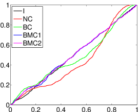
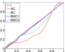
$\bm{p}=(3/5,1/5,1/5)$		$\bm{p}=(5/7,1/7,1/7)$

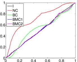
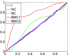
Figure 6: PITs cdf for different calibration models and different datasets.

More specifically, the two-component beta calibrations are able to achieve a more flexible deformation of the cdf linear combination providing a calibrated cdf (blue and magenta lines) which is close to the uniform cdf. Figure 7 shows the results of the calibration and combination procedure decomposed along the different components of the mixture. As an example consider the first dataset, generated with $\bm{p}=(1/5,1/5,3/5)$. The solid and dashed blue lines in the top-left plot of Figure 7 show the contribution of the first and second component respectively of the BMC1 mixture model to the calibration of the density. The first component mainly calibrates the pdf on the positive part of the support and the second component calibrates the pdf on the negative part of the support. Both components assign the same weights ($\omega=0.449$) to the first model in the pool, i.e. $\mathcal{N}(-1,1)$. This weight is higher than in the BC model, which has a less flexible calibration function and thus assigns a lower weight $\omega=0.202$ to the first model in the pool. The solid and dashed magenta lines in the top-left plot of Figure 7 show a behaviour similar to the BMC1 components.

$\bm{p}=(1/5,1/5,3/5)$		$\bm{p}=(1/7,1/7,5/7)$
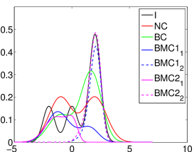
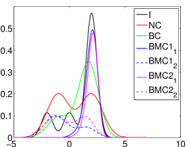
$\bm{p}=(3/5,1/5,1/5)$		$\bm{p}=(1/7,1/7,5/7)$

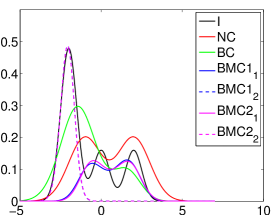
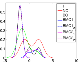
Figure 7: Contribution of the calibration components for different models BC, BMC1 (first and second mixture component, $BMC1_{1}$ and $BMC1_{2}$) and BMC2 (first and second mixture component, $BMC2_{1}$ and $BMC2_{2}$), and different datasets.

The first BMC2 component assigns weight $\omega_{1}=0.043$ to the first model in the pool. This means that the calibration on the negative part of the support set is done mainly using the predictive distribution of the second model, $\mathcal{N}(2,1)$. The calibration of the positive part of the set is obtained thanks to the second BMC2 component which assigns weight $\omega_{2}=0.667$ to the first model in the pool.

S4.2 Heavy Tails

Fig 8 focuses on the right tail of the predictive pdf and shows results for the calibrated and beta calibrated PITs cdf and their 99% HPD. There is strong evidence of the difficulties of the BC model in calibrating the tails. The BC underestimates the tail probability and over-estimates the central part of the distribution. The BMC1 and BMC2 models are able instead to provide well-calibrated PITs on the tails of the distribution.

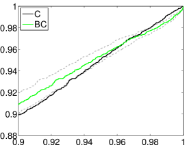
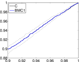
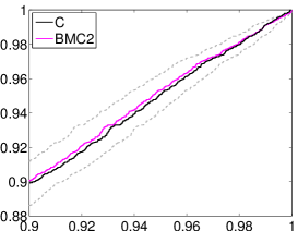
Figure 8: Results of the Bayesian calibration model BC (top), BMC1 (middle) and BMC2 (bottom) for the right tail of the predictive distribution. In each plot the PITs cdf of the calibrated (solid black line) and beta calibrated model (solid coloured line) and their 99% HPD region (gray dashed lines)

Appendix S5 Further real data results

References

- Abramowitz and Stegun, (1972) Abramowitz, M. and Stegun, I. A. (1972). Handbook of Mathematical Functions with Formulas, Graphs, and Mathematical Tables. Dover, New York.
- Altomare and Campiti, (1994) Altomare, F. and Campiti, M. (1994). Korovkin-type Approximation Theory and Its Application. De Gruyter, Berlin.
- Antoniak, (1974) Antoniak, C. E. (1974). Mixtures of Dirichlet processes with applications to Bayesian nonparametric problems. Annals of Statistics, 2:1152–1174.
- Artzner et al., (1999) Artzner, P., Delbaen, F., Eber, J., and Heath, D. (1999). Coherent measures of risk. Mathematical Finance, 9(3):203–228.
- Azzalini and Capitanio, (2003) Azzalini, A. and Capitanio, A. (2003). Distributions generated by perturbation of symmetry with emphasis on a multivariate skew t-distribution. Journal of the Royal Statistical Society, Series B, 65(2):367–389.
- Bassetti et al., (2014) Bassetti, F., Casarin, R., and Leisen, F. (2014). Beta-product dependent Pitman-Yor processes for Bayesian inference. Journal of Econometrics, 180:49–72.
- Bates and Granger, (1969) Bates, J. M. and Granger, C. W. J. (1969). Combination of forecasts. Operational Research Quarterly, 20:451–468.
- Billio and Casarin, (2011) Billio, M. and Casarin, R. (2011). Beta autoregressive transition Markov-switching models for business cycle analysis. Studies in Nonlinear Dynamics and Econometrics, 15:1–32.
- Billio et al., (2013) Billio, M., Casarin, R., Ravazzolo, F., and Van Dijk, H. (2013). Time-varying combinations of predictive densities using nonlinear filtering. Journal of Econometrics, 177:213–232.
- Bouguila et al., (2006) Bouguila, N., Ziou, D., and Monga, E. (2006). Practical Bayesian estimation of a finite beta mixture through Gibbs sampling and its applications. Statistics and Computing, 16:215–225.
- Burda et al., (2014) Burda, M., Harding, M., and Hausman, J. (2014). A Bayesian semiparametric competing risk model with unobserved heterogeneity. Journal of Applied Econometrics.
- Casarin et al., (2012) Casarin, R., Dalla Valle, L., and Leisen, F. (2012). Bayesian model selection for beta autoregressive processes. Bayesian Analysis, 7:1–26.
- Casarin et al., (2015) Casarin, R., Leisen, F., Molina, G., and ter Horst, E. (2015). A Bayesian beta markov random field calibration of the term structure of implied risk neutral densities. Bayesian Analysis, 10(4):791–819.
- Chib and Hamilton, (2002) Chib, S. and Hamilton, B. H. (2002). Semiparametric bayes analysis of longitudinal data treatment models. Journal of Econometrics, 110:67–89.
- Choudhuri et al., (2004) Choudhuri, N., Ghosal, S., and Roy, A. (2004). Bayesian estimation of the spectral density of a time series. Journal of the American Statistical Association, 99(468):1050–1059.
- Dawid, (1982) Dawid, A. P. (1982). The well-calibrated Bayesian. Journal of the American Statistical Association, 77(379):605–610.
- Dawid, (1984) Dawid, A. P. (1984). Statistical theory: The prequential approach. Journal of the Royal Statistical Society Series A, 147:278–290.
- Diaconis and Ylvisaker, (1985) Diaconis, P. and Ylvisaker, D. (1985). Quantifying prior opinion. In Bernardo, J. M., De Groot, M. H., Lindley, D. V., and Smith, A. F. M., editors, Bayesian Statistics 2. North Holland Amsterdam.
- Diebold et al., (1998) Diebold, F. X., Gunther, T. A., and Tay, A. S. (1998). Evaluating density forecasts with applications to financial risk management. International Economic Review, 39:863–883.
- Epstein, (1966) Epstein, E. S. (1966). Quality control for probability forecasts. Monthly Weather Review, 94:487–494.
- Escobar, (1994) Escobar, M. D. (1994). Estimating normal means with a Dirichlet process prior. Journal of the American Statistical Association, 89:268–277.
- Escobar and West, (1995) Escobar, M. D. and West, M. (1995). Bayesian density estimation and inference using mixtures. Journal of the American Statistical Association, 90:577–588.
- Ferguson, (1973) Ferguson, T. S. (1973). A Bayesian analysis of some nonparametric problems. Annals of Statistics, 1:209–230.
- French, (1996) French, S. (1996). Calibration and the expert problem. Management Science, 32(3):315–321.
- Frühwirth-Schnatter, (2006) Frühwirth-Schnatter, S. (2006). Finite Mixture and Markov Switching Models. Springer-Verlag, Berlin.
- Geweke, (2010) Geweke, J. (2010). Complete and Incomplete Econometric Models. Princeton University Press, Princeton.
- Geweke and Amisano, (2010) Geweke, J. and Amisano, G. (2010). Comparing and evaluating Bayesian predictive distributions of asset returns. International Journal of Forecasting, 26:216–230.
- Geweke and Amisano, (2011) Geweke, J. and Amisano, G. (2011). Optimal prediction pools. Journal of Econometrics, 164:130–141.
- Ghosal and van der Vaart, (2007) Ghosal, S. and van der Vaart, A. (2007). Posterior convergence rates of Dirichlet mixtures at smooth densities. Ann. Statist., 35(2):697–723.
- Ghosh and Ramamoorthi, (2003) Ghosh, J. K. and Ramamoorthi, R. V. (2003). Bayesian nonparametrics. Springer Series in Statistics. Springer-Verlag, New York.
- Gneiting et al., (2007) Gneiting, T., Balabdaoui, F., and Raftery, A. E. (2007). Probabilistic forecasts, calibration and sharpness. Journal of the Royal Statistical Society Series B, 69:243–268.
- Gneiting and Katzfuss, (2014) Gneiting, T. and Katzfuss, M. (2014). Probabilistic forecasting. Annual Review of Statistics and Its Application, 1:125–151.
- Gneiting and Ranjan, (2013) Gneiting, T. and Ranjan, R. (2013). Combining predictive distributions. Electronic Journal of Statistics, 7:1747–1782.
- Granger and Ramanathan, (1984) Granger, C. W. J. and Ramanathan, R. (1984). Improved methods of combining forecasts. Journal of Forecasting, 3:197–204.
- Griffin, (2011) Griffin, J. E. (2011). Inference in infinite superpositions of non-Gaussian Ornstein-Uhlenbeck processes using Bayesian nonparametric methods. Journal of Financial Econometrics, 1:1–31.
- Griffin and Steel, (2006) Griffin, J. E. and Steel, M. F. J. (2006). Order-based dependent Dirichlet processes. Journal of the American Statistical Association, 101:179–194.
- Griffin and Steel, (2011) Griffin, J. E. and Steel, M. F. J. (2011). Stick-breaking autoregressive processes. Journal of Econometrics, 162:383–396.
- Gzyl and Mayoral, (2008) Gzyl, H. and Mayoral, S. (2008). Determination of risk pricing measures from market prices of risk. Insurance: Mathematics and Economics., 43(3):437–443.
- Hall and Mitchell, (2007) Hall, S. G. and Mitchell, J. (2007). Combining density forecasts. International Journal of Forecasting, 23:1–13.
- Hatjispyros et al., (2011) Hatjispyros, S. J., Nicoleris, T. N., and Walker, S. G. (2011). Dependent mixtures of Dirichlet processes. Computational Statistics & Data Analysis, 55:2011–2025.
- Hirano, (2002) Hirano, K. (2002). Semiparametric Bayesian inference in autoregressive panel data models. Econometrica, 70:781–799.
- Hjort et al., (2010) Hjort, N. L., Homes, C., Müller, P., and Walker, S. G. (2010). Bayesian Nonparametrics. Cambridge University Press.
- Hoeting et al., (1999) Hoeting, J. A., Madigan, D., Raftery, A. E., and Volinsky, C. T. (1999). Bayesian model averaging: A tutorial. Statistical Science, 14:382–417.
- Ishwaran and James, (2001) Ishwaran, H. and James, L. F. (2001). Gibbs sampling methods for stick-breaking priors. Journal of the American Statistical Association, 96:161–173.
- Ishwaran and Zarepour, (2000) Ishwaran, H. and Zarepour, M. (2000). Markov chain Monte Carlo in approximate Dirichlet and beta two-parameter process hierarchical models. Biometrika, 87:371–390.
- Jensen and Maheu, (2010) Jensen, J. M. and Maheu, M. J. (2010). Bayesian semiparametric stochastic volatility modeling. Journal of Econometrics, 157:306–316.
- Jochmann, (2015) Jochmann, M. (2015). Modeling U.S. inflation dynamics: A Bayesian nonparametric approach. Econometric Reviews, 34(5):537–558.
- Jore et al., (2010) Jore, A. S., Mitchell, J., and Vahey, S. P. (2010). Combining forecast densities from VARs with uncertain instabilities. Journal of Applied Econometrics, 25:621–634.
- Kalli et al., (2011) Kalli, M., Griffin, J. E., and Walker, S. G. (2011). Slice sampling mixture models. Statistics and Computing, 21:93–105.
- Kapetanios et al., (2015) Kapetanios, G., Mitchell, J., Price, S., and Fawcett, N. (2015). Generalised density forecast combinations. Journal of Econometrics, 188:150–165.
- Kling and Bessler, (1989) Kling, J. L. and Bessler, D. A. (1989). Calibration-based predictive distributions: An application of prequential analysis to interest rates, money, prices, and output. Journal of Business, 62:477–499.
- Lerch and Thorarinsdottir, (2013) Lerch, S. and Thorarinsdottir, T. L. (2013). Comparison of nonhomogeneous regression models for probabilistic wind speed forecasting. Tellus Series A, 65:21206.
- Lo, (1984) Lo, A. Y. (1984). On a class of Bayesian nonparametric estimates: I. Density estimates. Annals of Statistics, 12:351–357.
- MacEachern and Müller, (1998) MacEachern, S. N. and Müller, P. (1998). Estimating mixtures of Dirichlet process models. Journal of Computational and Graphical Statistics, 7:223–238.
- Mitchell and Wallis, (2011) Mitchell, J. and Wallis, K. F. (2011). Evaluating density forecasts: Forecast combinations, model mixtures, calibration and sharpness. Journal of Applied Econometrics, 26:1023–1040.
- Molteni et al., (1996) Molteni, F., Buizza, R., Palmer, T. N., and Petroliagis, T. (1996). The ECMWF ensemble prediction system: Methodology and validation. Quarterly Journal of the Royal Meteorological Society, 122:73–119.
- Müller et al., (2004) Müller, P., Quintana, F., and Rosner, G. (2004). A method for combining inference across related nonparametric Bayesian models. Journal of the Royal Statistical Society B, 66:735–749.
- Norets and Pelenis, (2014) Norets, A. and Pelenis, J. (2014). Posterior consistency in conditional density estimation by covariate dependent mixtures. Econometric Theory, 30(3):606–646.
- Papaspiliopoulos and Roberts, (2008) Papaspiliopoulos, O. and Roberts, G. (2008). Retrospective Markov chain Monte Carlo for Dirichlet process hierarchical models. Biometrika, 95:169–186.
- Pelenis, (2014) Pelenis, J. (2014). Bayesian regression with heteroscedastic error density and parametric mean function. Journal of Econometrics, 178:624–638.
- Ranjan and Gneiting, (2010) Ranjan, R. and Gneiting, T. (2010). Combining probability forecasts. Journal of the Royal Statistical Society Series B, 72:71–91.
- Robert and Rousseau, (2002) Robert, C. P. and Rousseau, J. (2002). A mixture approach to Bayesian goodness of fit. Technical Report 02009, CEREMADE, Université Paris-Dauphine.
- Rodriguez and ter Horst, (2008) Rodriguez, A. and ter Horst, E. (2008). Bayesian dynamic density estimation. Bayesian Analysis, 3:339–366.
- Sethuraman, (1994) Sethuraman, J. (1994). A constructive definition of Dirichlet priors. Statistica Sinica, 4:639–650.
- Spiegelhalter et al., (2004) Spiegelhalter, D. J., Abrams, K. R., and Myles, J. P. (2004). Bayesian Approaches to Clinical Trials and Health-Care Evaluation. Wiley, Chichester.
- Stone, (1961) Stone, M. (1961). The linear pool. Annals of Mathematical Statistics, 2:1339–1342.
- Taddy, (2010) Taddy, M. A. (2010). Autoregressive mixture models for dynamic spatial Poisson processes: Application to tracking the intensity of violent crime. Journal of the American Statistical Association, 105:1403–1417.
- Taddy and Kottas, (2009) Taddy, M. A. and Kottas, A. (2009). Markov switching Dirichlet process mixture regression. Bayesian Analysis, 4:793–816.
- Tang and Ghosal, (2007) Tang, Y. and Ghosal, S. (2007). Posterior consistency of Dirichlet mixtures for estimating a transition density. J. Statist. Plann. Inference, 137(6):1711–1726.
- Tang et al., (2007) Tang, Y., Ghosal, S., and Roy, A. (2007). Nonparametric Bayesian estimation of positive false discovery rates. Biometrics, 63(4):1126–1134, 1312.
- Tay and Wallis, (2000) Tay, A. S. and Wallis, K. F. (2000). Density forecasting: A survey. Journal of Forecasting, 19:235–254.
- Walker, (2007) Walker, S. G. (2007). Sampling the Dirichlet mixture model with slices. Communications in Statistics – Simulation and Computation, 36:45–54.
- Wang and Young, (1998) Wang, S. and Young, V. (1998). Risk-adjusted credibility premiums using distorted probabilities. Scandinavian Actuarial Journal, 2:143–165.
- Wasserman, (2000) Wasserman, L. (2000). Asymptotic inference for mixture models using data-dependent priors. Journal of the Royal Statistical Society Series B, 62:159–180.
- West, (1992) West, M. (1992). Modelling agent forecast distributions. Journal of the Royal Stati, 54(2):553–567.
- West and Crosse, (1992) West, M. and Crosse, J. (1992). Modelling probabilistic agent opinion. Journal of the Royal St, 54(1):285–299.
- Wiesenfarth et al., (2014) Wiesenfarth, M., C.M., H., Kneib, T., and Cadarso-Suarez, C. (2014). Bayesian nonparametric instrumental variables regression based on penalized splines and dirichlet process mixtures. Journal of Business and Economic Statistics, 32(3):468–482.
- (78) Wu, Y. and Ghosal, S. (2009a). Correction to: “Kullback Leibler property of kernel mixture priors in Bayesian density estimation” [mr2399197]. Electron. J. Stat., 3:316–317.
- (79) Wu, Y. and Ghosal, S. (2009b). Kullback Leibler property of kernel mixture priors in Bayesian density estimation. Electron. J. Stat., 2:298–331.