UMISS-HEP-2015-01
Decay in the Standard Model and with New Physics
Shanmuka Shivashankara 111sshivash@go.olemiss.edu,
Wanwei Wu 222wwu1@go.olemiss.edu and
Alakabha Datta 333datta@phy.olemiss.edu
Department of Physics and
Astronomy, 108 Lewis Hall,
University of Mississippi, Oxford, MS
38677-1848, USA
()
Abstract
Recently hints of
lepton flavor non-universality emerged when the BaBar Collaboration
observed deviations from the standard model predictions in (). Another test of this non-universality can be in the semileptonic
decay. In this work we present predictions for this decay in the standard model
and in the presence of
new-physics operators with different Lorentz structures. We present the most general four-fold angular distribution for this decay including new physics. For phenomenology, we focus on
predictions for the decay rate and the differential distribution in the momentum transfer
squared . In particular, we calculate where
represents or , and find the standard model prediction to be around
while the new physics operators can increase or slightly decrease this value.
1 Introduction
A major part of particle physics research is focused on finding physics beyond the standard model (SM). In the flavor sector a key property of the SM gauge interactions is that they are lepton flavor universal. Evidence for violation of this property would be a clear sign of new physics (NP) beyond the SM. In the search for NP, the second and third generation quarks and leptons are quite special because they are comparatively heavier and are expected to be relatively more sensitive to NP. As an example, in certain versions of the two Higgs doublet models (2HDM) the couplings of the new Higgs bosons are proportional to the masses and so NP effects are more pronounced for the heavier generations. Moreover, the constraints on new physics, especially involving the third generation leptons and quarks, are somewhat weaker allowing for larger new physics effects.
Recently, the BaBar Collaboration with their full data sample has reported the following measurements [1, 2]:
| (1) |
where . The SM predictions are and [1, 3], which deviate from the BaBar measurements by 2 and 2.7, respectively. (The BaBar Collaboration itself reported a 3.4 deviation from SM when the two measurements of Eq. (1) are taken together.) This measurement of lepton flavor non-universality, referred to as the puzzles, may be providing a hint of the new physics (NP) believed to exist beyond the SM. There have been numerous analyses examining NP explanations of the measurements [3, 4, 5, 6].
The underlying quark level transition can be probed in both and decays. Note that in the presence of lepton non-universality the flavor of the neutrino does not have to match the flavor of the charged lepton [6]. Moreover the NP can affect all the lepton flavors. The main assumption here is that the NP effect is largest for the sector and for simplicity we neglect the smaller NP effects in the and leptons. The being a spin 1/2 baryon has a complex angular distribution for its decay products. As in decays, we can construct several observables from the angular distribution of the decay which can be used to find evidence of NP and to probe the structure of NP.
The decay has not been measured experimentally though it might be possible to observe this decay at the LHCb. The full angular distribution of this decay is experimentally challenging and so in this paper, for the sake of phenomenology, we will focus on the rate as well as the differential distribution for this decay. Using constraints on the new physics couplings obtained by using Eq. (1) we will make predictions for the effects of these couplings in decay. Recently, in Ref. [7] this decay was discussed in the standard model and with new physics in Ref. [8].
The main uncertainty in the decays are the hadronic form factors for the transition. These form factors can also be studied systematically in a heavy and expansion [9]. However, unlike the system the heavy baryon form factors have not been extensively studied. We will therefore construct ratios where the form factor uncertainties will mostly cancel leaving behind a smaller uncertainty for the theoretical predictions. We will then investigate if the NP effects are large enough to produce observable deviations from the SM predictions.
The paper is organized in the following manner. In sec.2 we introduce the effective Lagrangian to parametrize the NP operators, describe the formalism of the decay process and introduce the relevant observables. In sec.3 we present our results and in sec.4 we present our conclusions.
2 Formalism
In the presence of NP, the effective Hamiltonian for the quark-level transition can be written in the form [10]
| (2) | |||||
where is the Fermi coupling constant, is the Cabibbo-Koboyashi-Maskawa (CKM) matrix element and we use . We have assumed the neutrinos to be always left chiral and to introduce non-universality the NP couplings are in general different for different lepton flavors. We assume the NP effect is mainly through the lepton and do not consider tensor operators in our analysis. Further, we do not assume any relation between and transitions and hence do not include constraints from . The SM effective Hamiltonian corresponds to .
In Ref.[5] we had parametrized the NP in terms of the couplings , , and while in this work we have traded and for to align our analysis closer to realistic models [6]. The couplings contribute to while contribute to . We will consider one NP coupling at a time and provide constraints on these couplings from .
2.1 Decay Process
The process under consideration is
In the SM the amplitude for this process is
| (3) |
where the leptonic and hadronic currents are,
| (4) |
The hadronic current is expressed in terms of six form factors,
| (5) |
Here is the momentum transfer and the form factors are functions of . When considering NP operators we will use the following relations obtained by using the equations of motion.
| (6) |
We will define the following observable,
| (7) |
Here represents or . We will also define the ratio of differential distributions,
| (8) |
Our results will show that these observables are not very sensitive to variations in the hadronic form factors.
2.2 Helicity Amplitudes and the Full Angular Distribution
The decay proceeds via (off-shell W) followed by . The full decay process is Following [11] one can analyze the decay in terms of helicity amplitudes which are given by
| (9) |
where are the polarizations of the daughter baryon and the W-boson respectively and is the hadronic current for transition. The helicity amplitudes can be expressed in terms of form factors and the NP couplings.
| (10) |
where .
We also have,
| (11) |
The scalar and pseudo-scalar helicities associated with the new physics scalar and pseudo-scalar interactions are
| (12) |
The parity related amplitudes are,
| (13) |
With the W boson momentum defining the positive z-axis for the decay process (), the twofold angular distribution can be written as
| (14) | |||||
where,
| (15) | |||||
, , , and are the standard model non-spin-flip, standard model spin-flip, new physics, and interference terms, respectively apart from and . Note , have the same structure as the SM contributions but the helicity amplitudes in these quantities include the new physics contributions from . is the angle of the lepton in the W rest frame with respect to the W momentum.
After integrating out ,
| (16) | |||||
where,
| (17) |
, , , and are the standard model non-spin-flip, standard model spin-flip, new physics, and interference terms, respectively apart from and . Again, , have the same structure as the SM contributions but the helicity amplitudes in these quantities include the new physics contributions from . The operators generate new terms in the angular distribution.
The angular distribution for the four body decay process () can be written as the following where is the parity parameter for the process . is again the same leptonic angle. is the angle of in the rest frame with respect to the momentum. is the dihedral angle between the decay planes of () and () in the W and rest frame, respectively.
| (18) | |||||
where,
| (19) | |||||
, , , and are the standard model non-spin-flip, standard model spin-flip, new physics, and interference terms, respectively apart from and . and have the same structure as the SM contributions but the helicity amplitudes in these quantities include the new physics contributions from . Several additional observables can be constructed from the angular distributions, such as polarization asymmetries and CP violating triple product asymmetries [12] which can be sensitive probes of new physics. Note that the standard model portion of the twofold and fourfold distributions above, Eq. 14 and Eq. 18, are the same as in a recent paper[7] apart from a minus sign in above. 444In [7] Eq. (51), the minus sign is required in front of sin2 on the second line in the spin-flip term as can be seen by the elements.
3 Numerical Results
3.1 New Physics Couplings
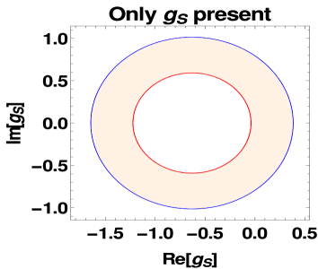
We first present the constraints on the NP couplings from . The couplings only contributes to , only contributes to while contributes to both and . The details of the calculations for Fig. 1 can be found in Ref. [3, 5].


3.2 Form Factors
One of the main inputs in our calculations are the form factors. As first principle, lattice calculations of the form factors are not yet available. The form factors we use here are from QCD sum rules, which is a well known approach to compute non-perturbative effects like form factors for systems with both light and heavy quarks[13, 14].
In Ref. [14], various parametrizations of the form factors are used. They are shown in Table. 1 ( ).
| continuum model | |||
|---|---|---|---|
| rectangular | 1 | ||
| rectangular | 2 | ||
| triangular | 3 | ||
| triangular | 4 |
The form factors satisfy the heavy quark effective theory relations in the limit.
| (20) |
3.3 Graphs and Results
We have used the following masses in our calculations. The masses of the particles are GeV, GeV, GeV, GeV, GeV, GeV and [15].
In the following we present the results for , and . For the first and third observables we use different models of the form factors given in Table.1. For the differential distribution we present the average result over the form factors.
| continuum model | 1 | 2 | 3 | 4 | Average | Ref. [7] | Ref. [8] | Ref. [16] |
|---|---|---|---|---|---|---|---|---|
| 0.31 | 0.29 | 0.28 | 0.28 | 0.29 | 0.31 |
We first present our prediction for in the SM, in Table. 2, for the various choices of the form factors in Table.1. We also compare our results with other calculations of this quantity by other groups using different form factors. We find the average value for in the SM, . This agrees very well with values for this quantity obtained in Ref. [7] which uses a covariant confined quark model for the form factors, Ref. [8] which uses the form factor model in Ref. [17], and Ref. [16] which uses the lattice QCD. This confirms our earlier assertion that the ratio is largely free from form factor uncertainties making it an excellent probe to find new physics.
We now discuss our results. From the structure of Eq. 16 we can make some general observations. We start with the case where only is present. In this case the NP has the same structure as the SM and the SM amplitude gets modified by the factor [6]. Hence, if only is present then
| (21) |
Therefore in this case and we find the range of to be . The shape of the differential distribution is the same as the SM. In the left-side figures of Fig. 2 we show the plots for , and when only is present. We then consider the case where only is present. If only is present then from Eq. 2.2,
| (22) |
In this case no clear relation between and can be obtained. However, for the allowed couplings we find is greater than the SM value and is in the range . The shape of the differential distribution is the same as the SM. In the right-side figures of Fig. 2 we show the plots for , and when only is present.
We now move to the case when only are present. Using Eq. 16 and Eq. 2.2 we can write,
| (23) |
The quantities and depend on masses and form factors and they are positive. Hence for or , is always greater than or equal to . But, for or , can be less than the SM value. However, given the constraints on we can make only slightly less than the SM value. We find is in the range when only is present and in the range when only is present.
In Fig. 3 we show the plots for , and when only is present. The shape of the differential distribution can be different from the SM. In Fig. 4 we show the plots for , and when only is present. In this case also the shape of the differential distribution can be different from the SM.
| NP | ||
|---|---|---|
| Only | , | , |
| Only | , | , |
| Only | , | , |
| Only | , | , |
In Table. 3 we show the minimum and maximum values for the averaged with the corresponding NP couplings.


4 Conclusion
In this paper we calculated the SM and NP predictions for the decay . Motivation to study this decay comes from the recent hints of lepton flavor non-universality observed by the BaBar Collaboration in (). We used a general parametrization of the NP operators and fixed the new physics couplings from the experimental measurements of and . We then made predictions for ( Eq.7), , and ( Eq.8) for the various NP couplings taken one at a time. We found the interesting result that couplings gave predictions larger than the SM values for all the three observables. We found the couplings to produce larger effects than the couplings. We also provided the general formula for the various angular distributions in the presence of NP operators.
Acknowledgments: This work was financially supported in part by the National Science Foundation under Grant No.NSF PHY-1414345. We thank Jrgen Krner, Preet Sharma, and Sheldon Stone for useful discussions.
References
- [1] J. P. Lees et al. [BaBar Collaboration], Phys. Rev. Lett. 109, 101802 (2012) [arXiv:1205.5442 [hep-ex]].
- [2] J. P. Lees et al. [BaBar Collaboration], Phys. Rev. D 88, 072012 (2013) [arXiv:1303.0571 [hep-ex]].
- [3] S. Fajfer, J. F. Kamenik and I. Nisandzic, [arXiv:1203.2654 [hep-ph]]; Y. Sakaki and H. Tanaka, [arXiv:1205.4908 [hep-ph]].
- [4] S. Fajfer, J. F. Kamenik, I. Nisandzic and J. Zupan, Phys. Rev. Lett. 109, 161801 (2012) [arXiv:1206.1872 [hep-ph]]; A. Crivellin, C. Greub and A. Kokulu, Phys. Rev. D 86, 054014 (2012) [arXiv:1206.2634 [hep-ph]]; D. Becirevic, N. Kosnik and A. Tayduganov, Phys. Lett. B 716, 208 (2012) [arXiv:1206.4977 [hep-ph]]; N. G. Deshpande and A. Menon, [arXiv:1208.4134 [hep-ph]]; A. Celis, M. Jung, X. -Q. Li and A. Pich, JHEP 1301, 054 (2013) [arXiv:1210.8443 [hep-ph]]; D. Choudhury, D. K. Ghosh and A. Kundu, Phys. Rev. D 86, 114037 (2012) [arXiv:1210.5076 [hep-ph]]; M. Tanaka and R. Watanabe, [arXiv:1212.1878 [hep-ph]]; P. Ko, Y. Omura and C. Yu, [arXiv:1212.4607 [hep-ph]]; Y. -Y. Fan, W. -F. Wang and Z. -J. Xiao, [arXiv:1301.6246 [hep-ph]]; P. Biancofiore, P. Colangelo and F. De Fazio, [arXiv:1302.1042 [hep-ph]]; A. Celis, M. Jung, X. -Q. Li and A. Pich, [arXiv:1302.5992 [hep-ph]]; I. Dorsner, S. Fajfer, N. Kosnik and I. Nisandzic, JHEP 1311, 084 (2013) [arXiv:1306.6493 [hep-ph]]; Y. Sakaki, M. Tanaka, A. Tayduganov and R. Watanabe, Phys. Rev. D 88, 094012 (2013) [arXiv:1309.0301 [hep-ph]], [arXiv:1412.3761 [hep-ph]]; Y. Sakaki, M. Tanaka, A. Tayduganov and R. Watanabe, [arXiv:1412.3761 [hep-ph]].
- [5] A. Datta, M. Duraisamy and D. Ghosh, Phys. Rev. D 86, 034027 (2012) [arXiv:1206.3760 [hep-ph]]; M. Duraisamy and A. Datta, JHEP 1309, 059 (2013) [arXiv:1302.7031 [hep-ph]]; M. Duraisamy, P. Sharma and A. Datta, Phys. Rev. D 90, 074013 (2014) [arXiv:1405.3719 [hep-ph]].
- [6] B. Bhattacharya, A. Datta, D. London and S. Shivashankara, Phys. Lett. B 742, 370 (2015) [arXiv:1412.7164 [hep-ph]].
- [7] T. Gutsche, M. A. Ivanov, J. G. Korner, V. E. Lyubovitskij, P. Santorelli and N. Habyl, arXiv:1502.04864 [hep-ph].
- [8] R. M. Woloshyn, PoS Hadron 2013, 203 (2013).
- [9] See for e.g. M. Neubert, ”Heavy-quark symmetry.”, Phy. Rep. 245, 259 (1994) [ arXiv:hep-ph/9306320]; A. Datta, Phys. Lett. B 349, 348 (1995) [hep-ph/9411306].
- [10] T. Bhattacharya, V. Cirigliano, S. D. Cohen, A. Filipuzzi, M. Gonzalez-Alonso, M. L. Graesser, R. Gupta and H. -W. Lin, Phys. Rev. D 85, 054512 (2012) [arXiv:1110.6448 [hep-ph]]; C. -H. Chen and C. -Q. Geng, Phys. Rev. D 71, 077501 (2005) [hep-ph/0503123].
- [11] J. G. Korner and M. Kramer, Phys. Lett. B 275, 495 (1992).
- [12] A. Datta and D. London, Int. J. Mod. Phys. A 19, 2505 (2004) [hep-ph/0303159]; W. Bensalem, A. Datta and D. London, Phys. Rev. D 66, 094004 (2002) [hep-ph/0208054]; W. Bensalem, A. Datta and D. London, Phys. Lett. B 538, 309 (2002) [hep-ph/0205009].
- [13] M.A.Shifman, A.I. Vainshtein and V.I. Zakharov, Nucl. Phys. B147, 385(1979); 448
- [14] De Carvalho, RS Marques, et al. ”Form factors and decay rates for heavy semileptonic decays from QCD sum rules.” Phys. Rev. D 60, 034009 (1999) [arXiv:hep-ph/9903326v1]
- [15] K.A. Olive et al. (Particle Data Group), Chin. Phys. C, 38, 090001 (2014).
- [16] W. Detmold, C. Lehner and S. Meinel, [arXiv:1503.01421 [hep-lat]].
- [17] M. Pervin, W. Roberts and S. Capstick, Phys. Rev. C 72, 035201 (2005) [nucl-th/0503030].