An analytical study of seismoelectric signals produced by 1D mesoscopic heterogeneities

This paper has been accepted for publication in Geophysical Journal International:

L. B. Monachesi, J. G. Rubino, M. Rosas-Carbajal, D. Jougnot, N. Linde, B. Quintal, K. Holliger (2015) An analytical study of seismoelectric signals produced by 1D mesoscopic heterogeneities, Geophys. J. Int., 201, 329 - 342, doi: 10.1093/gji/ggu482.

The presence of mesoscopic heterogeneities in fluid-saturated porous rocks can produce measurable seismoelectric signals due to wave-induced fluid flow between regions of differing compressibility. The dependence of these signals on the petrophysical and structural characteristics of the probed rock mass remains largely unexplored. In this work, we derive an analytical solution to describe the seismoelectric response of a rock sample, containing a horizontal layer at its center, that is subjected to an oscillatory compressibility test. We then adapt this general solution to compute the seismoelectric signature of a particular case related to a sample that is permeated by a horizontal fracture located at its center. Analyses of the general and particular solutions are performed to study the impact of different petrophysical and structural parameters on the seismoelectric response. We find that the amplitude of the seismoelectric signal is directly proportional to the applied stress, to the Skempton coefficient contrast between the host rock and the layer, and to a weighted average of the effective excess charge of the two materials. Our results also demonstrate that the frequency at which the maximum electrical potential amplitude prevails does not depend on the applied stress or the Skempton coefficient contrast. In presence of strong permeability variations, this frequency is rather controlled by the permeability and thickness of the less permeable material. The results of this study thus indicate that seismoelectric measurements can potentially be used to estimate key mechanical and hydraulic rock properties of mesoscopic heterogeneities, such as compressibility, permeability, and fracture compliance.

1 Introduction

Free electrical charges at the mineral surfaces of fluid-saturated porous rocks are responsible for an electrical double layer (EDL) in the pore space surrounding the solid grains. The EDL is characterized by an electrical excess charge that counter-balances the surface charges (Hunter, 1981). Pore fluid flow in response to a propagating seismic wave (Biot, 1956a, b) exerts a drag on this excess charge, thus resulting in an electrical source current generally referred to as streaming current. This in turn results in an electrical potential distribution, which can be measured in laboratory and field experiments. The thus generated electric field depends on a range of important petrophysical parameters, such as the porosity, the permeability, and the type of saturating fluid. This has fostered an increased interest in this physical process, commonly referred to as seismoelectric conversion (e.g., Thompson & Gist, 1993; Jouniaux, 2011).

Pride (1994) developed the theoretical basis of the seismoelectric phenomenon by coupling Biot’s (1956a; 1956b) and Maxwell’s equations through a volume-averaging approach. This theory predicts two kinds of seismoelectric conversions: (1) the coseismic field and (2) the interface response. The coseismic field is a consequence of the wavelength-scale relative fluid flow associated with the passing seismic wavefield, which in turn generates a streaming current and thus an electric field. This field travels with the seismic wave, even in the case of homogeneous media, but is largely limited to the wave’s support volume (Pride & Haartsen, 1996). Conversely, the interface response occurs when a seismic perturbation strikes on an interface in terms of mechanical or electrical properties. In this case, a variation in the streaming current distribution arises, breaking the symmetry in the charge separation. This generates an electromagnetic (EM) signal that propagates independently of the seismic wave and can be measured outside the support volume of the wave, thus allowing for the remote detection of geological interfaces. These signals are highly sensitive to the fluid pressure gradients in the vicinity of the interface. Thus, proper modeling of wave conversions at interfaces, and in particular of Biot slow waves, is critical for the accurate modeling of seismolectric interface responses (Pride & Garambois, 2002).

The propagation of seismic waves through a medium containing mesoscopic heterogeneities, that is, heterogeneities having sizes larger than the typical pore scale but smaller than the prevailing wavelengths, can produce significant oscillatory fluid flow, generally referred to as wave-induced fluid flow, between the different regions composing the heterogeneous medium (e.g., Müller et al., 2010). Due to the differing elastic compliances of the various regions, the stresses associated with the seismic perturbation produce a pore fluid pressure gradient and, consequently, fluid flow. The energy dissipation related to this phenomenon is considered to be one of the most common and important seismic attenuation mechanisms in the shallower parts of the crust (e.g., Müller et al., 2010). Given that the amount of fluid flow produced by this phenomenon can be significant, a potentially important interface-type seismoelectric signal is also expected to arise. However, the nature and importance of the seismoelectric effects related to mesoscopic heterogeneities remain largely unexplored. An interesting study of this kind was presented by Haartsen & Pride (1997) who modeled the seismoelectric response of a single sand layer having a thickness much smaller than the predominant seismic wavelength and embedded in a less permeable medium. They observed that while the seismic amplitudes recorded at the surface were very small due to destructive interferences, the converted EM amplitudes were significantly enhanced compared to the case of a thick sand layer. More recently, Jougnot et al. (2013) proposed a numerical framework to study the seismoelectric response of a rock sample containing mesoscopic fractures subjected to an oscillatory compressibility test (Rubino et al., 2009, 2013) and found seismoelectric signals that would be measurable for typical laboratory setups (e.g., Tisato & Quintal, 2013). These findings are important not only as the seismoelectric responses of most geological environments are expected to contain a component related to fluid flow at mesoscopic scale, but also because they open the perspective of developing seismoelectric spectroscopy as a novel laboratory method for characterizing heterogeneous porous media. Jougnot et al. (2013) suggest that a better understanding of the role played by mesoscopic heterogeneities could help to improve some of the practical aspects of the seismoelectric method, such as the notoriously high noise levels generally observed in the measurements.

In this work, we present an analytical approach to study the origin of the seismoelectric signal produced by mesoscopic heterogeneities. We first derive a general analytical solution for the seismoelectric response of a homogeneous rectangular rock sample containing a horizontal layer at its center and subjected to an oscillatory compressibility test. Following Brajanovski et al. (2005), we then adapt the analytical solution to the particular case of a sample containing a central layer having thickness and dry-frame elastic moduli tending to zero in conjunction with porosity tending to one. This particular solution represents the response of a sample permeated by a horizontal fracture at its center. Finally, we employ these two solutions to explore the roles played by different petrophysical and structural properties in the seismoelectric signatures of heterogeneous rocks. This analysis may, in turn, help to identify which parameters could be retrieved from seismoelectric measurements.

2 Methodology

2.1 Oscillatory compressibility test

We consider a rectangular fluid-saturated porous rock sample containing a horizontal layer located at its center (Fig. 1). The two regions embedding this mesoscopic heterogeneity are identical. For simplicity, we choose the center of the sample as the origin of the $z$-axis and, therefore, the positions of the upper and lower boundaries of the heterogeneity are $z=L_{1}$ and $z=-L_{1}$, respectively. The thicknesses of the two embedding regions constituting the host rock are $L_{2}$ and the total thickness of the sample is $L=2(L_{1}+L_{2})$.

The sample is subjected to a time-harmonic compression of the form $\Delta Pe^{i\omega t}$ at its top boundary, with $\omega$ being the angular frequency, $t$ the time, and $i=\sqrt{-1}$ (Rubino et al., 2009, 2013). We impose that the solid phase is not allowed to move on the bottom boundary, nor to have horizontal displacements at the lateral boundaries and the pore fluid cannot flow into or out of the sample. For the considered geometry and boundary conditions, the problem to solve is 1D. We consider frequencies $\omega$ smaller than Biot’s critical frequency $\omega_{B}$ (e.g., Biot, 1962)

$$\omega_{B}=2\pi f_{B}=\frac{\phi\eta}{\kappa\rho_{f}},$$ (1)

where $\phi$ is the porosity, $\kappa$ the permeability, $\rho_{f}$ the density of the pore fluid, and $\eta$ the fluid viscosity. In this frequency range, viscous boundary layer effects are negligible and thus we can solve Biot’s (1941) consolidation equations to obtain the response of the sample. In the 1D space-frequency domain these equations can be written as

$$\frac{\partial\tau}{\partial z}=0,$$ (2)

$$i\omega\frac{\eta}{\kappa}w=-\frac{\partial p_{f}}{\partial z},$$ (3)

where $\tau$ and $p_{f}$ denote the total stress and the fluid pressure, respectively, whereas $w$ is the relative fluid-solid displacement. Equation (2) represents the stress equilibrium within the sample, whereas Eq. (3) is Darcy’s law. These two equations are coupled through the 1D stress-strain relations

$$\tau=H\frac{\partial u}{\partial z}+\alpha M\frac{\partial w}{\partial z},$$ (4)

$$p_{f}=-\alpha M\frac{\partial u}{\partial z}-M\frac{\partial w}{\partial z}.$$ (5)

In these equations, $u$ denotes the average displacement of the solid phase and the coefficients $H$, $M$ and $\alpha$ are given by

$$H=\lambda+2\mu,$$ (6)

$$M=\left[\frac{\alpha-\phi}{K_{s}}+\frac{\phi}{K_{f}}\right]^{-1},$$ (7)

$$\alpha=1-\frac{K_{m}}{K_{s}},$$ (8)

where $K_{m}$, $K_{s}$, and $K_{f}$ are the bulk moduli of the solid matrix, solid grains, and fluid phase, respectively. Moreover, $\mu$ is the shear modulus of the bulk material, which is equal to that of the dry matrix, and $\lambda$ is the Lamé constant, given by

$$\lambda=K_{m}+M\alpha^{2}-\frac{2}{3}\mu.$$ (9)

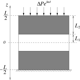
Figure 1: Schematic representation of a rectangular porous rock sample containing a horizontal layer (white rectangle) embedded between two identical regions (gray upper and lower rectangles). The sample is subjected to an oscillatory compressibility test.

For a homogeneous medium, combining Eqs. (2) and (4), as well as Eqs. (3) and (5) leads to

$$\frac{\partial^{2}u}{\partial z^{2}}=-\frac{\alpha M}{H}\frac{\partial^{2}w}{\partial z^{2}},$$ (10)

and

$$i\omega\frac{\eta}{\kappa}w=\alpha M\frac{\partial^{2}u}{\partial z^{2}}+M\frac{\partial^{2}w}{\partial z^{2}},$$ (11)

respectively. Next, substituting Eq. (10) into Eq. (11), results in

$$i\omega w=D\frac{\partial^{2}w}{\partial z^{2}}.$$ (12)

Equation (12) is a diffusion equation, with the diffusivity $D$ given by

$$D=\frac{\kappa N}{\eta},$$ (13)

where $N=M-\alpha^{2}M^{2}/H$.

The spatial scale at which wave-induced fluid flow is significant is determined by the diffusion length

$$L_{d}\equiv\sqrt{D/\omega}.$$ (14)

From Eqs. (13) and (14) it is clear that this length increases with increasing permeability and decreasing viscosity. When the diffusion length is of similar size as the characteristic size of the heterogeneities, $a_{meso}$, a characteristic frequency can be defined as

$$f_{c}\approx\frac{D}{2\pi\ a_{meso}^{2}},$$ (15)

which represents the limit between two types of mechanical behaviors in response to the oscillatory compression. For frequencies $f\ll f_{c}$, the diffusion lengths are much larger than the typical size of the heterogeneities. Correspondingly, there will be enough time during each oscillatory half-cycle for the pore fluid pressure to equilibrate at a common value. Thus, this low-frequency regime represents a relaxed state. For frequencies $f\gg f_{c}$, the diffusion lengths are very small compared to the size of the heterogeneities and, hence, there is no time for interaction between the pore fluids of the different parts of the rock. In this case, the pore pressure is approximately constant within each heterogeneity and, consequently, the high-frequency regime is associated with an unrelaxed state. For intermediate frequencies, $f\approx f_{c}$, significant fluid flow can be induced by an oscillatory stress field (e.g., Müller et al., 2010). From Eqs.  (13) and (15) we notice that the frequency range where significant fluid flow can occur shifts towards lower frequencies for decreasing permeability, increasing fluid viscosity, or increasing size of the heterogeneities.

The general solution of Eq. (12) for a homogeneous medium is given by

$$w(z)=Ae^{-kz}+Be^{kz},$$ (16)

where

$$k=\frac{\sqrt{i}}{L_{d}},$$ (17)

and $A$ and $B$ being complex-valued constants. From Eq. (4), given that $\tau$ is spatially constant in virtue of Eq. (2), the solid displacement can be expressed as

$$u(z)=-\beta w(z)+\frac{\tau}{H}z+C,$$ (18)

where $\beta\equiv\alpha M/H$ is the 1D Skempton coefficient (Appendix A) and $C$ is an additional complex-valued constant. Eqs. (16) to (18) then constitute the general solutions of Eqs. (2) to (5) for homogeneous media.

Since the generation of the seismoelectric signal is produced by the relative fluid velocity field, $i\omega w$, we seek an analytical expression for this parameter. The solid displacement $u$ always appears as a derivate with respect to $z$ in Eqs. (2) to (5). This means that if $\left(w(z),u(z)\right)$ constitute a solution for such equations, then $\left(w(z),u(z)+\chi\right)$, with $\chi$ being a constant, is also a solution. Hence, the solution for $w$ is independent of the solid displacement value imposed at the bottom boundary of the sample. Correspondingly, without changing the solution for $w$, we can modify the boundary condition imposed on $u$ at the bottom boundary to produce $u=0$ at $z=0$. Under this condition, and since $\tau$ is constant within the sample (Eq. (2)), it is clear that the geometry and the imposed boundary conditions are symmetrical with respect to $z=0$ and, therefore, the resulting fluid flow profile should also be symmetrical with respect to the center of the sample. Hence, we can simply solve Eq. (12) in the upper half of the sample shown in Fig. 1 under the following boundary conditions

$$\tau = -\Delta P,\quad\ \ \ z=L/2,$$ (19)

$$w = 0,\quad\ \ \ \ \ \ \ \ \ z=L/2,$$ (20)

$$w = 0,\quad\ \ \ \ \ \ \ \ \ z=0,$$ (21)

$$u = 0,\quad\ \ \ \ \ \ \ \ \ z=0.$$ (22)

According to Eqs. (16) and (18), the general solutions in the upper half of the sample can be expressed as

$$w_{j}(z) = A_{j}e^{-k_{j}z}+B_{j}e^{k_{j}z},$$ (23)

$$u_{j}(z) = -\beta_{j}w_{j}(z)-\frac{\Delta P}{H_{j}}z+C_{j},\qquad\qquad j=1,2,$$ (24)

where $\tau$ has been replaced by the imposed stress $-\Delta P$. The subscripts $1$ and $2$ denote the parameters of the lower ($0\leq z\leq L_{1}$) and upper ($L_{1}\leq z\leq L/2$) layers composing the upper half of the sample, respectively. The six unknowns $A_{j}$, $B_{j}$, and $C_{j}$ ($j=1,2$) are determined by imposing the conditions given by Eqs. (20) to (22) and the continuity of $u$, $w$, and $p_{f}$ at the interface $z=L_{1}$. Taking these six conditions into account and the fact that the relative fluid displacement $w$ is an odd function, it can be shown that

$$w(z)=\begin{cases}\begin{array}[]{lcl}sgn(z)A_{1}\left(e^{-k_{1}\lvert z\rvert}-e^{k_{1}\lvert z\rvert}\right),\quad\quad\quad\quad\quad\quad 0\leq\lvert z\rvert\leq L_{1},\\ sgn(z)A_{2}\left(e^{-k_{2}\lvert z\rvert}-e^{-k_{2}(L-\lvert z\rvert)}\right),\quad\quad\quad L_{1}\leq\lvert z\rvert\leq L/2,\end{array}\end{cases}$$ (25)

where $sgn$ is the sign function. The parameters $A_{1}$ and $A_{2}$ are given by

$$A_{1}=\left(e^{-k_{1}L_{1}}-e^{k_{1}L_{1}}\right)^{-1}\frac{\Delta P\left(\beta_{1}-\beta_{2}\right)}{\sum_{j=1}^{2}N_{j}k_{j}\ coth(k_{j}L_{j})},$$ (26)

$$A_{2}=\left(e^{-k_{2}L_{1}}-e^{-k_{2}(L-L_{1})}\right)^{-1}\frac{\Delta P\left(\beta_{1}-\beta_{2}\right)}{\sum_{j=1}^{2}N_{j}k_{j}\ coth(k_{j}L_{j})}.$$ (27)

In the following subsection, the above expressions for the relative fluid displacement are used to infer the distribution of the electrical potential within the sample in response to the applied oscillatory compression.

2.2 General solution: seismoelectric response of a rock sample containing a horizontal layer

When a relative displacement between the pore fluid and the solid frame occurs in response to the applied oscillatory compression, a drag on the electrical excess charges of the EDL takes place. This, in turn, generates a source or streaming current density $j_{s}$. Since the distributions of both the excess charge and the microscopic relative velocity of the pore fluid are highly dependent on their distance to the mineral grains, not all the excess charge is dragged at the same velocity by the flow. Correspondingly, an effective excess charge density $\bar{Q}_{v}^{\text{eff}}$ smaller than the total excess charge density $\bar{Q}_{v}$ has to be employed (e.g., Jougnot et al., 2012; Revil & Mahardika, 2013). In the considered 1D case, the source current density takes the form (e.g., Jardani et al., 2010; Jougnot et al., 2013)

$$j_{s}=\bar{Q}_{v}^{\text{eff}}i\omega w,$$ (28)

where $i\omega w$ is the relative fluid velocity. The effective excess charge formulation, which allows us to explicitly express the role played by the relative fluid velocity in the source current density generation, is equivalent to the electrokinetic coupling coefficient formulation commonly used in the seismoelectric literature (e.g., Pride, 1994). The relationship between the effective excess charge and the electrokinetic coupling coefficient can be found in many works such as Revil & Leroy (2004), Jougnot et al. (2012), or Revil & Mahardika (2013).

In the absence of an external current density, the 1D electrical potential $\varphi$ in response to a given source current density satisfies (Sill, 1983)

$$\frac{\partial}{\partial z}\left(\sigma\frac{\partial\varphi}{\partial z}\right)=\frac{\partial j_{s}}{\partial z},$$ (29)

where $\sigma$ denotes the electrical conductivity, which strongly depends on the saturating fluid as well as on textural properties of the medium, such as porosity and tortuosity.

The approach presented above is based on the fact that the electrical potential field has a negligible effect on the fluid flow pattern and, therefore, the seismic and electrical problems can be assumed to be decoupled. This assumption is made in most seismoelectric studies for materials similar to the ones considered in this work (e.g., Haines & Pride, 2006; Guan & Hu, 2008; Zyserman et al., 2010).

In order to obtain the seismoelectric response of the sample shown in Fig. 1, we must solve Eqs. (28) and (29) for the relative fluid displacement given by Eq. (25). The general solution for the electrical potential $\varphi$ is then given by

$$\varphi(z)=\begin{cases}\begin{array}[]{lcl}-\frac{i\omega\bar{Q}_{v,2}^{\text{eff}}}{\sigma_{2}}\frac{A_{2}}{k_{2}}\left(e^{k_{2}z}+e^{-k_{2}(L+z)}\right)+R^{-}_{2}z+S^{-}_{2},\ \quad\quad-L/2\leq z\leq-L_{1},\\ -\frac{i\omega\bar{Q}_{v,1}^{\text{eff}}}{\sigma_{1}}\frac{A_{1}}{k_{1}}\left(e^{-k_{1}z}+e^{k_{1}z}\right)+R_{1}z+S_{1},\quad\quad\quad\quad\quad-L_{1}\leq z\leq L_{1},\\ -\frac{i\omega\bar{Q}_{v,2}^{\text{eff}}}{\sigma_{2}}\frac{A_{2}}{k_{2}}\left(e^{-k_{2}z}+e^{-k_{2}(L-z)}\right)+R^{+}_{2}z+S^{+}_{2},\quad\quad\quad L_{1}\leq z\leq L/2.\end{array}\end{cases}$$ (30)

The parameters $R^{-}_{2}$, $S^{-}_{2}$, $R_{1}$, $S_{1}$, $R^{+}_{2}$ and $S^{+}_{2}$ are complex-valued constants that can be obtained by imposing the following boundary conditions

$$\frac{\partial\varphi}{\partial z} = 0,\quad z=-L/2,L/2,$$ (31)

$$\varphi = 0,\quad z=L/2.$$ (32)

Equation (31) states that the rock sample is electrically insulated at its bottom and top boundaries, whereas Eq. (32) indicates that the top boundary is the zero reference for the electrical potential.

To obtain an additional condition, we integrate Eq. (29) in the upper half of the sample

$$\left.\sigma\frac{\partial\varphi}{\partial z}\right|_{0}^{L/2}=\left.j_{s}\right|_{0}^{L/2}.$$ (33)

Since $w=0$ in both the top boundary and the center of the sample, the right-hand side of Eq. (33) is zero. Using Eq. (31) then gives

$$\frac{\partial\varphi}{\partial z}=0,\quad z=0.$$ (34)

The four boundary conditions stated in Eqs. (31), (32), and (34), together with the continuity of $\varphi(z)$ at $z=\pm L_{1}$, provide six relations that allow us to determine the complex-valued constants of Eq. (30). By solving this linear system of equations, we obtain

$$\varphi(z)=\begin{cases}\begin{array}[]{lcl}-\frac{i\omega\bar{Q}_{v,1}^{\text{eff}}}{\sigma_{1}}\frac{A_{1}}{k_{1}}\left(e^{-k_{1}\lvert z\rvert}+e^{k_{1}\lvert z\rvert}\right)+S_{1},\quad\quad\quad\quad\quad\quad 0\leq\lvert z\rvert\leq L_{1},\\ -\frac{i\omega\bar{Q}_{v,2}^{\text{eff}}}{\sigma_{2}}\frac{A_{2}}{k_{2}}\left(e^{-k_{2}\lvert z\rvert}+e^{-k_{2}(L-\lvert z\rvert)}\right)+S_{2},\quad\quad\quad L_{1}\leq\lvert z\rvert\leq L/2,\end{array}\end{cases}$$ (35)

where $S_{1}$ and $S_{2}$ are given by

$$S_{1}=\frac{i\omega\bar{Q}_{v,1}^{\text{eff}}}{\sigma_{1}}\frac{A_{1}}{k_{1}}\left(e^{-k_{1}L_{1}}+e^{k_{1}L_{1}}\right)-\frac{i\omega\bar{Q}_{v,2}^{\text{eff}}}{\sigma_{2}}\frac{A_{2}}{k_{2}}\left(e^{-k_{2}L_{1}}+e^{-k_{2}(L-L_{1})}-2e^{-k_{2}L/2}\right),$$ (36)

$$S_{2}=\frac{2i\omega\bar{Q}_{v,2}^{\text{eff}}}{\sigma_{2}}\frac{A_{2}}{k_{2}}e^{-k_{2}L/2}.$$ (37)

Equation (35), together with Eqs. (36) and (37), constitute the analytical solution describing the seismoelectric response of a rock sample containing a central horizontal layer that is subjected to an oscillatory compressibility test (Fig. 1).

2.3 Particular solution: seismoelectric response of a rock sample containing a horizontal fracture

Fractures are present in virtually all geological formations, and they tend to control the overall hydraulic and mechanical properties of these formations. This is why there is great interest in developing techniques to characterize fractured materials. Due to the very strong compressibility contrast typically observed between fractures and the host rock, wave-induced fluid flow and, therefore, the corresponding seismoelectric effects, are expected to be significant in these environments. Indeed, Jougnot et al. (2013) showed that under typical laboratory conditions the presence of fractures can produce measurable seismoelectric signals in response to the application of an oscillatory compressibility test. Here, we adapt the general analytical solution derived above to the particular case of a rock sample containing a horizontal fracture at its center.

The poroelastic response of a fractured rock can be obtained in the framework of Biot’s (1962) theory by representing the fractures as highly compliant and permeable heterogeneities embedded in a stiffer and less permeable host rock. In this sense, Brajanovski et al. (2005) employed an analytical solution of Biot’s (1962) equations for periodically varying coefficients to compute seismic attenuation and dispersion due to wave-induced fluid flow in fractured rocks. They considered the limit of very small values for the stiffnesses and apertures of the fractures in conjunction with very high porosity, which allowed for obtaining simple expressions for the corresponding effective complex-valued frequency-dependent plane wave modulus.

Following the ideas of Brajanovski et al. (2005), we propose an analytical approach to obtain the seismoelectric response of a rock sample containing a horizontal fracture at its center. For this purpose, the analytical solution obtained for a horizontal layer can be appropriately adapted by considering in Eq. (35) that the aperture and porosity of the fracture satisfy $h=2L_{1}\rightarrow 0$ and $\phi^{f}\rightarrow 1$. Under these assumptions, the contribution of the fracture to wave-induced fluid flow can be significant only if the fracture stiffness also becomes very small. To take into account this inter-dependence, and following Brajanovski et al. (2005), we characterize the elastic properties of the drained fracture in terms of the shear compliance $Z_{T}$ and drained normal compliance $Z_{N}$, which are given by

$$Z_{T} = \lim_{h\to 0}\frac{h}{\mu_{m}^{f}},$$ (38)

$$Z_{N} = \lim_{h\to 0}\frac{h}{K_{m}^{f}+\frac{4}{3}\mu_{m}^{f}},$$ (39)

where $K_{m}^{f}$ and $\mu_{m}^{f}$ are the drained-frame bulk and shear moduli of the fracture, respectively. By taking the above limits, and using the fracture shear and normal compliances, Eq. (35) takes the form

$$\varphi(z)=-\frac{i\omega\bar{Q}_{v,2}^{\text{eff}}}{\sigma_{2}}\frac{\bar{A_{2}}}{k_{2}}\left(e^{-k_{2}\lvert z\rvert}+e^{-k_{2}(L-\lvert z\rvert)}-2e^{-k_{2}(L/2)}\right),$$ (40)

where

$$\bar{A_{2}}=\lim_{h\rightarrow 0}A_{2}=\frac{\Delta P\left(1-\beta_{2}\right)}{\frac{2}{Z_{N}}\left(1-e^{-k_{2}L}\right)+N_{2}k_{2}\left(1+e^{-k_{2}L}\right)}.$$ (41)

This analytical solution allows for computing the seismoelectric response of a rock sample containing a horizontal fracture at its center. Note that the only fracture parameter involved in these equations is the drained normal compliance $Z_{N}$ and the only structural parameter is the total thickness of the sample $L$.

3 Results

In this section, we employ the general and particular analytical solutions derived above to explore the roles played by different petrophysical and structural properties of heterogeneous porous rocks on the seismoelectric signals produced by oscillatory compressibility tests. In all cases, we assume that the pore fluid is water and that the solid grains consist of quartz (see Table 1).

3.1 Petrophysical relationships

For the analysis based on the general solution, we consider a poroelastic model corresponding to a rectangular rock sample containing a horizontal layer at its center (Fig. 1). Both the layer as well as the host rock correspond to clean sandstones, albeit with different porosities. To relate the porosity $\phi$ to the permeability $\kappa$, we use the Kozeny-Carman equation (e.g., Mavko et al., 2009)

$$\kappa=b\frac{\phi^{3}}{\left(1-\phi\right)^{2}}d^{2},$$ (42)

where $b$ is a geometrical factor that depends on the tortuosity of the porous medium, and $d$ the mean grain diameter. In this analysis, we take $b=0.003$ and $d=8\times 10^{-5}$ m. In addition to changes in permeability, porosity variations also imply changes in the mechanical properties. To link the porosity and the solid grain properties with the elastic moduli of the dry frame, we use the empirical model of Krief et al. (1990)

$$K_{m}=K_{s}\left(1-\phi\right)^{3/\left(1-\phi\right)},$$ (43)

$$\mu=\frac{K_{m}\mu_{s}}{K_{s}},$$ (44)

where $\mu_{s}$ is the shear modulus of the solid grains.

Table 1: Material properties employed in the analysis considered in this work.

Quartz grain bulk modulus, $K_{s}$ [GPa]	$37$
Quartz grain shear modulus, $\mu_{s}$ [GPa]	$44$
Water bulk modulus, $K_{f}$ [GPa]	$2.25$
Water viscosity, $\eta$ [$\text{Pa}\times{s}$]	$0.001$
Water electrical conductivity, $\sigma_{w}[\text{S}\ \text{m}^{-1}]$	$0.01$
Water density, $\rho_{w}[\text{Kg}\ \text{m}^{-3}]$	$10^{3}$
	Material 1	Material 2	Material 3
Porosity, $\phi$	$0.05$	$0.2$	$0.4$
Dry rock bulk modulus, $K_{m}$ [GPa]	$31.47$	$16.02$	$2.88$
Dry rock shear modulus, $\mu$ [GPa]	$37.42$	$19.05$	$3.42$
Permeability, $\kappa$ [mD]	$2.66$	$240$	$3410$
Electrical conductivity, $\sigma\ [\text{S}\ \text{m}^{-1}]$	$2.5\times 10^{-5}$	$4\times 10^{-4}$	$1.6\times 10^{-3}$
Effective excess charge density, $\bar{Q}_{v}^{\text{eff}}\ [\text{C}\ \text{m}^{-3}]$	$526.8$	$13.13$	$1.49$
Biot’s critical frequency, $f_{B}$ [Hz]	$2.99\times 10^{6}$	$1.32\times 10^{5}$	$1.8\times 10^{4}$

The electrical conductivities $\sigma$ of the considered clean sandstones are obtained using the empirical relationship proposed by Archie (1942)

$$\sigma=\phi^{m}\sigma_{w},$$ (45)

where $m$ = 2 is the cementation exponent and $\sigma_{w}$ the electrical conductivity of the pore water. The remaining electrical parameter, $\bar{Q}_{v}^{\text{eff}}$, is obtained by employing the empirical relationship proposed by Jardani et al. (2007)

$$\log\left(\bar{Q}_{v}^{\text{eff}}\right)=-9.2349-0.8219\log(\kappa),$$ (46)

where $\kappa$ and $\bar{Q}_{v}^{\text{eff}}$ are in units of m² and C/m³, respectively. Below Biot’s critical frequency the effective excess charge density is similar to the one at zero frequency (e.g., Tardif et al., 2011; Revil & Mahardika, 2013) and, hence, boundary layer effects can be neglected in the test cases considered in the following. Even if we consider simple petrophysical relationships to link $\sigma$ and $\bar{Q}_{v}^{\text{eff}}$ to porosity, these properties can also be determined independently in laboratory experiments (e.g., Jouniaux & Pozzi, 1995; Suski et al., 2006).

For the analysis of the particular solution, we consider a rectangular homogeneous sandstone containing a horizontal fracture at its center. Equations (42) to (46) are employed to determine the petrophysical properties of the host rock, while the parameter $Z_{N}$ characterizes those of the fracture.

3.2 General solution analysis

3.2.1 Compliant, high-permeability layer

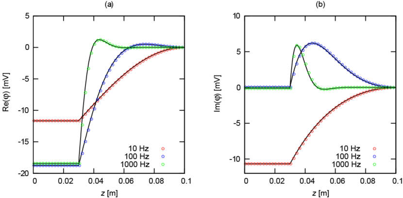
Figure 2: Comparison between (a) the real and (b) the imaginary parts of the electrical potential of a rock sample containing a horizontal layer at its center based on the analytical solution derived in this study (solid lines) and the numerical framework by Jougnot et al. (2013) (circles) as functions of position. The different curves correspond to three different frequencies of the applied harmonic compression. The imaginary part is related to the lag between the applied oscillatory compression and the resulting electrical potential distribution.

We first consider a rock sample with a vertical sidelength of 20 cm composed of a stiff, low-permeability host rock with a porosity of 0.05 (material 1 in Table 1), permeated at its center by a compliant, high-permeability horizontal layer with a thickness of 6 cm and a porosity of 0.4 (material 3 in Table 1). The sample is subjected to a harmonic compression of amplitude $\Delta P=1\ \text{kPa}$ and frequencies ranging from 1 to 10⁴ Hz. Before analyzing the seismoelectric response of this sample, we show in Fig. 2 a comparison between the electrical potential calculated with the analytical solution described in this work and the solution obtained using the numerical framework proposed by Jougnot et al. (2013). Due to the symmetry of the solution, we only show the response in the upper half of the sample. We observe excellent agreement between the electrical potential curves obtained using the analytical and numerical methodologies.

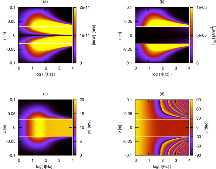
Figure 3: (a) Relative fluid velocity, (b) electrical source current density, and (c) amplitude and (d) phase of the electrical potential corresponding to a rectangular, stiff, low-permeability host rock containing a compliant, high-permeability horizontal layer at its center. The porosity of the layer is 0.4 (material 3 in Table 1), whereas that of the host rock is 0.05 (material 1 in Table 1). In all cases, the panels show the parameters along the $z$-axis as functions of the frequency of the applied harmonic compression. For visualization purposes, we indicate the boundaries of the layer using white lines.

Returning to the analytical solution for the compliant layer, Fig. 3(a) shows the amplitude of the resulting relative fluid velocity along the $z$-axis of the sample as a function of frequency. Due to the strong contrast between the compressibilities of the two materials, significant relative fluid velocities arise in both the host rock and the layer. There is a frequency at which the spatial extension of host rock affected by fluid flow is at its maximum, which we denote as the peak frequency. The characteristic frequency $f_{c}$ given by Eq. (15) is indicative of this frequency, since for such a value the diffusion length in the host rock is comparable to the characteristic size of the region. For lower frequencies, fluid velocities tend to become negligible. For higher frequencies, the regions of the host rock affected by fluid flow tend to only include the immediate vicinity of the boundaries of the layer, but the magnitude of the relative fluid velocity is important and increases with frequency. Relative fluid velocity is also important inside the layer, mainly in the vicinity of the boundaries. Since the permeability of this material is much higher, the corresponding peak frequency occurs at higher frequencies, as suggested by Eq. (13) and (15).

A significant current density (Fig. 3(b)) prevails in the host rock due to the relative fluid velocity field (Fig. 3(a)) produced by the compression. Moreover, the source current density clearly depends on the frequency, a relation that arises from the frequency-dependence of the induced fluid flow. The maximum current densities occur at the contacts between the two materials, where the relative fluid velocity is also maximum. Within the layer, even though significant fluid flow also takes place, the resulting source current density is very small, since the effective excess charge is much smaller in this material characterized by a much higher permeability (Table  1, Eq. (46)).

Significant electrical potential differences (Fig. 3(c)), well above the $\sim$ 0.01 mV threshold of laboratory experiments (e.g., Zhu & Toksöz, 2005; Schakel et al., 2012), arise in response to the oscillatory compression. These results are consistent with those of Jougnot et al. (2013) for fractured rocks and points to the importance of wave-induced fluid flow effects on seismoelectric signals in the presence of porosity variations. In the host rock, the frequency-dependence of the electrical potential distribution is very similar to that of the current density. Moreover, the region in the host rock characterized by significant values of electrical potential has its maximum spatial extension at the corresponding peak frequency. Inside the layer the behaviour is different. For each frequency, the amplitude of the electrical potential is rather constant. This happens because in this high-permeability material the effective excess charge is small while the electrical conductivity is large, which implies that the electrical potential is reduced to a near-constant value, $S_{1}$ (Eq. (35)). Because the electrical potential is continuous, this constant corresponds to the value of the electrical potential at the contact between the two materials.

The resulting electrical potential is not only characterized by its amplitude but also by its phase. For relatively low frequencies, the phase $\theta$ of the electrical potential remains constant, while for high frequencies it shows rapid changes within the host rock (Fig. 3(d)). Inside the layer $\theta$ remains constant, in agreement with the behaviour observed for the amplitude of the electrical potential in this region (Fig. 3(c)).

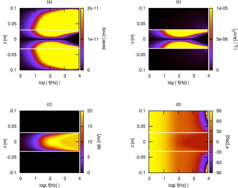
Figure 4: (a) Relative fluid velocity, (b) electrical source current density, and (c) amplitude and (d) phase of the electrical potential corresponding to a rectangular, compliant, high-permeability host rock containing a stiff, low-permeability horizontal layer at its center. The porosity of the layer is 0.05 (material 1 of Table 1), whereas that of the host rock is 0.4 (material 3 in Table 1). In all cases, the panels show the parameters along the $z$-axis and as functions of the frequency of the applied harmonic compression. For visualization purposes, we indicate the boundaries of the layer using white lines.

3.2.2 Stiff, low-permeability layer

We now repeat the preceding analysis, but with the properties of the host rock and of the layer interchanged. That is, we assume that the layer and the host rock have porosities of 0.05 (material 1) and 0.4 (material 3), respectively, with the corresponding petrophysical properties given in Table 1. Due to the strong compressibility contrast between the two materials, significant fluid flow arises in the vicinity of the contact zones between the host rock and the layer (Fig. 4(a)). Moreover, we observe that the peak frequency corresponding to the stiff, low-permeability material is higher compared with the previous situation (Fig. 3(a)). The reason for this is that the thickness of the stiff material is now smaller and, therefore, as dictated by Eq. (15), the characteristic frequency shifts towards higher frequencies compared to the situation depicted in Fig. 3(a). We also observe that for lower frequencies the fluid velocities tend to be negligible. For higher frequencies, significant fluid velocities prevail in smaller spatial extensions of the layer but their magnitudes increase with frequency. In the compliant host rock, the peak frequency is higher because this material is much more permeable (Eq. (15)), which explains the differing behaviour of the fluid velocity as compared with that observed in the stiff material.

The highest magnitudes of the electrical source current density are now concentrated inside the low permeability layer (Fig. 4(b)), which is characterized by high effective excess charges. As a result, and due to the imposed boundary conditions, when the layer is much stiffer and less permeable than the host rock, the electrical potential has a significant amplitude only inside the layer (Fig. 4(c)). Moreover, the electrical potential amplitude is frequency dependent, with a maximum at the centre of the layer and for a frequency close to the peak frequency (Fig. 4(a)). With respect to the phase of the electrical potential, significant phase changes within the sample take place at very high frequencies and in the host rock (Fig. 4(d)).

3.2.3 Sensitivity to the thickness of the layer

Figure 5: Electrical potential amplitude $|\varphi|$ for a layer having a thickness of $2L_{1}=$ 12 cm, that is, twice the value considered in the cases shown in Figs. 3 and 4. Panel (a) corresponds to a compliant, high-permeability layer (material 3 in Table 1) embedded in a stiff, low-permeability host rock (material 1 in Table 1), whereas panel (b) shows the results obtained when the two materials are interchanged. For visualization purposes, we indicate the boundaries of the layer using white lines.

To analyze the role played by the thickness of the layer, we now consider $2L_{1}=$ 12 cm for this region, that is, twice the original value, but leave the overall model setup and total thickness of the sample otherwise unchanged. The frequency- and space-dependence as well as the magnitude of the electrical potential for the compliant and stiff layer models, shown in Figs. 5(a) and  5(b), are similar to the ones shown in Figs. 3(c) and  4(c), respectively. However, the maxima of the electrical potential do not occur at the same frequencies. This shift in frequency can be explained by the dependence of the characteristic frequency $f_{c}$, which indicates the frequency at which maximum penetration of fluid flow takes place, on the characteristic size of the involved medium. Indeed, Eq. (15) dictates that $f_{c}$ is inversely proportional to the characteristic size of the region where fluid flow occurs. When the layer is more compliant and permeable than the host rock, the electrical potential is mainly produced by fluid flow in the host rock. As the thickness of the layer increases with respect to the situation depicted in Fig. 3(c), the characteristic size of the host rock is reduced. This reduction, in turn, produces an increase of the characteristic frequency $f_{c}$, which can be verified by comparing the frequency ranges where maximum electrical potential occurs in Fig. 3(c) and Fig. 5(a). Conversely, when the layer is stiffer and less permeable than the host rock, the electrical potential is produced by fluid flow inside the layer. Therefore, as the thickness of this region increases in the situation shown in Fig. 5(b), the characteristic frequency $f_{c}$ is reduced, in agreement with Eq. (15). Correspondingly, the frequency range where the electrical potential is maximum shifts towards lower frequencies, as can be verified by comparing Fig. 4(c) and Fig. 5(b). This result therefore indicates that the seismoelectric signal is sensitive to the layer thickness, which largely controls the frequency range where the maximum signal occurs.

3.2.4 Sensitivity to the compressibility contrast between layer and host rock

Figure 6: Electrical potential amplitude $|\varphi|$ for a rock sample containing a horizontal layer of thickness $2L_{1}=12~{}$cm and characterized by a reduced porosity contrast as compared with the situation depicted in Fig. 5. Panel (a) corresponds to porosity values of 0.2 (material 2 in Table 1) and 0.05 (material 1 in Table 1) for the layer and host rock, respectively, whereas panel (b) shows the results obtained when the two materials are interchanged. For visualization purposes, we indicate the boundaries of the layer using white lines.

Since the amount of fluid flow scales with the compressibility contrast between background and heterogeneities (e.g., Müller et al., 2010), the porosity contrast between the layer and the host rock is expected to have a major influence in the resulting seismoelectric response. To analyze this, we present in Fig. 6 the amplitude of the electrical potential as a function of frequency and space for the same geometries used in the cases shown in Fig. 5 but considering a reduced porosity contrast. We now use porosities of 0.05 (material 1 in Table 1) and 0.2 (material 2 in Table 1) for the stiff and compliant materials, respectively. By comparing Figs. 5 and Fig. 6, we can verify that the considered change in porosity contrast does not significantly affect the general frequency-dependence and spatial distribution of the electrical potential. This is because the geometry as well as the properties of the stiff material, which is the region where most of the current density arises, are similar. Conversely, there is an important decrease of the amplitude of the electrical potential. This effect is expected, as a reduction of porosity contrast implies a decrease of compressibility contrast. The latter causes a reduction of the wave-induced fluid flow (e.g., Müller et al., 2010) and, thus, of the source current density. These results illustrate that the magnitude of the electrical potential may contain information on the compressibility contrast between the layer and the host rock.

3.2.5 Asymptotic analysis

The previous parametric analysis suggests that key mechanical, structural and hydraulic properties of the central layer and of the host rock affect the seismoelectric response. In particular, while the compressibility contrast between the materials controls the magnitude of the resulting seismoelectric signal, the thickness and the permeability of the less permeable region determine the frequency range at which the response takes its maximum value.

In order to provide a formal description of this dependence and to further explore the analytical expression given by Eq. (35), we develop the low- and high-frequency asymptotic behaviors of the solution. Since from the previous analysis we conclude that, for a given frequency, the electrical potential is at its maximum at $z=0$, we derive these limits at this particular place of the sample. In Appendix B, we show that the low-frequency asymptote of the electrical potential at the center of the sample is given by

$$\varphi^{LF}_{z=0}(\omega)=\frac{i\omega\Delta P}{2}\left(\beta_{1}-\beta_{2}\right)\frac{\sum_{j=1}^{2}\frac{\bar{Q}_{v,j}^{\text{eff}}L_{j}}{\sigma_{j}}}{\sum_{j=1}^{2}\frac{N_{j}}{L_{j}}},$$ (47)

whereas the high-frequency asymptote is

$$\varphi^{HF}_{z=0}(\omega)=-\Delta P\left(\beta_{1}-\beta_{2}\right)\frac{\sum_{j=1}^{2}\frac{\bar{Q}_{v,j}^{\text{eff}}}{\sigma_{j}}\sqrt{\kappa_{j}N_{j}}}{\sum_{j=1}^{2}\sqrt{\frac{N_{j}}{\kappa_{j}}}}.$$ (48)

The latter expression is the high-frequency limit of the solution obtained based on the premise that frequency is lower than Biot’s critical frequency. In other words, Eq. (48) represents the high-frequency limit of the low-frequency-domain solution.

Figure 7 shows the amplitude of the electrical potential at the center of the sample as a function of frequency, for both the compliant- and stiff-layer cases considered in Figs. 3 and 4, together with the corresponding low- and high-frequency asymptotes. There is very good agreement between the general solutions and the low- and high-frequency asymptotes. Moreover, this analysis shows the importance of the analytical solutions obtained in this work and, in particular, of these asymptotes, since they allow us to explicitly observe how the various petrophysical parameters contribute to the seismoelectric response. The high-frequency asymptote, which is constant, can be considered as an indicator of the maximum magnitude of the electrical potential. Therefore, Eq. (48) allows for a direct appreciation of how the different petrophysical properties control the amplitude of the seismoelectric response. This maximum amplitude is directly proportional to the applied stress, to a weighted average of the effective excess charges of the two media, and to the Skempton coefficient contrast between the host rock and the layer. The Skempton coefficient is the ratio of the fluid pressure increase to the corresponding applied stress for undrained conditions (e.g., Wang, 2000). Correspondingly, the term

$$\Delta P\left(\beta_{1}-\beta_{2}\right),$$ (49)

appearing in Eq. (48) constitutes a measure of the fluid pressure gradient induced across the interfaces separating the host rock and the layer. It is thus reasonable that the maximum amplitude of the seismoelectric response turns out to be directly proportional to this parameter, since the fluid pressure gradient induced by the applied compression triggers the fluid flow and the corresponding seismoelectric signal.

Employing Eq. (46), the weighted average of the effective excess charges included in Eq. (48) satisfies

$$\frac{\sum_{j=1}^{2}\frac{\bar{Q}_{v,j}^{\text{eff}}}{\sigma_{j}}\sqrt{\kappa_{j}N_{j}}}{\sum_{j=1}^{2}\sqrt{\frac{N_{j}}{\kappa_{j}}}}\propto\frac{\sum_{j=1}^{2}\frac{\kappa_{j}^{-0.32}\sqrt{N_{j}}}{\sigma_{j}}}{\sum_{j=1}^{2}\sqrt{\frac{N_{j}}{\kappa_{j}}}}.$$ (50)

If the permeability contrast between the two media is strong, the numerator and denominator of the right-hand side of Eq. (50) are controlled by the term corresponding to the material of lower permeability, that is,

$$\frac{\sum_{j=1}^{2}\frac{\bar{Q}_{v,j}^{\text{eff}}}{\sigma_{j}}\sqrt{\kappa_{j}N_{j}}}{\sum_{j=1}^{2}\sqrt{\frac{N_{j}}{\kappa_{j}}}}\propto\frac{\kappa_{min}^{-0.32}\sqrt{N_{min}}}{\sqrt{\frac{N_{min}}{\kappa_{min}}}}=\kappa_{min}^{0.18},$$ (51)

where the subscript $min$ denotes the material with the lowest permeability. Substituting this relation into Eq. (48), we obtain

$$\varphi^{HF}(\omega)\propto-\Delta P\left(\beta_{1}-\beta_{2}\right)\kappa_{min}^{0.18}.$$ (52)

Equation (52) suggests that the magnitude of the resulting electrical potential, in the case of strong permeability contrasts, is directly proportional to $\kappa_{min}^{0.18}$. This result also indicates that the hydraulic properties of the most permeable material and the thicknesses of the layer and of the host rock do not affect the magnitude of the seismoelectric response. This is in agreement with the results presented in this work, where similar values for the maximum amplitudes of the electrical potential were found when the materials of the host rock and the layer were interchanged.

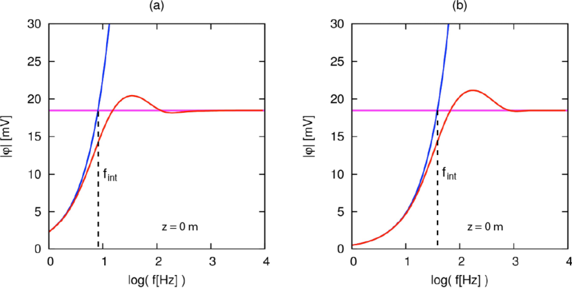
Figure 7: Amplitude of the electrical potential in the center of the sample ($z=0$) as a function of frequency. Panel (a) corresponds to porosity values of 0.4 (material 3 in Table 1) and 0.05 (material 1 in Table 1) for the layer and host rock, respectively, whereas panel (b) shows the results obtained when the two materials are interchanged. Red lines correspond to the exact solution (Eq. (35)), the blue ones to their low-frequency asymptotic solution (Eq. (47)) and the pink ones to their high-frequency asymptotic solution (Eq. (48)).

The frequency at which the low- and high-frequency asymptotes intercepts, $f_{int}$, can be used as an indicator of the frequency at which the electrical potential reaches its peak. This intersection can differ with respect to the true peak frequency by almost one order-of-magnitude (Fig. 7). However, its dependence on the mechanical, hydraulic, and structural properties of the heterogeneous sample are expected to also hold in the case of the true peak frequency. By requiring equality of Eqs. (47) and (48), $f_{int}$ can be defined as

$$f_{int}=\frac{1}{2\pi}\frac{\sum_{j=1}^{2}\frac{\bar{Q}_{v,j}^{\text{eff}}}{\sigma_{j}}\sqrt{\kappa_{j}N_{j}}}{\sum_{j=1}^{2}\sqrt{\frac{N_{j}}{\kappa_{j}}}}\frac{\sum_{j=1}^{2}\frac{N_{j}}{L_{j}}}{\sum_{j=1}^{2}\frac{\bar{Q}_{v,j}^{\text{eff}}L_{j}}{\sigma_{j}}}.$$ (53)

Hence, the frequency of the peak of the electrical potential does not depend on the amplitude of the applied pressure, $\Delta P$. Interestingly, it does not depend on the Skempton coefficient contrast of the materials either.

Considering the case of strong permeability contrasts and using Eq. (52) instead of Eq. (48) to obtain $f_{int}$, yields

$$f_{int}\propto\frac{\kappa_{min}}{L_{min}}\sum_{j=1}^{2}\frac{N_{j}}{L_{j}}.$$ (54)

This equation shows that the frequency of the peak of the electrical potential is directly proportional to $\kappa_{min}$, whereas the hydraulic properties of the most permeable regions do not affect this parameter. In addition, the structural characteristics of the sample do affect the location of the peak, which is inversely proportional to the thickness of the less permeable material. Also, the mechanical properties, scaled by the thicknesses of the corresponding layers, affect the peak frequency.

3.3 Analysis of fractured media

Fractures are usually composed of very compliant material and the resulting strong compressibility contrast with respect to the host rock is expected to favor particularly strong seismoelectric signals in response to the application of oscillatory compressions (Jougnot et al., 2013). In order to explore this in more detail, we estimate the seismoelectric responses of fractured media by making use of the model developed in Section 2.3. According to this model, in which the aperture of the fracture is considered negligible, the seismoelectric response is controlled by the properties of the host rock, the size of the sample, and the compliance of the fracture. The latter is represented by the drained normal compliance $Z_{N}$ (Eq. (39)).

To study the behaviour of the seismoelectric response for different characteristics of fracture and host rock materials, we consider a rectangular rock sample with vertical sidelength of 20 cm containing a horizontal fracture at its center. As in the previous analysis, the sample is subjected to a harmonic compression with an amplitude $\Delta P=1$ kPa and frequencies ranging from 1 to 10⁴ Hz. For the host rock, we consider a sandstone with a porosity of 0.05 (material 1 in Table 1), while, as proposed by Nakagawa & Schoenberg (2007), we use a drained normal compliance $Z_{N}=10^{-8}~{}\text{m kPa}^{-1}$ for the fracture. Very strong electrical potential differences, that could be measured using standard laboratory techniques, arise in response to the applied oscillatory compression (Fig. 8(a)). Moreover, the overall frequency- and space-dependence characteristics of the electrical potential are essentially the same as in the case of a rock sample containing a horizontal compliant and permeable layer. Indeed, there is also a frequency range at which both the magnitude and the spatial extension of the electrical potential are at a maximum.

Figure 8: Absolute value of the electrical potential $|\varphi|$ along the $z$-axis as a function of frequency for samples containing a horizontal fracture at their centers. Panel (a) corresponds to a host rock with a porosity $\phi$ of $0.05$ (material 1 in Table 1) and a fracture drained normal compliance $Z_{N}$ of $10^{-8}\text{m kPa}^{-1}$; in panel (b) $\phi=0.4$ (material 3 in Table 1) and $Z_{N}=10^{-8}\text{m kPa}^{-1}$; in panel (c) $\phi=0.05$ and $Z_{N}=10^{-6}\text{m kPa}^{-1}$, and in panel (d) $\phi=0.4$ and $Z_{N}=10^{-6}\text{m kPa}^{-1}$.

To study the role played by the characteristics of the host rock, we change its properties to those of a sandstone with a porosity of 0.4 (material 3 in Table 1). The corresponding increases of the permeability and of the compressibility of the host rock produce significant changes in the resulting electrical potential (Fig. 8(b)). Indeed, the magnitude of the signal is significantly smaller than that shown in Fig. 8(a), which was evaluated using smaller values of permeability and compressibility of the host rock. This, in turn, indicates that, according to Eq. (52), the effect related to the reduction of compressibility contrast between fracture and host rock overcomes that related to the increase of the permeability of the host rock. In addition, as suggested by Eq. (54), the increase of the host rock permeability shifts the frequency range where the maximum value and maximum spatial penetration of the electrical signal occur towards higher values.

The compliance of the fracture, represented by $Z_{N}$, controls the compressibility contrast with regard to the host rock. This parameter is thus expected to play a major role in the seismoelectric response of fractured materials. To verify this, we show in Fig. 8(c) the electrical potential for a fractured sample having a host rock porosity of 0.05, that is, the same value employed to calculate the electrical potential represented in Fig. 8(a), but with a drained normal compliance $Z_{N}=10^{-6}$ m kPa^-1. The comparison between Figs. 8(a) and  8(c) shows that the overall frequency-dependence and spatial distribution of the electrical potential are very similar. However, an increase of fracture drained normal compliance implies an increase of compressibility contrast between fracture and host rock. This results in a significantly larger magnitude of the electrical potential.

Finally, Fig. 8(d) shows the amplitude of the electrical potential for a host rock corresponding to a sandstone with a porosity of 0.4 and a fracture with a drained normal compliance $Z_{N}=10^{-6}\text{m kPa}^{-1}$. By comparing this electrical potential with the one represented in Fig.  8(a), we see a significant reduction of the magnitude of the signal together with a shift towards higher values of the peak frequency. The reduction in magnitude indicates that the increase of host rock compressibility related to the porosity change affects the compressibility contrast more significantly than the increase of compliance of the fracture. In addition, as dictated by Eq. (54), the increase of host rock permeability related to the porosity variation shifts towards higher values the peak frequency of the electrical potential.

4 Discussion

In accordance with Jougnot et al. (2013), our results indicate that seismoelectric signals are highly sensitive to the presence of mesoscopic heterogeneities. The analytical solutions obtained in this work provide the explicit dependence of these signals on the structural, mechanical and hydraulic properties of the materials involved. In the following, we discuss some of the implications of this dependence.

Assuming a laboratory experiment where electrodes are placed vertically along the sample shown in Fig. 1, our results suggest that one could identify the presence of a compliant and permeable layer as the region where the amplitude of the electrical potential remains constant, and of a stiff and less permeable layer as the region exhibiting a significant electrical potential gradient. Alternatively, the center of the layer can be identified by finding the position of the maximum amplitude of the potential. In the case of fractured rocks, the drained normal compliance $Z_{N}$ is a parameter of key importance for simulating seismic wave propagation in the framework of the linear slip theory (e.g., Schoenberg, 1980), but it is often poorly constrained. Our analytical solution for the seismoelectric response of a fractured rock could conceivably be employed to estimate the drained normal compliance of a fracture based on electrical potential measurements. First, the position of the fracture could be identified as the region where the maximum amplitude is measured and, then, the drained normal compliance could be estimated by inserting the measured value of electrical potential in Eq. (40). Additionally, the permeability of the host rock could also be retrieved, provided that measurements are made at several distances from the fracture or at different frequencies.

The present analysis considers a rock sample subjected to an oscillatory compressibility test, which allows us to explore seismoelectric signals related to the generation of Biot’s slow waves at interfaces separating layers with differing mechanical properties. These results have interesting implications related to seismic wave propagation. The seismoelectric signals are expected to decay as the amplitude of the seismic wave progressively diminishes due to geometrical divergence, scattering, and attenuation effects. Therefore, in the case of a compressional seismic wave propagating through a periodic 1D medium composed of an assembly of the sample shown in Fig. 1, similar to the situation studied by White et al. (1975) in the context of seismic attenuation due to wave-induced fluid flow, the electrical-potential contribution is expected to be similar to that shown in this work, but scaled according to the local stress applied by the passing seismic wave. A complete extension of the methodology presented in this work to seismic wave propagation is, however, not straightforward. In addition to scattering and amplitude distortion effects, further contributions, such as the effects of wavelength-scale relative fluid flow produced by the seismic wave, should be taken into account. The analysis of numerical simulations of seismic wave propagation through porous media containing mesoscopic heterogeneities and of the resulting seismoelectric responses will be the subject of forthcoming studies.

Among the implications of the explicit dependence of the electrical potential on rock parameters presented in this work, it is interesting to highlight that the magnitude of the resulting signal is directly proportional to the Skempton coefficient contrast between the involved materials, to the amplitude of the applied compression and, in the case of strong permeability contrasts, it is also highly influenced by the permeability of the less permeable material. In such a situation the peak frequency of the electrical potential is largely governed by the permeability and the thickness of the region containing the less permeable material. Any attempt to model the coherent noise observed in seismoelectric signals arising potentially from mesoscopic heterogeneities, as suggested by Jougnot et al. (2013), should carefully constrain the values of these parameters. Conversely, in the case of strong permeability contrasts the hydraulic and electrical properties of the most permeable material do not need to be determined with high precision, as the seismoelectric signals turned out to be virtually insensitive to these parameters.

5 Conclusions

We have derived an analytical solution that describes the seismoelectric response of a rectangular rock sample containing a horizontal layer at its center that is subjected to an oscillatory compressibility experiment. The resulting solution was also adapted to compute the seismoelectric response of a rock sample containing a horizontal fracture at its center.

The seismoelectric responses predicted by the analytical solutions were explored and allowed us to shed some light into their dependence on mechanical, hydraulic, and structural properties of the host rock and the layer or fracture. As a general result, we found that the seismoelectric signals produced by oscillatory compressibility tests could be measured in standard laboratory experiments. The significant amplitudes of the seismoelectric signals point to the importance of considering mesoscopic effects when employing the seismoelectic method. Moreover, the analysis indicated that the maximum amplitude of the electrical potential is directly proportional to the applied stress, to the Skempton coefficient contrast between the host rock and the heterogeneity, and to a weighted average of the effective excess charge of the two materials. In presence of strong permeability variations we found that this weighted average is mainly controlled by the permeability of the less permeable material and that the frequency at which the maximum electrical potential prevails is governed by the permeability and thickness of the region containing such material.

Although the analytical solutions considered in this work are based on simple 1D models, they constitute useful tools for exploring the details of the physical processes involved in the seismoelectric method in presence of mesoscopic heterogeneities. Moreover, they may open the possibility of retrieving key rock properties, such as permeability and fracture drained normal compliance, from seismoelectric measurements.

Appendix A 1D Skempton coefficient

The Skempton coefficient is defined as the ratio between the induced fluid pressure increase to the applied stress for undrained conditions (e.g., Wang, 2000)

$$\beta\equiv-\frac{\delta p_{f}}{\delta\tau}\Big{|}_{\zeta=0},$$ (55)

where $\zeta$ is the increment of fluid content, which in 1D is given by $\zeta\equiv-\partial w/\partial z$. This parameter measures how the applied stress is distributed between the solid frame and the pore fluid (Wang, 2000).

Imposing the undrained condition $\zeta=0$ in Eqs. (4) and (5), we get

$$\tau=H\frac{\partial u}{\partial z},$$ (56)

$$p_{f}=-\alpha M\frac{\partial u}{\partial z}.$$ (57)

The 1D Skempton coefficient is thus obtained by taking the ratio between Eqs. (56) and (57)

$$\beta=\frac{\alpha M}{H}.$$ (58)

Appendix B Asymptotic analysis of the electrical potential at the center of the sample

Equation (35), together with the Eqs. (36) and (37), constitute an analytical model for describing the seismoelectric response of a rock sample containing a horizontal layer that is subjected to an oscillatory compressibility test. Now we focus on the values of $\varphi(z)$ at $z=0$, that is, at the center of the sample. From Eq. (35), we get for the electrical potential

$$\varphi(0)=-2\frac{i\omega\bar{Q}_{v,1}^{\text{eff}}}{\sigma_{1}}\frac{A_{1}}{k_{1}}+S_{1}.$$ (59)

Replacing the corresponding expressions for $A_{1}$ and $S_{1}$ (Eqs. (26) and (36) respectively) in (59) we obtain

$$\varphi(0)=\frac{i\omega\Delta P\left(\beta_{1}-\beta_{2}\right)\sum_{j=1}^{2}\frac{\bar{Q}_{v,j}^{\text{eff}}}{\sigma_{j}k_{j}}\left[\frac{1-cosh(k_{j}L_{j})}{sinh(k_{j}L_{j})}\right]}{\sum_{j=1}^{2}N_{j}k_{j}\ coth(k_{j}L_{j})}.$$ (60)

This equation predicts that the amplitude of the electrical potential is proportional to the Skempton coefficient contrast of the two involved materials and to the amplitude of the applied compression. However, the dependence of $\varphi(0)$ on $\bar{Q}_{v,j}^{\text{eff}}$, $\sigma_{j}$ and $L_{j}$ and $\kappa_{j}$ is not straightforward because of the hyperbolic functions involved. Developing the low- and high-frequency asymptotes of this equation may help understand the roles played by the different mechanical, hydraulic and structural properties on the seismoelectric response.

B.1 Low-frequency asymptote

Using first-order Taylor expansions the following approximations can be obtained

$$\frac{1-cosh(k_{j}L_{j})}{sinh(k_{j}L_{j})}\simeq k_{j}L_{j},$$ (61)

$$k_{j}L_{j}\ coth(k_{j}L_{j})\simeq 1.$$ (62)

Eqs. (61) and (62) are good approximations when $k_{j}L_{j}\rightarrow 0$, which occurs when $\omega\rightarrow 0$. Replacing these first-order approximations in Eq. (60), we get the low-frequency asymptote for the electrical potential in the center of the sample

$$\varphi^{LF}_{z=0}(\omega)=\frac{\frac{i\omega\Delta P}{2}\left(\beta_{1}-\beta_{2}\right)\sum_{j=1}^{2}\frac{\bar{Q}_{v,j}^{\text{eff}}L_{j}}{\sigma_{j}}}{\sum_{j=1}^{2}\frac{N_{j}}{L_{j}}}.$$ (63)

B.2 High-frequency asymptote

In order to explore the high-frequency behaviour of $\varphi(0)$, we use the following approximations which are valid when $k_{j}L_{j}\rightarrow\infty$

$$\frac{1-cosh(k_{j}L_{j})}{sinh(k_{j}L_{j})}\simeq-1,$$ (64)

$$coth(k_{j}L_{j})\simeq 1.$$ (65)

Replacing these expressions in (60) we obtain for the high-frequency asymptote

$$\varphi^{HF}_{z=0}(\omega)=\frac{-i\omega\Delta P\left(\beta_{1}-\beta_{2}\right)\sum_{j=1}^{2}\frac{\bar{Q}_{v,j}^{\text{eff}}}{\sigma_{j}k_{j}}}{\sum_{j=1}^{2}N_{j}k_{j}}.$$ (66)

The expression for $k_{j}$ as a function of $\omega$ can be obtained by combining Eqs.(13), (14) and (17)

$$k_{j}=\sqrt{\frac{i\omega\eta}{\kappa_{j}N_{j}}}.$$ (67)

Then, replacing (67) in (66) one obtains

$$\varphi^{HF}_{z=0}(\omega)=\frac{-\Delta P\left(\beta_{1}-\beta_{2}\right)\sum_{j=1}^{2}\frac{\bar{Q}_{v,j}^{\text{eff}}}{\sigma_{j}}\sqrt{\kappa_{j}N_{j}}}{\sum_{j=1}^{2}\sqrt{\frac{N_{j}}{\kappa_{j}}}}.$$ (68)

References

- Archie (1942) Archie, G., 1942. The electrical resistivity log as an aid in determining some reservoir characteristics, Transaction of the American Institute of Mining and Metallurgical Engineers, 146, 54–61.
- Biot (1941) Biot, M., 1941. General theory of three-dimensional consolidation, Journal of Applied Physics, 12, 155–164.
- Biot (1956a) Biot, M., 1956a. Theory of propagation of elastic waves in a fluid saturated porous solid. II. Higher frequency range, Journal of the Acoustical Society of America, 28, 179–191.
- Biot (1956b) Biot, M., 1956b. Theory of propagation of elastic waves in a fluid saturated porous solid. I. Low frequency range, Journal of the Acoustical Society of America, 28, 168–178.
- Biot (1962) Biot, M., 1962. Mechanics of deformation and acoustic propagation in porous media, Journal of Applied Physics, 33, 1482–1498.
- Brajanovski et al. (2005) Brajanovski, M., Gurevich, B., & Schoenberg, M., 2005. A model for P-wave attenuation and dispersion in a porous medium permeated by aligned fractures, Geophysical Journal International, 163, 372–384.
- Guan & Hu (2008) Guan, W. & Hu, H., 2008. Finite-difference modeling of the electroseismic logging in a fluid-saturated porous formation, Journal of Computational Physics, 227(11), 5633–5648.
- Haartsen & Pride (1997) Haartsen, M. & Pride, S., 1997. Electroseismic waves from point sources in layered media, Journal of Geophysical Research, 102, 24,745–24,769.
- Haines & Pride (2006) Haines, S. S. & Pride, S. R., 2006. Seismoelectric numerical modeling on a grid, Geophysics, 71(6), N57–N65.
- Hunter (1981) Hunter, R., 1981. Zeta Potential in Colloid Science: Principles and Applications, Colloid Science Series, Academic Press.
- Jardani et al. (2007) Jardani, A., Revil, A., Bolève, A., Crespy, A., Dupont, J., Barrash, W., & Malama, B., 2007. Tomography of the Darcy velocity from self-potential measurements, Geophysical Research Letters, 34(24), L24403.
- Jardani et al. (2010) Jardani, A., Revil, A., Slob, E., & Sölner, W., 2010. Stochastic joint inversion of 2D sesimic and seismoelectric signals in linear poroelastic materials: A numerical investigation, Geophysics, 34(75), N19–N31.
- Jougnot et al. (2012) Jougnot, D., Linde, N., Revil, A., & Doussan, C., 2012. Derivation of soil-specific streaming potential electrical parameters from hydrodynamic characteristics of partially saturated soils, Vadose Zone Journal, 11(1).
- Jougnot et al. (2013) Jougnot, D., Rubino, J. G., Rosas Carbajal, M., Linde, N., & Holliger, K., 2013. Seismoelectric effects due to mesoscopic heterogeneities, Geophysical Research Letters, 40, 2033—2037.
- Jouniaux (2011) Jouniaux, L., 2011. Hydraulic Conductivity - Issues, Determination and Applications, chap. Electrokinetic techniques for the determination of hydraulic conductivity, InTech Publisher.
- Jouniaux & Pozzi (1995) Jouniaux, L. & Pozzi, J.-P., 1995. Streaming potential and permeability of saturated sandstones under triaxial stress: Consequences for electrotelluric anomalies prior to earthquakes, Journal of Geophysical Research, 100(B6), 10197–10209.
- Krief et al. (1990) Krief, M., Garat, J., Stellingwerff, J., & Ventre, J., 1990. A petrophysical interpretation using the velocities of P and S waves (full waveform inversion), The Log Analyst, 31, 355–369.
- Mavko et al. (2009) Mavko, G., Mukerji, E., & Dvorkin, J., 2009. The Rock Physics Handbook: Tools for Seismic Analysis of Porous Media, Cambridge Univ. Press, New York, 524pp., 2nd edn.
- Müller et al. (2010) Müller, T., Gurevich, B., & Lebedev, M., 2010. Seismic wave attenuation and dispersion resulting from wave-induced flow in porous rocks - A review, Geophysics, 75, 75A147–75A164.
- Nakagawa & Schoenberg (2007) Nakagawa, S. & Schoenberg, M., 2007. Poroelastic modeling of seismic boundary conditions across a fracture, Journal of the Acoustical Society of America, 122, 831–847.
- Pride (1994) Pride, S., 1994. Governing equations for the coupled electromagnetics and acoustics of porous media, Physical Review B, 50, 15678–15696.
- Pride & Garambois (2002) Pride, S. & Garambois, S., 2002. The role of Biot slow waves in electroseismic wave phenomena, Journal of the Acoustical Society of America, 111, 697–706.
- Pride & Haartsen (1996) Pride, S. & Haartsen, M., 1996. Electroseismic wave properties, Journal of the Acoustical Society of America, 100, 1301–1315.
- Revil & Leroy (2004) Revil, A. & Leroy, P., 2004. Constitutive equations for ionic transport in porous shales, Journal of Geophysical Research, 109(B3), B03208.
- Revil & Mahardika (2013) Revil, A. & Mahardika, H., 2013. Coupled hydromechanical and electromagnetic disturbances in unsaturated porous materials, Water Resources Research, 49(2), 744–766.
- Rubino et al. (2009) Rubino, J. G., Ravazzoli, C. L., & Santos, J. E., 2009. Equivalent viscoelastic solids for heterogeneous fluid-saturated porous rocks, Geophysics, 74, N1–N13.
- Rubino et al. (2013) Rubino, J. G., Monachesi, L. B., Müller, T. M., Guarracino, L., & Holliger, K., 2013. Seismic wave attenuation and dispersion due to wave-induced fluid flow in rocks with strong permeability fluctuations, Journal of the Acoustical Society of America, 134, 4742–4751.
- Schakel et al. (2012) Schakel, M., Smeulders, D., Slob, E., & Heller, H., 2012. Seismoelectric fluid/porous-medium interface response model and measurements, Transport in Porous Media, 93(2), 271–282.
- Schoenberg (1980) Schoenberg, M., 1980. Elastic wave behavior across linear slip interfaces, Journal of the Acoustical Society of America, 68, 1516–1521.
- Sill (1983) Sill, W., 1983. Self-potential modeling from primary flows, Geophysics, 48(1), 76–86.
- Suski et al. (2006) Suski, B., Revil, A., Titov, K., Konosavsky, P., Voltz, M., Dagès, C., & Huttel, O., 2006. Monitoring of an infiltration experiment using the self-potential method, Water Resources Research, 42(8), W08418.
- Tardif et al. (2011) Tardif, E., Glover, P. W., & Ruel, J., 2011. Frequency-dependent streaming potential of Ottawa sand, Journal of Geophysical Research, 116(B4).
- Thompson & Gist (1993) Thompson, A. & Gist, G., 1993. Geophysical applications of electrokinetic conversion, The Leading Edge, 12, 1169–1173.
- Tisato & Quintal (2013) Tisato, N. & Quintal, B., 2013. Measurements of seismic attenuation and transient fluid pressure in partially saturated Berea sandstone: evidence of fluid flow on the mesoscopic scaleberea sandstone: evidence of fluid flow on the mesoscopic scale, Geophysical Journal International, 195(1), 342–351.
- Wang (2000) Wang, H. F., 2000. Theory of linear poroelasticity with applications to geomechanics and hydrogeology, Princeton University Press.
- White et al. (1975) White, J., Mikhaylova, N., & Lyakhovitskiy, F., 1975. Low-frequency seismic waves in fluid-saturated layered rocks, Izvestija Academy of Science USSR, Physics of the Solid Earth, 10, 654–659.
- Zhu & Toksöz (2005) Zhu, Z. & Toksöz, M., 2005. Seismoelectric and seismomagnetic measurements in fractured borehole models, Geophysics, 70(4), F45–F51.
- Zyserman et al. (2010) Zyserman, F. I., Gauzellino, P. M., & Santos, J. E., 2010. Finite element modeling of SHTE and PSVTM electroseismics, Journal of applied geophysics, 72(2), 79–91.