Statistics of heat exchange between two resistors

Abstract

We study energy flow between two resistors coupled by an arbitrary linear and lossless electric circuit. We show that the fluctuations of energy transferred between the resistors are determined by random scattering of photons on an effective barrier with frequency dependent transmission probability $\tau(\omega)$. We express the latter in terms of the circuit parameters. Our results are valid in both quantum and classical regimes and for non-equilibrium electron distribution functions in the resistors. Our theory is in good agreement with recent experiment performed in the classical regime.

I Introduction

The problem of energy exchange between two resistors has been first analyzed by Nyquist Nyquist on the way towards his famous formula for the current noise of a resistor,

$$S_{I}=4k_{B}T/R.$$ (1)

Here $S_{I}$ is the spectral density of noise at low frequencies $|\omega|\ll k_{B}T/\hbar$, $k_{B}$ is the Boltzmann constant, $T$ is the temperature and $R$ is the resistance. Equation (1) has been confirmed by Johnson Johnson and by numerous subsequent experiments. For a long time afterwards transport of heat in electric circuits has been considered well understood. Recently, however, it has attracted renewed attention due to advances both in theory and in technology. On the theoretical side, the discovery of the fluctuation theorem BK ; Evans ; Crooks ; Campisi has triggered the interest in the statistics of heat transport. Statistics of effective electron temperature fluctuations in small metallic grains is also under discussion Nazarov1 ; Nazarov2 . The experiments have recently advanced in two directions. First, quantum transport of heat between two resistors coupled by superconducting wires and separated by up to 50 $\mu$m distance has been demonstrated at sub-kelvin temperatures Meshke ; Timofeev . Second, utilizing low noise amplifiers Ciliberto et al. have recently measured the full statistical distribution of heat transferred between two resistors kept at temperatures 88 K and 296 K respectively Ciliberto1 ; Ciliberto2 . They have verified the validity of the fluctuation theorem and worked out a theoretical model based on Nyquist’s formula (1).

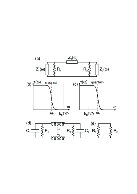
Figure 1: Two resistors connected in a linear circuit: (a) general case – resistors are connected by an arbitrary reactive element with the impedance $Z_{0}(\omega)$ and shunted by the reactive impedances $Z_{1}(\omega),Z_{2}(\omega)$; (b) classical regime $T_{1},T_{2}\gtrsim\omega_{c}$; (c) quantum regime $T_{1},T_{2}\lesssim\omega_{c}$; (d) realistic model, with stray capacitances $C_{1},C_{2}$ and wire inductances $L_{1},L_{2}$; (e) resistors directly coupled by two ideal zero resistance wires.

Motivated by these developments, in this letter we propose a theory of full counting statistics of photon mediated heat exchange between two metallic resistors valid both at high and at low temperatures, where the classical formula for the noise (1) can no longer be used. We consider two resistors, $R_{1}$ and $R_{2}$ shunted by impedances $Z_{1}(\omega)$ and $Z_{2}(\omega)$, and coupled by a linear element (e.g. transmission line, capacitor, etc.) having the impedance $Z_{0}(\omega)$ (see Fig. 1a). The impedances $Z_{j}(\omega)$, ($j=0,1,2$) are purely reactive and do not generate noise. The average photonic heat current flowing from the resistor 1 to the resistor 2 reads

$$J_{Q}=\int_{0}^{\infty}\frac{d\omega}{2\pi}\,\omega\tau(\omega)\big{[}n_{1}(\omega)-n_{2}(\omega)\big{]},$$ (2)

where $\tau(\omega)$ is the effective transmission, which we will specify later, $n_{j}(\omega)$ are photon distribution functions (here and below we put $k_{B}=\hbar=1$). Typically $\tau(\omega)$ drops at certain cutoff frequency $\omega_{c}$. Assuming that $n_{1}(\omega),n_{2}(\omega)$ have equilibrium Bose form with the temperatures $T_{1}$ and $T_{2}$, one finds that at high temperatures, $T_{1},T_{2}\gtrsim\omega_{c}$ (Fig. 1b), $J_{Q}\approx\tau(0)\omega_{c}(T_{1}-T_{2})$ in agreement with experimental findings of Refs. Ciliberto1 ; Ciliberto2 . In this classical regime Nyquist’s formula (1) may be used to derive the heat current. In this letter we will be mostly interested in the opposite, quantum, limit $T_{1},T_{2}\lesssim\omega_{c}$ (Fig. 1c), which is relevant for typical low temperature experiments Meshke ; Timofeev . Indeed, the cutoff frequency may be estimated as $\omega_{c}\sim\min\{{1/R_{j}C_{j},R_{j}/L_{j}}\}$, where $C_{j}\sim\epsilon\epsilon_{0}l$ are stray capacitances, $L_{j}\sim\mu_{0}l$ are inductances of the wires (Fig. 1d), $\epsilon_{0}$ and $\mu_{0}$ are vacuum permittivity and permeability, $\epsilon$ is the dielectric constant, and $l$ is the characteristic size of the sample. For the parameters of the low temperature experiments Meshke ; Timofeev , namely $T\sim 100$ mK, $R\sim 1$ k$\Omega$ and $l\sim 10$ $\mu$m, one finds $T/\omega_{c}\sim 10^{-3}\ll 1$. Thus the circuit is in the quantum regime. In contrast, for the experiments by Ciliberto et al Ciliberto1 ; Ciliberto2 with $T\sim 100$ K, $R=10$ M$\Omega$ and $l\sim 1$ cm one finds $T/\omega_{c}\sim 10^{10}\gg 1$, which corresponds to strongly classical regime.

II Model

Our goal is to find the distribution of the energy $Q$ transferred from the resistor 1 to the resistor 2 during the time $t$, which we denote as $P(t,Q)$. It is more convenient to work with the cumulant generating function (CGF), $F(t,\lambda)$, which depends on the counting field $\lambda$ and defined as

$$e^{F(t,\lambda)}=\int dQ\,e^{i\lambda Q}P(t,Q).$$ (3)

We describe the system by a Hamiltonian

$$\hat{H}=\hat{H}_{0}+\hat{H}_{\rm em}+\hat{H}_{\rm int},$$ (4)

where $\hat{H}_{0}=\sum_{k\sigma}\epsilon_{k}\hat{a}^{\dagger}_{k\sigma}\hat{a}_{k\sigma}$ is the Hamiltonian of non-interacting electrons moving in the combined potential of ion lattice and impurities, $\hat{a}_{k\sigma}$ is an annihilation operator of an electron in the eigenstate $|\psi_{k\sigma}\rangle$ ($\sigma$ is the spin index) and $\epsilon_{k}$ is the corresponding eigen-energy; $\hat{H}_{\rm em}=\int d^{3}{\bm{r}}(\hat{\bm{E}}^{2}+\hat{\bm{H}}^{2})/8\pi$ is the Hamiltonian of electro-magnetic field; $\hat{\bm{E}}$ and $\hat{\bm{H}}$ are the operators of the electric and magnetic fields respectively; $\hat{H}_{\rm int}=-\sum_{kn,\sigma}e\hat{V}_{kn}\hat{a}^{\dagger}_{k\sigma}\hat{a}_{n\sigma}$ is the interaction Hamiltonian; and $\hat{V}_{kn}=\langle\psi_{k}|\hat{V}(\bm{r})|\psi_{n}\rangle$ are the matrix elements of the electric potential operator between two eigenfunctions of the non-interacting electron Hamiltonian $\hat{H}_{0}$. The Hamiltonian $\hat{H}_{0}$ describes the two resistors, the wires connecting them and the leads attached to them if they present.

An important point is the definition of the transferred energy $Q$. Here we have in mind the detection scheme based on normal metal - superconductor tunnel junctions attached to the resistors Meshke ; Timofeev . Such a junction allows one to measure the effective temperature of a resistor or, more generally, the distribution function, $f(E,{\bm{r}})$, of electrons in it Pothier . The latter can be converted into the total electron energy of the resistor $j$ ($j=1,2$) as ${\cal E}_{j}=2\int_{\Omega_{j}}d^{3}{\bm{r}}\int dE\,E\nu_{j}(E)f(E,{\bm{r}})$ (here $\Omega_{j}$ in the volume of the resistor $j$ and $\nu_{j}(E)$ is the density of states). Within this approach it is natural to define the transferred energy as the drop in the electronic energy of the resistor 1 during the time $t$, $Q=-{\cal E}_{1}(t)+{\cal E}_{1}(0)$. The corresponding quantum expression for the CGF reads Campisi :

$$e^{F(t,\lambda)}=\,{\rm tr}\,\left[e^{-i\lambda\hat{H}_{1}}e^{-i\hat{H}t}e^{i\lambda\hat{H}_{1}}\hat{\rho}_{0}e^{i\hat{H}t}\right],$$ (5)

where $\hat{\rho}_{0}$ is the initial density matrix and $\hat{H}_{1}$ is the free electron part of the Hamiltonian of the resistor 1.

The trace in Eq. (5) can be expressed as a path integral over the fluctuating potentials $V^{F},V^{B},{\bm{A}}^{F},{\bm{A}}^{B}$ defined on the forward ($F$) and backward ($B$) branches of the Keldysh contour, and over the Grassman fields $a^{F}_{k\sigma},a^{F*}_{k\sigma},a_{k\sigma}^{B},a^{B*}_{k\sigma}$ describing electrons. Performing the Gaussian integral over the latter, we get

$$e^{F}=\int{\cal D}V^{F,B}{\cal D}{\bm{A}}^{F,B}\,e^{iS^{\lambda}[V^{F,B},{\bm{A}}^{F,B}]},$$ (6)

where the effective action $iS^{\lambda}[V^{F,B},{\bm{A}}^{F,B}]$ is the sum of the electronic and electromagnetic contributions,

$$iS^{\lambda} = iS_{\rm el}^{\lambda}+iS_{\rm em},$$ (7)

$$iS_{\rm el}^{\lambda} = 2\ln[\det(\check{G}^{-1}[V^{F},V^{B}])],$$ (8)

$$iS_{\rm em} = i\int_{0}^{t}dt^{\prime}\int d^{3}{\bm{r}}\frac{E_{F}^{2}-E_{B}^{2}-H_{F}^{2}+H_{B}^{2}}{8\pi}.$$ (9)

Here we introduced the inverse Keldysh Green function of electrons $\check{G}^{-1}_{kn}=\check{G}^{-1}_{0,kn}+\delta\check{G}^{-1}_{kn}$, where

$$\check{G}^{-1}_{0,kn} = \delta_{kn}\left(\begin{array}[]{cc}i\partial_{t}-\epsilon_{k}&0\\ 0&-i\partial_{t}+\epsilon_{k}\end{array}\right),$$ (12)

$$\delta\check{G}^{-1}_{kn} = \left(\begin{array}[]{cc}eV^{F}_{kn}e^{-i\lambda_{k}\epsilon_{k}+i\lambda_{n}\epsilon_{n}}&0\\ 0&-eV^{B}_{kn}\end{array}\right).$$ (15)

At this stage we retain the information about occupation numbers of all energy levels keeping the dependence of the counting filed $\lambda_{k}$ on the level index $k$. Below we will only consider linear circuits free of highly resistive junctions or quantum dots in the Coulomb blockade regime. Then one can expand the action (8) to the second order in $V^{F},V^{B}$,

$$iS_{\rm el}^{\lambda}\to 2\ln[\det\check{G}^{-1}_{0}]+{\rm tr}\left[2\check{G}_{0}\delta\check{G}^{-1}-\left(\check{G}_{0}\delta\check{G}^{-1}\right)^{2}\right].$$ (16)

This expression contains the Green function of non-interacting electrons, $\check{G}_{0}$. It is defined as

$$\check{G}_{0,kn}(t_{1},t_{2})=-i\delta_{kn}e^{-i\epsilon_{k}(t_{1}-t_{2})}$$

$$\times\,\left(\begin{array}[]{cc}\theta_{12}(1-f_{k})-\theta_{21}f_{k}&-f_{k}\\ 1-f_{k}&-\theta_{12}f_{k}+\theta_{21}(1-f_{k})\end{array}\right),$$ (19)

where $\theta_{ij}=\theta(t_{i}-t_{j})$ are Heaviside functions and $f_{k}=\langle\hat{a}^{\dagger}_{k\sigma}\hat{a}_{k\sigma}\rangle$ are the occupation numbers of the energy levels. The first term in the expansion (16) does not depend on $\lambda_{k}$ and may be omitted. The second term, ${\rm tr}\left[2\check{G}_{0}\delta\check{G}^{-1}\right]$, is canceled by a similar contribution coming from positively charged ion background. Thus, only the last term of Eq. (16) matters. We transform it to the from

$$iS_{\rm el}^{\lambda} = e^{2}\int_{0}^{t}dt^{\prime}dt^{\prime\prime}\sum_{kn}\sum_{\alpha,\beta=\pm}e^{-i(\epsilon_{k}-\epsilon_{n})(t^{\prime}-t^{\prime\prime})}$$ (20)

$$\times\,\chi_{kn}^{\alpha\beta}\,V_{nk}^{\beta}(t^{\prime})V_{kn}^{\alpha}(t^{\prime\prime}).$$

Here we have introduced the potentials $V^{+}=(V^{F}+V^{B})/2$ and $V^{-}=V^{F}-V^{B}$, as well as dimensionless combinations $\chi_{kn}^{\alpha\beta}$ containing electronic distribution functions $f_{k}$ and counting fields $\lambda_{k}$:

$$\chi_{kn}^{++} = f_{k}(1-f_{n})\left(e^{-i\lambda_{k}\epsilon_{k}+i\lambda_{n}\epsilon_{n}}-1\right)$$

$$+\,(1-f_{k})f_{n}\left(e^{i\lambda_{k}\epsilon_{k}-i\lambda_{n}\epsilon_{n}}-1\right),$$

$$\chi_{kn}^{+-} = (\theta_{12}-\theta_{21})(f_{k}-f_{n})+f_{k}(1-f_{n})e^{-i\lambda_{k}\epsilon_{k}+i\lambda_{n}\epsilon_{n}}$$

$$-\,(1-f_{k})f_{n}e^{i\lambda_{k}\epsilon_{k}-i\lambda_{n}\epsilon_{n}},$$

$$\chi_{kn}^{-+} = 0,$$

$$\chi_{kn}^{--} = -f_{k}(1-f_{n})\left(e^{-i\lambda_{k}\epsilon_{k}+i\lambda_{n}\epsilon_{n}}+1\right)/4$$ (21)

$$-\,(1-f_{k})f_{n}\left(e^{i\lambda_{k}\epsilon_{k}-i\lambda_{n}\epsilon_{n}}+1\right)/4.$$

Next we perform disorder averaging of the matrix elements $V_{kn}^{\alpha}$ in Eq. (20) inside the metallic parts of the system ignoring weak localization and utilizing the rule of averaging for the product of electronic wave functions ABG

$$\sum_{kn}\left\langle\psi_{k}^{*}({\bm{r}}_{2})\psi_{n}({\bm{r}}_{2})\psi_{k}({\bm{r}}_{1})\psi_{n}^{*}({\bm{r}}_{1})\delta(E_{1}-\epsilon_{k})\delta(E_{2}-\epsilon_{n})\right\rangle$$

$$=({\nu}/{\pi})\,{\rm Re}\,{\cal D}(E_{1}-E_{2},{\bm{r}}_{1},{\bm{r}}_{2}).\hskip 14.22636pt$$ (22)

Here $\nu$ is the density of states and ${\cal D}(E,{\bm{r}}_{1},{\bm{r}}_{2})$ is the solution of the diffusion equation $(-iE-D({\bm{r}})\nabla^{2}){\cal D}=\delta({\bm{r}}_{1}-{\bm{r}}_{2}),$ where $D({\bm{r}})$ is the diffusion constant. In good metals with local current-field relation, ${\bm{j}}=\sigma({\bm{r}}){\bm{E}}$, where $\sigma({\bm{r}})=2e^{2}\nu_{0}({\bm{r}})D({\bm{r}})$ is the conductivity, one can approximate ${\rm Re}\,{\cal D}(E,{\bm{r}}_{1},{\bm{r}}_{2})\to-D({\bm{r}})\nabla^{2}/E^{2}$, and the action (20) acquires the form

$$iS_{\rm el}^{\lambda} = -\int_{0}^{t}dt^{\prime}dt^{\prime\prime}\int d^{3}{\bm{r}}\sigma({\bm{r}})\int\frac{d\omega}{2\pi}\frac{e^{-i\omega(t^{\prime}-t^{\prime\prime})}}{\omega}$$ (23)

$$\times\,\sum_{\alpha,\beta=\pm}\eta^{\alpha\beta}_{\omega,{\bm{r}}}\nabla V^{\beta}(t^{\prime},{\bm{r}})\nabla V^{\alpha}(t^{\prime\prime},{\bm{r}}).$$

Here

$$\eta^{++}_{\omega,{\bm{r}}} = -n_{\omega,{\bm{r}}}(e^{i\lambda_{\bm{r}}\omega}-1)-(n_{\omega,{\bm{r}}}+1)(e^{-i\lambda_{\bm{r}}\omega}-1),$$

$$\eta^{+-}_{\omega,{\bm{r}}} = 1-n_{\omega,{\bm{r}}}(e^{i\lambda_{\bm{r}}\omega}-1)+(n_{\omega,{\bm{r}}}+1)(e^{-i\lambda_{\bm{r}}\omega}-1),$$

$$\eta^{-+}_{\omega,{\bm{r}}} = 0,$$

$$\eta^{--}_{\omega,{\bm{r}}} = \frac{n_{\omega,{\bm{r}}}(e^{i\lambda_{\bm{r}}\omega}+1)+(n_{\omega,{\bm{r}}}+1)(e^{-i\lambda_{\bm{r}}\omega}+1)}{4},$$ (24)

and $n_{\omega,{\bm{r}}}$ is the effective photon distribution function,

$$n_{\omega,{\bm{r}}}=\frac{1}{\omega}\int dEf\left(E+\frac{\omega}{2},{\bm{r}}\right)\left[1-f\left(E-\frac{\omega}{2},{\bm{r}}\right)\right].$$ (25)

It satisfies $n_{-\omega,{\bm{r}}}=-1-n_{\omega,{\bm{r}}}$ and in local equilibrium, i.e. for momentum isotropic electron distribution function of the form $f(E,{\bm{r}})=1/(e^{E/T({\bm{r}})}+1)$, where $T(\bm{r})$ is the local electron temperature, it reduces to Bose function $1/(e^{\omega/T({\bm{r}})}-1)$. However, $n_{\omega,{\bm{r}}}$ may deviate from simple Bose form if the electron distribution function is driven out of equilibrium by, for example, bias voltage applied to a resistor Pothier . In Eq. (23) we have also assumed that the counting field $\lambda_{\bm{r}}$ is the same for all energy levels with wave functions localized in the vicinity of the point ${\bm{r}}$ and that it slowly varies in space at distances exceeding the spatial extension of these wave functions.

We are now in position to write down the action of two coupled resistors depicted in Fig. 1a. We put $\lambda({\bm{r}})=\lambda_{j}$, $\sigma({\bm{r}})=\sigma_{j}$ $(j=1,2)$ inside each resistor. Considering low frequency modes, we also put $\nabla V({\bm{r}})=V_{j}/L_{j}$, where $V_{j}$ is the instantaneous voltage drop across the $j-$th resistor, and $L_{j}$ is its length. We also define the resistances $R_{j}=L_{j}/\sigma_{j}{\cal A}_{j}$, where ${\cal A}_{j}$ are the cross-sectional areas of the resistors. With these approximations we get

$$iS_{\rm el}^{\lambda}=-\sum_{j=1,2}\int_{0}^{t}dt^{\prime}dt^{\prime\prime}\int\frac{d\omega}{2\pi}\frac{e^{-i\omega(t^{\prime}-t^{\prime\prime})}}{\omega R_{j}}$$

$$\times\,\big{[}\eta_{j}^{++}(\omega)V_{j}^{+}(t^{\prime})V_{j}^{+}(t^{\prime\prime})+\eta_{j}^{+-}(\omega)V_{j}^{-}(t^{\prime})V_{j}^{+}(t^{\prime\prime})$$

$$+\,\eta_{j}^{--}(\omega)V_{j}^{-}(t^{\prime})V_{j}^{-}(t^{\prime\prime})\big{]},$$ (26)

where the functions $\eta_{j}^{\alpha\beta}(\omega)$ are given by Eqs. (24) with photon distribution functions averaged over the volume of the resistors, $n_{j}(\omega)=\int_{\Omega_{j}}d^{3}{\bm{r}}n_{\omega,\bm{r}}/\Omega_{j}$, and with $\lambda_{\bm{r}}$ replaced by $\lambda_{j}$. The fields ${\bm{E}}$ and ${\bm{H}}$ in 3d space around the resistors and other circuit elements can be expressed via the voltages $V_{j}$ by solving linear Maxwell equations with proper boundary conditions. In this way one finds

$${\bm{E}}_{F,B}(t,{\bm{r}}) = \int_{-\infty}^{t}dt^{\prime}\big{[}{\bm{e}}_{1}(t-t^{\prime},{\bm{r}})V_{1}^{F,B}(t^{\prime})$$ (27)

$$+\,{\bm{e}}_{2}(t-t^{\prime},{\bm{r}})V_{2}^{F,B}(t^{\prime})\big{]},$$

$${\bm{H}}_{F,B}(t,{\bm{r}}) = \int_{-\infty}^{t}dt^{\prime}\big{[}{\bm{h}}_{1}(t-t^{\prime},{\bm{r}})V_{1}^{F,B}(t^{\prime})$$ (28)

$$+\,{\bm{h}}_{2}(t-t^{\prime},{\bm{r}})V_{2}^{F,B}(t^{\prime})\big{]},$$

where ${\bm{e}}_{j}(t,{\bm{r}})$ and ${\bm{h}}_{j}(t,{\bm{r}})$ are the fundamental solutions for electric and magnetic fields, which depend on the sample geometry. The solutions (27,28) should be substituted into the electro-magnetic part of the action (9). After the integration over coordinates, this action becomes quadratic in the potentials $V_{j}$. Moreover, since $E_{F}^{2}-E_{B}^{2}-H_{F}^{2}+H_{B}^{2}=2E^{-}E^{+}-2H^{-}H^{+}$ only the combinations $V_{i}^{-}V_{j}^{+}$ appear in it. The coefficients in front of these combinations are expressed in terms of the functions ${\bm{e}}_{j}(t,{\bm{r}})$, ${\bm{h}}_{j}(t,{\bm{r}})$ and determine the impedances $Z_{j}(\omega)$, shown in Fig. 1a, for a given sample. Finally the electro-magnetic part of the action acquires the form

$$iS_{\rm em}=-\int_{0}^{t}dt^{\prime}dt^{\prime\prime}\int\frac{d\omega}{2\pi}\frac{e^{-i\omega(t^{\prime}-t^{\prime\prime})}}{\omega}$$

$$\times\,\bigg{[}\sum_{j=1,2}\frac{V_{j}^{-}(t^{\prime})V_{j}^{+}(t^{\prime\prime})}{Z_{j}(\omega)}+\frac{V_{12}^{-}(t^{\prime})V_{12}^{+}(t^{\prime\prime})}{Z_{0}(\omega)}\bigg{]},$$ (29)

where $V_{12}^{\pm}=V_{1}^{\pm}-V_{2}^{\pm}$. According to our assumptions the impedances $Z_{j}(\omega)$ are purely imaginary, i.e. ${\rm Re}\,(1/Z_{j})=0$. That is why the terms $\propto V^{-}(t^{\prime})V^{-}(t^{\prime\prime})$ do not appear in $iS_{\rm em}$. In contrast, such terms present in the action of the resistors (26) even if one puts $\lambda_{1}=\lambda_{2}=0$. These terms are related to dissipation in the resistors and describe the current noise associated with it.

At long observation time, $t\gg 1/T_{j},1/\omega_{c}$, the full action (7) acquires the form

$$iS^{\lambda}=\frac{it}{2}\sum_{n}\vec{V}^{T}(-\omega_{n})\frac{{\bm{M}}_{\lambda}(\omega_{n})}{i\omega_{n}}\vec{V}(\omega_{n}),$$ (30)

where $\omega_{n}=2\pi n/t$ are discrete frequencies, $\vec{V}^{T}(\omega_{n})=(V^{+}_{1}(\omega_{n}),V^{-}_{1}(\omega_{n}),V^{+}_{2}(\omega_{n}),V^{-}_{2}(\omega_{n}))$ is the vector of Fourier transformed voltages, and

$${\bm{M}}_{\lambda}(\omega_{n})=\left(\begin{array}[]{cccc}-\frac{2\eta^{++}_{1}(\omega_{n})}{R_{1}}&\frac{1}{Z_{1}^{*}}+\frac{1}{Z^{*}_{0}}-\frac{\eta_{1}^{+-}(-\omega_{n})}{R_{1}}&0&-\frac{1}{Z^{*}_{0}}\\ -\frac{1}{Z_{1}}-\frac{1}{Z_{0}}-\frac{\eta_{1}^{+-}(\omega_{n})}{R_{1}}&-\frac{2\eta^{--}_{1}(\omega_{n})}{R_{1}}&\frac{1}{Z_{0}}&0\\ 0&-\frac{1}{Z^{*}_{0}}&-\frac{2\eta^{++}_{2}(\omega_{n})}{R_{2}}&\frac{1}{Z_{2}^{*}}+\frac{1}{Z^{*}_{0}}-\frac{\eta_{2}^{+-}(-\omega_{n})}{R_{2}}\\ \frac{1}{Z_{0}}&0&-\frac{1}{Z_{2}}-\frac{1}{Z_{0}}-\frac{\eta_{1}^{+-}(\omega_{n})}{R_{2}}&-\frac{2\eta^{--}_{1}(\omega_{n})}{R_{2}}\end{array}\right).$$ (35)

The Gaussian path integral (6) over $\vec{V}_{n}$ is evaluated exactly. Utilizing the property ${\bm{M}}_{\lambda}(\omega)=-{\bm{M}}_{\lambda}^{T}(-\omega)$ in the long time limit we find CGF in the form $F(t,\lambda)=-t\int_{0}^{\infty}\frac{d\omega}{2\pi}\ln\big{[}{\det{\bm{M}}(\omega)}/{\det{\bm{M}}_{\lambda=0}(\omega)}\big{]}.$ Evaluating the determinants, and keeping in mind that $Z^{*}_{j}=-Z_{j}$ for reactive elements, we find

$$F(t,\lambda)=-t\int_{0}^{\infty}\frac{d\omega}{2\pi}\ln\big{[}1-\tau(\omega)\big{\{}n_{1}(\omega)[1+n_{2}(\omega)]$$

$$\times\,\left(e^{i\lambda\omega}-1\right)+[1+n_{1}(\omega)]n_{2}(\omega)\left(e^{-i\lambda\omega}-1\right)\big{\}}\big{]}.\;\;\;\;$$ (36)

Here $\lambda=\lambda_{1}-\lambda_{2}$,

$$\tau(\omega)=\frac{4}{R_{1}R_{2}\left|G_{1}+G_{2}+Z_{0}G_{1}G_{2}\right|^{2}},$$ (37)

is the effective transmission probability, and $G_{j}={1}/{R_{j}}+{1}/{Z_{j}(\omega)}$.

Equation (36) is the main result of our paper. It is the CGF of photons which are scattered by a barrier with the transparency $\tau(\omega)$ and carry the energy $\omega$ each. It is consistent with standard results of quantum optics Glauber and closely resembles the CGF of scattered electrons Levitov1 , which are fermions. In the context of photon scattering by a cavity similar expression has been derived by Beenakker Beenakker , and in the context of phonon heat conductance — by Saito and Dhar Saito1 . If both $n_{1}(\omega)$ and $n_{2}(\omega)$ have the equilibrium Bose form, CGF (36) acquires the property $F(\lambda)=F(-\lambda+i(T_{1}^{-1}-T_{2}^{-1}))$, which translates into the fluctuation theorem $P(Q)=P(-Q)\exp[Q(T_{1}^{-1}-T_{2}^{-1})]$. We remind that the Eq. (36) has been derived assuming Gaussian fluctuations of currents and voltages in the electric circuit. That implies, in particular, that the resistors $R_{1}$ and $R_{2}$ are linear elements, which do not exhibit Coulomb blockade or other types of non-linearities. Besides that we have assumed that the real parts of the impedances $Z_{j}(\omega)$ are equal to zero and they correspond to purely reactive elements like inductors, capacitors or their arbitrary combinations.

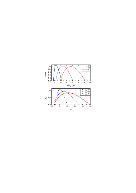
Figure 2: Distribution of energy transmitted between the resistors during time $t$ for different transmission probabilities $\tau(\omega)$. (a) $\tau(\omega)=$const, $T_{1}=300$ mK, $T_{2}=100$ mK, the observation time is $t=10$ ns. (b) $\tau(\omega)$ has the Lorentzian shape, $T_{1}=300$ mK, $T_{2}=100$ mK, $t=1$ ms, CGF is given by Eq. (39). Discrete number of transferred photons $n$ is shown on the horizontal axis.

III Results and discussion

Let us now consider some limiting cases. First we assume that the transmission probability, $\tau$, is constant and the photon distribution functions have equilibrium Bose form. In this case the heat current acquires familiar form $J_{Q}=-(i/t)dF/d\lambda|_{\lambda=0}=\pi\tau\left(T_{1}^{2}-T_{2}^{2}\right)/12.$ The simplest example of such a system is given by two directly connected resistors (Fig. 1e), in which case $\tau=4R_{1}R_{2}/(R_{1}+R_{2})^{2}$. In Fig. 2a we show the distribution $P(t,Q)$ for three different values of $\tau$. The distribution becomes Gaussian at sufficiently long observation time such that $J_{Q}t\gg T_{1}$. The low frequency noise of the heat current is given by the expression

$$S_{Q}=-\frac{1}{t}\frac{d^{2}F}{d\lambda^{2}}\bigg{|}_{\lambda=0}=\left(\frac{\zeta(3)}{\pi}\tau(1-\tau)+\frac{\pi}{6}\tau^{2}\right)(T_{1}^{3}+T_{2}^{3})$$

$$+\,2\tau(1-\tau)\int_{0}^{\infty}\frac{d\omega}{2\pi}\frac{\omega^{2}}{\left(e^{\omega/T_{1}}-1\right)\left(e^{\omega/T_{2}}-1\right)}.$$ (38)

Another interesting limit is transmission within a narrow Lorentzian with $\tau(\omega)=\tau_{\max}\Gamma^{2}/[(\omega-\omega_{0})^{2}+\Gamma^{2}]$ and $\Gamma\ll\omega_{0},T_{1},T_{2}$. In this case

$$F=-\Gamma t\left(\sqrt{1-\tau_{\max}f(\omega_{0})}-1\right),$$ (39)

where $f(\omega_{0})=n_{1}(\omega_{0})[1+n_{2}(\omega_{0})]\left(e^{i\lambda\omega_{0}}-1\right)+[1+n_{1}(\omega_{0})]n_{2}(\omega_{0})\left(e^{-i\lambda\omega_{0}}-1\right).$ Since $F(\lambda)$ becomes a periodic function of $\lambda$ in this approximation, we get $P(t,Q)=\sum_{n}p_{n}\delta(Q-n\omega_{0})$ with $p_{n}=\frac{\omega_{0}}{2\pi}\int_{-\pi/\omega_{0}}^{\pi/\omega_{0}}d\lambda\,e^{in\lambda\omega_{0}}e^{F(\lambda)}$ being the probability to transmit $n$ photons with one frequency $\omega_{0}$. The distributions $p_{n}$ for three different values of $\tau_{\max}$ are shown in Fig. 2b. Due to the suppression of the average heat current between the resistors the distributions $p_{n}$ significantly deviate from the Gaussian form even though the observation time is long, $t=1$ ms. It is obvious from Eq. (39) that the distribution $p_{n}$ becomes Poissonian in the limit $T_{1}\gg T_{2}$ and $\tau_{\max}\ll 1$. At higher transparencies it deviates from the Poissonian form similarly to what has been predicted in Ref. Schomerus, , where the statistics of photons emitted by a coherent conductor has been studied and rectangular shape of the transmission line has been assumed. The average heat current and the noise corresponding to CGF (39) are (here $n_{j}\equiv n_{j}(\omega_{0})$)

$$J_{Q}=\frac{\tau_{\max}}{2}\Gamma\omega_{0}[n_{1}-n_{2}],\;\;S_{Q}=\frac{\tau_{\max}}{2}\Gamma\omega_{0}^{2}\big{(}n_{1}[1+n_{2}]$$

$$+\,[1+n_{1}]n_{2}+\tau_{\max}[n_{1}-n_{2}]^{2}/2\big{)}.$$ (40)

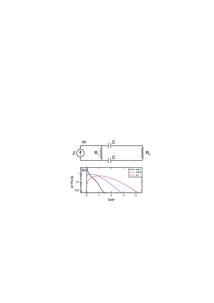
Figure 3: (a) Bias current $I$ is applied to the resistor 1 in order to drive it out of equilibrium. Two capacitors $C$, which shield the detector resistor 2 at low frequencies, are big enough to become fully transparent at frequencies $\omega\sim\max\{T_{1},T_{2},eV\}$, where $V=IR_{1}$. In this case the barrier transmission $\tau$ may be approximately treated as frequency independent constant. (b) Distribution of transmitted energy during the observation time $t=100/eV$ for three different values of $\tau$. $Q$ and $P(Q)$ are scaled with the characteristic photon energy $eV$.

Next we assume that leads are attached to the resistor 1 and bias current $I$ is applied to it (see Fig. 3a). The electron distribution function inside it acquires a non-equilibrium double step form Nagaev , $f(E,x)=(x/L_{1})f(E-eV)+(1-x/L_{1})f(E)$, where $V=IR_{1}$ is the voltage drop. We also assume that the temperatures of the resistor 2 and of the outer leads are much lower than $eV$. In this case one can put $n_{2}(\omega)=0$ and from the Eq. (25) we find $n_{1}(\omega)=(eV-\omega)\theta(eV-\omega)/6\omega$. Thus the CGF (36) takes the form

$$F=-t\int_{0}^{eV}\frac{d\omega}{2\pi}\ln\left[1-\frac{\tau}{6}\frac{eV-\omega}{\omega}\left(e^{i\lambda\omega}-1\right)\right].$$ (41)

The corresponding distribution $P(Q)$ is shown in Fig. 3b. It is strongly asymmetric with $P(Q)=0$ for $Q<0$, i.e. over long intervals of time, $eVt\gtrsim 1$, the energy flows from the biased resistor to the unbiased one, but never in the opposite direction. A somewhat similar system, namely a biased resistor coupled to an open transmission line, has been earlier considered in Ref. Ojanen, , where the average value of the heat current and its noise have been derived. From CGF (41) we find these parameters in our model

$$J_{Q}=\frac{\tau(eV)^{2}}{24\pi},\;\;S_{Q}=\left(1+\frac{\tau}{3}\right)\frac{\tau(eV)^{3}}{72\pi}.$$ (42)

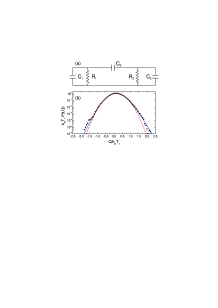
Figure 4: (a) Setup of the experiment Ciliberto1 ; Ciliberto2 . The circuit parameters are: $R_{1}=R_{2}=10$ M$\Omega$, $C_{0}=100$ pF, $C_{1}=680$ pF, $C_{2}=420$ pF. The parameters defined in the text take the values $\alpha=2.134$, $\beta=0.0506$, and $t_{0}=6.29$ ms. (b) Distribution of energy transmitted during the time $t=0.1$ sec and for resistor temperatures $T_{1}=296$ K, $T_{2}=88$ K. Circles – experimental pointsCiliberto1 ; Ciliberto2 ; blue line – Eq. (46); red dashed line – Gaussian approximation $P(t,Q)=\exp[-(Q-J_{Q}t)^{2}/2S_{Q}t]/\sqrt{2\pi S_{Q}t}$, where $J_{Q}$ and $S_{Q}$ are defined by Eqs. (47).

In the classical limit $T_{j}\gg\omega_{c}$ CGF (36) reduces to Saito2

$$F=-t\int_{0}^{\infty}\frac{d\omega}{2\pi}\ln\left[1-\tau(\omega)\left(i\lambda\Delta T_{12}-\lambda^{2}T_{1}T_{2}\right)\right],$$ (43)

where $\Delta T_{12}=T_{1}-T_{2}$. It is interesting to compare this result with the experimentCiliberto1 ; Ciliberto2 . In that experiment capacitors have been used, which implies $Z_{j}(\omega)=1/(-i\omega C_{j})$ (see Fig. 4a). Accordingly, $\tau(\omega)$ (37) takes the form

$$\tau(\omega)=\frac{2\beta(\omega t_{0})^{2}}{1+2(\alpha-1)(\omega t_{0})^{2}+(\omega t_{0})^{4}},$$ (44)

with $t_{0}=\sqrt{R_{1}R_{2}(C_{1}C_{2}+C_{0}C_{1}+C_{0}C_{2})}$,

$$\alpha=1+[R_{1}^{2}(C_{0}+C_{1})^{2}+R_{2}^{2}(C_{0}+C_{2})^{2}+2R_{1}R_{2}C_{0}^{2}]/2t_{0}^{2},$$

and $\beta={2C_{0}^{2}}/(C_{1}C_{2}+C_{0}C_{1}+C_{0}C_{2})$. For this model one can exactly evaluate CGF (43),

$$F=\frac{t}{t_{0}}\left(\sqrt{\frac{\alpha}{2}}-\sqrt{\frac{\alpha}{2}-\frac{\beta(i\lambda\Delta T_{12}-\lambda^{2}T_{1}T_{2})}{2}}\right),$$ (45)

and the distribution of the transferred heat $P(t,Q)=\int\frac{d\lambda}{2\pi}e^{-i\lambda Q+F(t,\lambda)}$, which reads

$$P(t,Q) = \frac{t}{\pi}\sqrt{\frac{2a}{\beta T_{1}T_{2}t^{2}+2Q^{2}t_{0}^{2}}}\,e^{\frac{t}{t_{0}}\sqrt{\frac{\alpha}{2}}+\frac{T_{1}-T_{2}}{2T_{1}T_{2}}Q}$$ (46)

$$K_{1}\left(\sqrt{a\left(\frac{t^{2}}{t_{0}^{2}}+\frac{2Q^{2}}{\beta T_{1}T_{2}}\right)}\right).$$

Here $K_{1}(x)$ is the modified Bessel function of the second kind, and $a=\alpha/2+\beta(T_{1}-T_{2})^{2}/8T_{1}T_{2}.$ One should bear in mind that the expression (46) is valid in the long time limit $t\gtrsim t_{0}$. The average heat current from the resistor 1 to the resistor 2 and the corresponding noise in this model have the form

$$J_{Q}=\frac{\beta(T_{1}-T_{2})}{2\sqrt{2\alpha}t_{0}},\;\;S_{Q}=\frac{\beta T_{1}T_{2}}{\sqrt{2\alpha}\,t_{0}}+\frac{\beta^{2}(T_{1}-T_{2})^{2}}{4\sqrt{2}\alpha^{3/2}t_{0}}.$$ (47)

We compare the distribution (46) with the experimental one Ciliberto1 ; Ciliberto2 in Fig. 4b. The agreement between the two is quite good. In particular, one can see the deviations from Gaussian form at the tails of the distribution. The subtle point of the measurements Ciliberto1 ; Ciliberto2 was the difference between the heat $Q_{1}$, i.e. the change of the energy of the resistor 1, and the work $W_{1}$, which also includes the change of the electrostatic energy of the capacitor $C_{1}$. We have verified that in the long time limit both $Q_{1}$ and $W_{1}$ should have the same distribution (46). On the qualitative level this can be understood from the relation $W_{1}=Q_{1}+C_{1}[V_{1}^{2}(t)-V_{1}^{2}(0)]/2$. Indeed, the average value of the last term, i.e. of the change in the energy of the capacitor $C_{1}$ during the observation time $t$, equals to zero because $\langle V_{1}^{2}(t)\rangle$ is finite and does not grow in time. Since both $Q_{1}$ and $W_{1}$ grow in time linearly, one can put $W_{1}\approx Q_{1}$ at sufficiently long $t$ even without averaging. Experimentally, however, the work distribution has approached the long time limit form faster than the heat distribution. That is why in Fig. 4b we plot the experimental work distribution $P(W_{1})$. Further analysis is required in order to understand the origin of this behavior.

We propose the distribution of heat in the low temperature quantum regime to be measured in the setup similar to the one used in the experiments [Meshke, ,Timofeev, ]. Namely, one would monitor the temperature of the detector resistor 2 in real time with the time resolution of the order of $t_{0}\approx 12\hbar/\pi\tau k_{B}T_{1}$, that is the time interval during which an average energy $k_{B}T_{1}$ is transferred from the resistor 1 to the resistor 2. Assuming $T_{1}=100$ mK and $\tau=3\times 10^{-4}$ one finds $t_{0}\approx 1$ $\mu$s, which is within the reach of current technologySimone . The expected magnitude of temperature fluctuations in the second resistor caused by fluctuations of heat flow may be estimated as $\delta T_{2}^{2}\approx 3\tau T_{2}t/\pi^{3}\hbar k_{B}\nu^{2}\Omega_{2}^{2}$, where $t$ is the observation time. For a resistor with the volume $\Omega_{2}=0.001$ $\mu$m³ made of copper (density of states $\nu\approx 10^{29}$ J^-1 $\mu$m^-3) and for $T_{2}=50$ mK and $t=100t_{0}$ one finds $\delta T_{2}\sim 15$ mK, which is measurable with currently available thermometers based on normal metal – superconductor tunnel junctionsSimone ; Klara . One can further optimize the system by, for example, designing the coupling circuit with narrow line transmission spectrum, or by using other types of temperature sensors like, e.g., recently proposed sensor based on an SNS Josephson junction Tero ; Jonas .

In summary, we have developed a theory of full counting statistics of heat exchange between two metallic resistors, which is valid both at high and at low temperatures, where the classical formula for the noise (1) can no longer be used. Fluctuations of the heat current in this system can be interpreted as scattering of photons by an effective potential barrier. In high temperature limit our results are in good agreement with recent experimentCiliberto1 ; Ciliberto2 . We acknowledge very useful discussions with S. Ciliberto, G. Lesovik, O. Saira and Y. Utsumi. We are grateful to S. Ciliberto for providing us with the experimental data. This work has been supported in part by the Academy of Finland (projects no. 272218 and 284594), and the European Union Seventh Framework Programme INFERNOS (FP7/2007- 2013) under grant agreement no. 308850.