Parallel optimized sampling for stochastic equations

Abstract

Stochastic equations play an important role in computational science, due to their ability to treat a wide variety of complex statistical problems. However, current algorithms are strongly limited by their sampling variance, which scales proportionate to $1/N_{S}$ for $N_{S}$ samples. In this paper, we obtain a new class of variance reduction methods for treating stochastic equations, called parallel optimized sampling. The objective of parallel optimized sampling is to reduce the sampling variance in the observables of an ensemble of stochastic trajectories. This is achieved through calculating a finite set of observables — typically statistical moments — in parallel, and minimizing the errors compared to known values. The algorithm is both numerically efficient and unbiased. Importantly, it does not increase the errors in higher order moments, and generally reduces such errors as well. The same procedure is applied both to initial ensembles and to changes in a finite time-step. Results of these methods show that errors in initially optimized moments can be reduced to the machine precision level, typically around $10^{-16}$ in current hardware. For nonlinear stochastic equations, sampled moment errors during time-evolution are larger than this, due to error propagation effects. Even so, we provide evidence for error reductions of up to two orders of magnitude in a nonlinear equation example, for low order moments, which is a large practical benefit. The sampling variance typically scales as $1/N_{S}$, but with the advantage of a very much smaller prefactor than for standard, non-optimized methods.

1 Introduction

Stochastic differential equations (SDEs) play a universal and important role in many disciplines requiring quantitative modeling [1, 2, 3, 4, 5, 6, 7, 8, 9]. Their practical advantage is that, when used to solve large statistical problems, the ability to randomly sample greatly reduces the complexity of treating the full distribution function. They are employed for treating problems ranging from statistical physics, chemistry and engineering through to economics, biology and financial modeling. As a result of this large field of applications, there is substantial literature on the algorithms used to solve them [10, 11, 12, 13, 14, 15], and these are generally different to methods for ordinary differential equations (ODEs).

This utility is not without a price. Such numerical algorithms typically utilize many independent trajectories. Any statistical result will therefore have a sampling variance that scales $1/N_{S}$ for $N_{S}$ random samples. This causes to a typical error $\epsilon_{S}$ that scales as $1/\sqrt{N_{S}}$, giving an error that only decreases slowly with the total computation time. Numerical algorithms generally aim to reduce the truncation error $\epsilon_{T}$ due to the discretization in time, giving an error of order $\left(\Delta t\right)^{-p}$ for methods of order $p$. Yet reducing the truncation error cannot reduce the total error to less than the sampling error. Since the sampling error is often a large part of the total error one has to deal with, reducing the truncation error has a limited effectiveness.

Here we propose a new class of reduced variance SDE algorithms called parallel optimized sampling or POS algorithms for short. This approach can provide extremely useful variance reduction compared to independent random sampling methods. The method locally eliminates sampling errors over a finite set of moments, up to numerical precision. Higher order moment errors are reduced also. Global sampling error improvement over a finite time interval is not as large as this, due to error propagation effects, but is still very substantial. Other variance reduction techniques that can also improve sampling errors include the use of low discrepancy (or quasi-random) sequences [16], and an extrapolated hierarchy of simulations [17], which we do not treat here.

To achieve our results, we introduce a modification of the standard independent stochastic trajectory approach. A set of $N_{S}$ trajectories is solved in parallel using an optimized algorithm. This gives an improvement that depends on the order of the statistical moment being calculated. The present method is a highly practical one, since the run time is still only linear in $N_{S}$. This means that the error reductions are of real value. If the run time scaled as $N_{S}^{2}$, and errors were reduced to $1/N_{S}$, the reductions would not be so useful, since the total computational overhead at fixed error would not change.

There is a close relationship between the present approach and methods of moment hierarchies [5] or cumulant expansions. These existing cumulant based methods have a major drawback. One must close the infinite hierarchy with an arbitrary ansatz at some finite order. If this is incorrect, the method will fail [18], and several examples exist for this problem. In fact, such cumulant hierarchies cannot in general be truncated consistently [19]. By contrast, our method requires no ansatz; it gracefully reduces in a consistent way to the usual, unbiased stochastic method at large sample sizes. It is a unification of moment hierarchy and stochastic methods.

We focus mostly on simple one-dimensional cases here for simplicity, except for one higher-dimensional example to illustrate the approach. Extensions of the POS method to cases of higher-order convergence in time will be treated elsewhere. However, as one example of potential applications, sampling errors can play a major role in quantum simulations using phase-space representations. The difficulty is that distribution tails may only be weakly bounded [20]. In such cases, sampling error can determine whether a quantum simulation is feasible or not. One approach to solving this problem is using weighted trajectory methods [21]. Another method, which was successfully used in treating long-range order in the fermionic Hubble model, is to impose global conservation laws [22]. The present approach has a more general applicability than either of these, but can also be combined with such earlier techniques.

The organization of the paper is as follows. In Section 2, we analyze the stochastic errors that can arise in computational methods for stochastic differential equations. In Section 3 sampling errors are reduced in initial observables by introducing a new type of stochastic noise generator. Numerical examples of this are treated in Section 4, showing that variance in selected moments can be reduced to machine precision. Next, in Section 5, this approach is extended to dynamical optimization of stochastic equation algorithms, with numerical examples given in the remaining sections. In Section 6 we start by treating single-step optimization, which ignores error-propagation. In Section 7, we demonstrate the global, or multi-step performance of these methods for a number of one-dimensional linear and nonlinear cases, showing that global sampling error variance is substantially reduced compared to traditional independent trajectory approaches, typically by at least an order of magnitude. Finally, Section 8 treats a two-dimensional example which has very similar behaviour. Section 9 gives our summary and conclusions.

2 Stochastic integration error

Stochastic integration involves both truncation errors due to finite step-size, and errors due to finite samples. In this section we analyze the performance of independent SDE methods by considering the overall resources needed to solve the equations for some given error. To explain the background to our approach, we show that increasing the convergence order is a less effective way to reduce errors than one might expect, because of a trade-off between the resources needed to reduce both truncation and sampling errors. As large ensembles are required to reduce sampling errors, we find that higher-order methods for SDEs, while undoubtedly useful, are not as effective as in ODE integration.

In the rest of this paper, we show how to overcome this problem by using parallel algorithms that reduce sampling errors.

2.1 Distributions and observables

We start by establishing our notation. The observables of a probability distribution function $P\left(t,\mathbf{x}\right)$ are the fundamental objects of interest in stochastic calculations. These are probability-weighted integrals of functions $o_{m}\left(\mathbf{x}\right)$ over $\mathbf{x}$:

$$\left\langle o_{m}\right\rangle=\int\mathrm{d}\mathbf{x}o_{m}\left(\mathbf{x}\right)P\left(t,\mathbf{x}\right).$$ (1)

In general, $\mathrm{d}\mathbf{x}$ is a Euclidean measure over a $d$-dimensional real or complex space of variables $\mathbf{x}$. The numerical examples given here will focus mainly on moments of one-dimensional distributions with $o_{m}(x)=x^{m}$, giving a vector whose error should be minimized:

$$\mathbf{o}=\left\{o_{1},\ldots,o_{M}\right\}.$$ (2)

With sampling methods, the time-evolution is solved by generating a number $N_{S}$ of independent sample paths $\mathbf{x}^{(n)}(t)$. This procedure is equivalent to approximating the true distribution by the sampled distribution defined as

$$P_{S}\left(t,\mathbf{x}\right)=\frac{1}{N_{S}}\sum_{n=1}^{N_{S}}\delta\left(\mathbf{x}-\mathbf{x}^{(n)}\left(t\right)\right).$$ (3)

We note that the initial value problem consists of defining an initial static distribution $P\left(\mathbf{x}\right)$ at $t=t_{0}$, and then sampling it with initial points $\mathbf{x}^{(m)}\left(t_{0}\right)$. For dynamics, the sampled paths are defined at $N_{T}$ discrete times $t_{i}$, with a spacing $\Delta t$, such that exact ensemble average values are recovered in the double limit of infinite sample and zero step-size:

$$\left\langle o_{m}\left(t_{i}\right)\right\rangle=\lim_{\Delta t\rightarrow 0}\lim_{N_{S}\rightarrow\infty}\frac{1}{N_{S}}\sum_{n=1}^{N_{S}}o_{m}\left(\mathbf{x}^{(n)}\left(t_{i}\right)\right).$$ (4)

These paths are obtained by numerical algorithms which propagate $\mathbf{x}^{(n)}(t_{i})$ to $\mathbf{x}^{(n)}(t_{i+1})$, with a truncation error vanishing as $\Delta t\rightarrow 0$. If we call $N_{S}$ the sample number, the phase-space is made up of a set of distinct samples or trajectories. These form an extended vector of parallel trajectories,

$$\mathbf{X}=\left(\begin{array}[]{ccc}\mathbf{x}^{(1)T}&\cdots&\mathbf{x}^{(N_{S})T}\end{array}\right)^{T},$$ (5)

of size $N_{S}d$. It is convenient to define the sampled observables as a function $\bar{\mathbf{o}}$ of the extended vector of sampled trajectories,

$$\bar{o}_{m}\left(\mathbf{X}\right)=\frac{1}{N_{S}}\sum_{n=1}^{N_{S}}o_{m}\left(\mathbf{x}^{(n)}\right).$$ (6)

Throughout this paper, we will use the standard notation that all extended vectors or matrices involving a dimension of the order of the sample size $N_{S}$ are written in upper case like $\mathbf{X}$, while objects that do not depend on the sample size are written in lower case.

2.2 Fokker-Planck and stochastic equations

To explain the problem of interest here, we give a detailed analysis of a stochastic differential equation or SDE. The underlying distribution function $P\left(t,\mathbf{x}\right)$ satisfies the Fokker-Planck equation [6],

$$\frac{\partial P\left(t,\mathbf{x}\right)}{\partial t}=\left[-\sum_{i}\frac{\partial}{\partial x_{i}}a_{i}(\mathbf{x})+\frac{1}{2}\sum_{ij}\frac{\partial^{2}}{\partial x_{i}\partial x_{j}}\mathsf{d}_{ij}(\mathbf{x})\right]P\left(t,\mathbf{x}\right)\,.$$ (7)

We wish to minimize the errors for solving the corresponding Itō SDE [4, 6], given in a standard form by:

$$\mathrm{d}\mathbf{x}=\mathbf{a}\left(\mathbf{x}\right)\mathrm{d}t+\bm{\mathsf{b}}\left(\mathbf{x}\right)\mathrm{d}\mathbf{w},$$ (8)

where $\bm{\mathsf{d}}=\bm{\mathsf{b}}\bm{\mathsf{b}}^{T}$, and the Gaussian distributed real noise $\mathrm{d}\mathbf{w}$ has correlations given by:

$$\left\langle\mathrm{d}w_{i}\mathrm{d}w_{j}\right\rangle_{\infty} = \delta_{ij}\mathrm{d}t$$

$$\left\langle\mathrm{d}w_{i}\right\rangle_{\infty} = 0.$$ (9)

Here the $\left\langle\dots\right\rangle$ notation means ensemble average, so that

$$\left\langle\mathbf{x}\right\rangle_{N_{S}}\equiv\frac{1}{N_{S}}\sum_{n=1}^{N_{S}}x^{(n)},$$ (10)

with $\langle\dots\rangle_{\infty}$ being the infinite ensemble limit.

2.3 Sampling and error criteria

To evaluate the computational error, we must define an error criterion relevant to the entire sample ensemble $\mathbf{X}$. In practical terms, this means one must calculate errors in each required observable, rather than just the errors in a single trajectory. By minimizing the total error over a finite number of samples, one should be able to arrive at the most efficient algorithm that utilizes a given computational resource.

To quantify the error we will use a weighted norm $\left\|P\right\|_{W}=\sqrt{\left(P,P\right)}\geq 0$. The integration error of a sampled, calculated stochastic distribution $P_{S}$ relative to the exact distribution $P_{E}$ is then defined as

$$\epsilon=\left\|P_{S}-P_{E}\right\|_{W},$$ (11)

which depends on the choice of weighted norm.

The computed averages, $\left\langle o_{m}\right\rangle_{P_{S}}$, are obtained through sampling, which means that typically one is interested in calculating specific observables with minimum error. To evaluate the computational accuracy relevant to these observables of interest, we choose a particular set of observable quantities, $o_{m}$, for $m=1,\ldots M$, to define the distribution norm, so that:

$$\left\|P\right\|_{W}^{2}\equiv\sum_{m=1}^{M}W_{m}\left|\left\langle o_{m}\right\rangle_{P}\right|^{2}.$$ (12)

Here $W_{m}$ is the relative weight assigned to observable $m$. We assume the error is evaluated at a fixed time $t$, otherwise one may wish to minimize the errors at each of a set of sample times. In most of this paper, the observables are a finite set of one-dimensional moments, $o_{m}\equiv x^{m}$, although other measures are certainly possible. For simplicity, we choose $W_{m}=1$ from now on.

With this definition, the total error is

$$\epsilon=\sqrt{\sum_{m=1}^{M}\left|\left\langle o_{m}\right\rangle_{P_{S}}-\left\langle o_{m}\right\rangle_{P_{E}}\right|^{2}},$$ (13)

The integration error $\epsilon$ clearly must be calculated from the entire vector of stochastic trajectories $\mathbf{x}$. The task of defining an optimal stochastic integration method is to obtain $\mathbf{x}\left(t\right)$ with a procedure that minimizes the total error $\epsilon$ relative to some computational resource. Using the definition that

$$\mu_{m}=\left\langle o_{m}\right\rangle_{P_{E}},$$ (14)

we see that:

$$\epsilon=\sqrt{\sum_{m=1}^{M}\left|\bar{o}_{m}\left(\mathbf{X}\right)-\mu_{m}\right|^{2}}.$$ (15)

Although different to the usual probability norms, we will use the above definition throughout this paper, since it corresponds to the operational requirements of a norm for a sampled distribution. For a single observable, say $x$, $\epsilon^{2}$ is simply the usual sample variance in $x$ — provided there are no other errors present as well. However, there are usually other errors, including errors due to arithmetic roundoff and the finite step-size of the integration algorithm.

2.4 Optimizing the sample number

What is the optimal strategy to solve this SDE, given fixed total computational resources and a goal of minimizing the total error? With independent paths, the computational resource utilized is proportional to $N=N_{S}N_{T}$, where $N_{S}$ is the number of samples and $N_{T}$ is the number of time-steps. One can invest total processing time either in reducing the time-step, or in increasing the number of samples, but reducing the step-size means using less samples, and vice-versa.

To understand these issues quantitatively, we first consider the optimal strategy for error-reduction with traditional methods that involve using independent sample paths. We will show that it is only important to reduce the step-size or discretization error to the point where it is some fraction of the sampling error.

Consider the total error for $N_{T}$ time-steps with a stochastic integration method of global order $p$, that utilizes $N_{S}$ independent sample paths. From the central limit theorem, the global sampling error $\epsilon_{S}$ due to the use of a finite sample, is

$$\epsilon_{S}=\sigma N_{S}^{-1/2},$$ (16)

where $\sigma$ is the standard deviation of the measured quantity, and the same type of scaling holds for sums over errors in multiple observables.

There are additional errors $\epsilon_{T}$ over a fixed time interval $T=N_{T}\Delta t$, due to the finite time-step $\mathrm{\Delta}t$. If the local error of one time-step is $\epsilon_{\mathrm{\Delta}t}$, then at best $\epsilon_{T}\approx N_{T}\epsilon_{\mathrm{\Delta}t}$. The discretization order $p$ is therefore defined so that the global time-step truncation error $\epsilon_{T}$ scales as

$$\epsilon_{T}=cN_{T}^{-p}\propto\Delta t^{p},$$ (17)

where $c$ is an algorithm-dependent constant that depends on the set of computed observables.

Since the two error sources are independent, the overall error is given approximately by a sum of two terms:

$$\epsilon=\epsilon_{T}+\epsilon_{S}=cN_{T}{}^{-p}+\sigma N_{S}^{-1/2}.$$ (18)

We wish to constrain the total processor time — parallel or otherwise — so that $N_{S}N_{T}=N$ is bounded. The total CPU time is then $T_{\mathrm{CPU}}=N\tau$, if one step in time takes a real time duration $\tau$, and other overheads are negligible.

Next, consider how to optimize the tradeoff between the truncation and sampling errors. Letting $\tilde{c}=cN^{-p}$, and keeping $N$ fixed, one obtains:

$$\epsilon=\tilde{c}N_{S}^{p}+\sigma N_{S}^{-1/2}$$ (19)

This is minimized by choosing a combination of time-step and sample number such that:

$$N_{S} = N^{\frac{2p}{2p+1}}\left[\frac{\sigma}{2pc}\right]^{\frac{2}{2p+1}}$$

$$N_{T} = N^{\frac{1}{2p+1}}\left[\frac{\sigma}{2pc}\right]^{-\frac{2}{2p+1}}$$ (20)

The total error is then:

$$\epsilon=\left[\frac{c\sigma^{2p}}{2pN^{p}}\right]^{\frac{1}{2p+1}}\left[1+\frac{1}{2p}\right]$$ (21)

2.5 Effective integration order

From the analysis above, the best that one can do to reduce errors is to obtain a scaling of $\epsilon\propto N^{-p_{\mathrm{eff}}}$, where the effective order $p_{\mathrm{eff}}$ is

$$p_{\mathrm{eff}}=\frac{p}{2p+1}.$$ (22)

This is because a higher order integration technique has no effect on the sampling error, which eventually dominates the error calculation. The best effective order, even with $p=\infty$, is $p_{\mathrm{eff}}=1/2$. Given that stochastic higher order algorithms are complex and slow, higher $p$ values are not always an advantage.

This optimal effective order requires the use of an optimal ratio of samples to steps, which is:

$$\frac{N_{S}}{N_{T}}=N^{\frac{2p-1}{2p+1}}\left[\frac{\sigma}{2pc}\right]^{\frac{4}{2p+1}}\,.$$ (23)

This ratio is difficult to calculate a-priori, since these constants are not usually known in advance. One can estimate the sampling error numerically by measuring the sample standard deviation $\sigma$, which is known from the statistics of the simulation. The truncation error constant $c$ is also measurable by changing the step-size. Thus, both $c$ and $\sigma$ can be measured in software. An optimum point is reached when the ratio between discretization and sampling error is given by the extremely simple result that:

$$\frac{\epsilon_{T}}{\epsilon_{S}}=\frac{1}{2p}\,.$$ (24)

In summary, it is only productive to reduce the step-size to the point where the discretization error of $1/2p$ of the sampling error. After this point is reached, one is better off to use more samples. Another way to describe this is that the least computational cost for error $\epsilon$ is

$$N\propto\epsilon^{-1/p_{\mathrm{eff}}}=\epsilon^{-\left(2p+1\right)/p}.$$ (25)

There are multi-scale methods [17] that can achieve a cost of $N\propto\epsilon^{-2}\left(\log\epsilon\right)^{2}$, which is a useful further improvement.

In summary, from the traditional analyses of ODE integration, one might expect that the error would be reduced extremely rapidly with a higher order method. This is not the case with an SDE. Because the independent sampling error varies slowly with resource, this becomes the dominant error with increasing resources.

Our conclusion is that sampling error strongly limits the effectiveness of independent sampling methods for SDEs.

3 Initial conditions for parallel optimized sampling

We now describe a family of variance reduction methods using parallel optimized sampling (POS), which locally eliminate sampling errors for a finite set of observables $\mathbf{o}$, thus improving computational efficiency. As described above, for $N_{S}$ samples, there is a $N_{S}d$-dimensional extended vector of stochastic variables, $\mathbf{X}=\left(\begin{array}[]{ccc}\mathbf{x}^{\left(1\right)T}&\cdots&\mathbf{x}^{\left(N_{S}\right)T}\end{array}\right)^{T}$, which is optimized so that $\mathbf{X}\rightarrow\mathbf{X}^{(\mathrm{opt})}$ . Both initial samples and the resulting stochastic trajectories are optimized in parallel, thus making use of increasingly parallel hardware capabilities.

Before deriving the POS algorithm, we need to address an issue arising from the known initial condition for the SDE, with $\mathbf{x}$ having a distribution $P\left(\mathbf{x}\right)$ at $t=t_{0}$. When we derive the optimization conditions, one of the assumptions will be that the moments of $\mathbf{x}$ are already optimized at the start of each time step, that is $\langle o_{m}\left(t\right)\rangle_{N_{S}}=\mu_{m}\left(t\right)$ for $m=1\dots M$. At every step of the SDE integration, if we obtain the optimized stochastic vector from the previous step, then, since we optimize the differentials of the moments, the resulting stochastic variables will be optimized as well as possible, apart from any time-step errors, which is a separate issue.

But how do we ensure the initial set of moments of the distribution $P\left(\mathbf{x}\right)$ is optimized at the first integration step?

3.1 Static POS

We emphasize that our main goal is to minimize the variance for the dynamical stochastic equations, treated next. As a consequence, we do not use methods like Gaussian quadratures for the static variance reduction problem. These are limited in the diversity of initial distributions treated, and they cannot be easily generalized to the dynamic case. Instead we take a set of random samples from $P\left(\mathbf{x}\right)$, and optimize these initial sampled variables to reduce the variance in moments of interest.

We call this static POS, as it does not involve dynamical time-evolution. In other words, we wish to sample the initial values for the trajectories so that $M$ chosen observables are equal to their known exact values, that is,

$$\bar{\mathbf{o}}\left(\mathbf{X}\right)=\bm{\mu}\equiv\langle\mathbf{o}\rangle_{\infty},$$ (26)

where $\boldsymbol{\mu}$ is an $M$-dimensional vector. That is, we wish to set $\epsilon_{P}=\epsilon_{P}(t_{0})=0$, where $\epsilon_{P}$ is the total error (15) in the initial distribution, using an observable-based error measure. In the examples given in this paper, we treat all moments up to a given order. More generally, at high dimension $d$, treating all correlations or moments to a fixed order is exponentially hard. Therefore, it is necessary to select moments according some importance criterion, the effects of which will be treated in a later publication.

This is a classic example of nonlinear, multidimensional root-finding, with optimization over the dimensionality of the full space of samples. It can be a challenge to solve these equations efficiently, with resources no greater than $\mathcal{O}(N_{S})$, and with minimal changes to the original sampled estimate for $\mathbf{X}(t_{0})$, which is labelled $\mathbf{X}_{(0)}$. However, in examples treated here, we find that the numerical problem can be very accurately solved, naturally with machine-limited numerical precision. Here we use an iterative, modified Newton-Raphson method for the solution. Other techniques are available as well.

In an iterative Newton-Raphson approach, we use stochastic methods for the first estimate, $\mathbf{X}_{(0)}$. At each iteration, we set $\mathbf{X}\rightarrow\mathbf{X}+\delta\mathbf{X}$ to obtain the next estimate $\mathbf{X}_{(i+1)}$, which has a better fit to the required moments, so that $\mathbf{X}_{(i+1)}=\mathbf{X}_{(i)}+\delta\mathbf{X}_{(i+1)}$, where $\|\delta\mathbf{X}_{(i+1)}\|\ll\|\boldsymbol{X}_{(i)}\|$, and $\|\dots\|$ denotes the Euclidean norm.

Expanding to first order in $\delta\mathbf{X}_{(i+1)}$, the conditions we require are:

$$\bar{\mathbf{o}}^{\mathrm{(opt)}} = \bm{\mu}$$ (27)

$$= \bar{\mathbf{o}}\left(\mathbf{X}_{(i)}\right)+\bm{\mathsf{J}}\left(\mathbf{X}_{(i)}\right)\delta\mathbf{X}_{(i+1)}+\mathcal{O}\left(\delta\mathbf{X}_{(i+1)}^{2}\right),$$

where $\bm{\mathsf{J}}$ is a Jacobian of $\bar{\mathbf{o}}$:

$$\mathsf{J}_{mn}\left(\mathbf{X}\right)=\frac{\partial\bar{o}_{m}\left(\mathbf{X}\right)}{\partial X_{n}}\,.$$ (28)

In matrix form, the iteration equation is therefore

$$\bm{\mathsf{J}}_{(i)}\delta\mathbf{X}_{(i+1)}=\bm{\mu}-\bar{\mathbf{o}}_{(i)}.$$ (29)

where we use the obvious notation that $\bar{\mathbf{o}}_{(i)}\equiv\bar{\mathbf{o}}\left(\mathbf{X}_{(i)}\right)$ and $\bm{\mathsf{J}}_{(i)}\equiv\bm{\mathsf{J}}\left(\mathbf{X}_{(i)}\right)$. We note that out method is scale-invariant in the sense that it will result in the exact same solutions if we rescale any observable and its exact value as $o_{i}(\mathbf{X})\rightarrow c_{i}o_{i}(\mathbf{X})$, where $c_{i}$ is a constant.

Each step of the iterative solution is underdetermined, since the relevant matrices are not square, and hence not invertible. Such problems are relatively common in optimization, and here we analyze two different techniques to solve them.

3.2 One-dimensional example of iteration equations

We will use as an illustrative example the situation when the observables are moments of a one-dimensional stochastic equation. In this example $o_{m}=x^{m}$, so the conditions are:

$$\left[\mathbf{X}^{\mathrm{(opt)}}\right]^{m}\cdot\mathbf{1} = N_{S}\mu_{m}$$ (30)

$$= \mathbf{X}_{(i)}^{m}\cdot\mathbf{1}+m\mathbf{X}_{(i)}^{m-1}\cdot\delta\mathbf{X}_{(i+1)}+\mathcal{O}\left(\delta\mathbf{X}_{(i+1)}^{2}\right),$$

where the powers of matrices and vectors are understood in the element-wise (Hadamard) sense (e.g., $\mathbf{X}^{2}\equiv\mathbf{X}\circ\mathbf{X}$). Hence, in this case the observable vector and matrix of derivatives are:

$$\bar{\mathbf{o}}\left(\mathbf{X}\right) = \frac{1}{N_{S}}\sum_{n=1}^{N_{S}}\left(\begin{array}[]{c}x^{(n)}\\ \cdots\\ {}[x^{(n)}]^{M}\end{array}\right),$$ (34)

$$\bm{\mathsf{J}}\left(\mathbf{X}\right) = \frac{1}{N_{S}}\left(\begin{array}[]{ccc}1&\cdots&1\\ &\cdots\\ M\left[x^{(1)}\right]^{M-1}&\cdots&M\left[x^{(N_{S})}\right]^{M-1}\end{array}\right).$$ (38)

3.3 Static iteration solution with a matrix pseudo-inverse

The simplest method to solve the iteration equation (29) is to use a matrix pseudo-inverse. This has another advantage, since the pseudo-inverse has the property that it generates a least-squares solution, with minimal changes, as required for this algorithm.

Thus, we have the iterative procedure

$$\mathbf{X}_{(i+1)}=\mathbf{X}_{(i)}+\bm{\mathsf{J}}_{(i)}^{+}\left(\bm{\mu}-\bar{\mathbf{o}}_{(i)}\right).$$ (39)

where $\bm{\mathsf{J}}^{+}$ indicates the pseudo-inverse of the $M\times N_{S}$ Jacobian $\bm{\mathsf{J}}$.

This pseudo-inverse method is simple, general and effective. It satisfies our requirements given above. However, standard pseudo-inverse software using singular value decomposition (SVD) methods has drawbacks. It is relatively slow, can have stability problems and may not be available on all programming platforms.

3.4 Improved matrix inversion iterations

To improve efficiency and overcome problems with the use of general purpose pseudo-inverses, there is a faster alternative method for solving (29).

The pseudo-inverse is a limit. If $\bm{\mathsf{J}}^{\dagger}$ denotes the conjugate transpose of the matrix $\bm{\mathsf{J}}$, then:

$$\bm{\mathsf{J}}^{+}\equiv\lim_{\alpha\rightarrow 0}\bm{\mathsf{J}}^{\dagger}\left(\bm{\mathsf{J}}\bm{\mathsf{J}}^{\dagger}+\alpha\mathbf{I}\right)^{-1}.$$ (40)

Hence, provided $\bm{\mathsf{u}}=\bm{\mathsf{J}}\bm{\mathsf{J}}{}^{\dagger}$ is invertible, one can directly obtain that $\bm{\mathsf{J}}^{+}=\bm{\mathsf{J}}^{\dagger}\bm{\mathsf{u}}^{-1}$. It is important to note here that $\bm{\mathsf{u}}$ is only an $M\times M$ matrix, regardless of how many samples were used originally.

This gives as many unknown coefficients as there are equations. As a result, we only need solve $M$ linear equations in $M$ unknowns, for which there are efficient techniques, resulting in the iteration procedure

$$\mathbf{X}_{(i+1)}=\mathbf{X}_{(i)}+\bm{\mathsf{J}}_{(i)}^{\dagger}\bm{\mathsf{u}}_{(i)}^{-1}\left(\bm{\mu}-\bar{\mathbf{o}}_{(i)}\right).$$ (41)

Here the matrix $\bm{\mathsf{u}}$ being inverted is an $M\times M$ positive-semidefinite matrix. We use the lower case for it to indicate that it does not take an extended dimensionality. It is generally invertible and relatively small compared to the sample size, resulting in a highly efficient optimization algorithm. Numerical investigations show that this simple method is convergent for large sample number $N_{S}$, which corresponds to cases where the initial sample has moments close to their ideal values.

As the stopping condition in the numerical examples given later, we choose the condition that the changes are small relative to the modulus of the current $\mathbf{X}$ value, i.e. $\|\delta\mathbf{X}_{(i+1)}\|/\|\mathbf{X}_{(i)}\|<\eta=10^{-8}$, where $\eta^{2}$ is the numerical machine precision, as previously. An iteration limit of $I_{\max}=50$ was used, although as we see later, the typical iteration number is much lower than this.

We note that this simplified method is only useful when $\bm{\mathsf{u}}$ is invertible, otherwise the full SVD techniques or other more robust algorithms should be used. This is not a major limitation: as long as the first derivatives of our observables are linearly independent, $\bm{\mathsf{u}}$ will be invertible. As often the case with such numerical methods, performance can be further improved through linear scaling or translation operations.

However, sometimes the Newton-Raphson method doesn’t converge, not because $\bm{\mathsf{u}}$ lacks invertibility (which is rare), but because the initial guess is too far away from the solution. This can be detected by checking if the norm of $\bm{\Delta}$ increases. In such cases, one can back-track and try again with a different initial estimate. In the case of time-evolution dynamics, treated next, a smaller time-step can also be used to ensure the initial guess is close to hte solution.

3.5 One-dimensional case: power series method

As an equivalent way to understand our approach in the one-dimensional case, we can expand $\delta\mathbf{X}$, which is the iterative change in $\mathbf{X}$, using the derivative matrix and a vector of changes in observables, $\delta\mathbf{o}$. With observables as moments, this is a series in $\mathbf{X}^{\dagger}$ up to order $M-1$, with $M$ coefficients written as a vector $\bm{\delta}$. The expansion is given by:

$$\delta\mathbf{X}=\bm{\mathsf{J}}^{\dagger}\delta\bar{\mathbf{o}}=\frac{1}{N_{S}}\sum_{m=1}^{M}m\left(\mathbf{X}^{\dagger}\right)^{m-1}\delta\bar{o}_{m}.$$ (42)

Defining a square, positive definite matrix:

$$\bm{\mathsf{u}}_{(i)}=\bm{\mathsf{J}}_{(i)}\bm{\mathsf{J}}_{(i)}^{\dagger},$$ (43)

the basic iteration equation (29) becomes:

$$\bm{\mathsf{u}}_{(i)}\delta\bar{\mathbf{o}}{}_{(i+1)}=\bm{\mu}-\bar{\mathbf{o}}_{(i)}.$$ (44)

Since the solution for $\bm{\delta}{}_{(i+1)}$ requires the inversion of $\bm{\mathsf{u}}_{(i)}$, this leads to the same final algorithm that is defined above, in Eq (41).

4 Numerical examples: Static optimization

In this section, we perform numerical optimizations of initial conditions, following the methods of the previous section. This is important because the initial sampling error can dominate the sampling error found throughout the calculation, if it is not optimized. For definiteness, in most of the numerical examples of POS algorithms analyzed here, the $m$-th observable is a finite moment of a one-dimensional real distribution. Hence,

$$\bar{o}_{m}\equiv\left\langle o_{m}\right\rangle_{N_{S}}=\frac{1}{N_{S}}\sum_{n=1}^{N_{S}}\left[x^{(n)}\right]^{m}=\frac{\mathbf{X}^{m}\cdot\mathbf{1}}{N_{S}},$$ (45)

where $\mathbf{1}$ is an $N_{S}$-dimensional unit column vector. We optimize moments, for $m=1,\dots M$. As well as calculating the resulting error in these optimized moments, we also obtain the errors in other moments. An important issue is that the non-optimized moments should not have increased errors. We will also consider the ensuing results for two less regular observables: $o_{\exp}(x)=\exp(x)$ (a combination of an infinite number of moments) and $o_{||}(x)=|x|$ (an irregular function).

4.1 Static optimization

In this section we will test the performance of the iterative algorithm from Section 3 applied to the most common initial condition — a normal distribution. However, we emphasize that this choice is purely for convenience, and any initial distribution could be used. In this section we will use $\mu=\mu_{1}=0$ for all the tests and set the variance $\sigma^{2}=\mu_{2}=1$. This helps to avoid precision loss when calculating central moments, which is important, since the method is extremely efficient and optimizes the moments almost to the limit of numerical precision, as seen below. If maximum precision is required for cases when $\mu\neq 0$, one can subtract the mean of the initial distribution so that $\mu=0$ in the new variables.

With $\mu=0$, the moments of the test distribution are given by

$$\mu_{m}=\left\{\begin{array}[]{cc}0,&m\ \mathrm{is\ odd},\\ \sigma^{m}\left(m-1\right)!!,&m\ \mathrm{is\ even}.\end{array}\right.$$ (46)

The number of moments being optimized here is $M=6$, but this is not essential. For the additional observables the expected values are the expectation of the log-normal distribution

$$\mu_{\exp}=\exp\left(\frac{\sigma^{2}}{2}\right),$$ (47)

and the expectation of the folded normal distribution

$$\mu_{||}=\sigma\sqrt{\frac{2}{\pi}}.$$ (48)

We test the behavior of the algorithms in $10000$ independent optimization attempts, each with $N_{S}=1000$ parallel samples, in order to collect statistics. In each attempt, a $N_{S}$-dimensional vector $\mathbf{X}$ is generated using random sampling and the matrix inversion iterative method from Section 3.4 is applied to it. We then plot the distribution of measures of interest, which indicate the performance of the method. This demonstrates how well the algorithm performs when tested over a range of different initial random samples, each drawn from the same underlying normal distribution.

4.2 Distribution of the optimized variance reduction

There are several quantities we are interested in. We first investigate the distribution of the optimized variance. This gives an idea of not just how much the variance is reduced, but also the probability of a given amount of variance reduction.

Figure 1: Distribution of normalized errors in the static optimization tests for the matrix inversion method with $\sigma=1$, $N_{S}=1000$ (solid blue lines). The grey dotted curves show the normalized errors of a randomly sampled vector. The dash-dotted line denotes the numerical precision limit ($\epsilon_{\mathrm{num}}\approx 2.22\times 10^{-16}$ for double precision floating point numbers). Zero error results are removed from binning for ease of plotting.

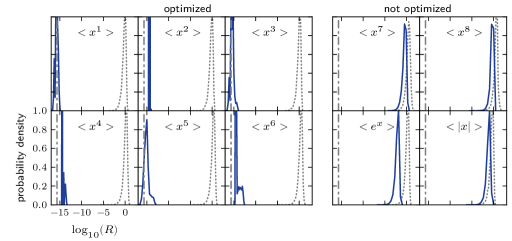
In more detail, we plot the numerically obtained distribution of final central moments of the vector compared to the desired values:

$$\tilde{R}_{m}\left(\mathbf{X}\right)=\left|\frac{1}{N_{S}}o(\mathbf{X})\cdot\mathbf{1}-\mu_{m}\right|,$$ (49)

where we will compare this quantity for initial randomly sampled vectors and optimized vectors. It is convenient to scale this to the expectation of the error in the sampled moment (for random samples) for the normal distribution:

$$R_{m}=\frac{\tilde{R}_{m}}{\sigma^{m}\sqrt{m!/N_{S}}},$$ (50)

so the average of $R_{m}$ for the initial randomly sampled vectors will be close to $1$ for all $m$. Fig. 1 shows this quantity both for the moments we are optimizing ($m=1\dots M$) and for two higher moments that are not optimized. The errors for the additional observables are normalized simply as

$$R_{\exp,||}=\frac{\tilde{R}_{\exp,||}}{\sqrt{N_{S}}}.$$ (51)

The optimization procedure was able to reduce errors almost to the limit of numerical precision of $R_{m}\sim 10^{-15}$ in many cases. The moments that were not directly optimized show some improvement as well, but typically closer to a single order of magnitude. Since we use logarithmic graphs, and $R_{m}$ can sometimes be zero, we excluded these zero results from the binning.

4.3 Number of iterations and optimization distance

It is also useful to know the number of iterations performed in each of the algorithms. This gives an idea of the numerical cost, which we investigate in greater detail below. If too many iterations are needed, the time taken will increase to the point that one may as well use more traditional methods.

Figure 2: (a) Number of iterations taken by the matrix inversion method, $\sigma=1$, $N_{S}=1000$. (b) Relative distance $D$ between the optimized vector and the initial randomly sampled vector in the static optimization tests for the matrix inversion method, $\sigma=1$, $N_{S}=1000$. (c) Average relative distance $\langle D\rangle$ depending on the number of trajectories $N_{S}$ in the static optimization tests for the matrix inversion method, $\sigma=1$. The grey dashed line denotes the slope of a $1/\sqrt{N_{S}}$ dependence.

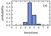
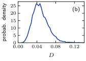
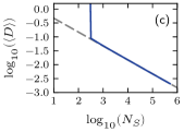
Fig. 2(a) demonstrates that only a small number of iterations — typically four — are necessary for the method to converge, given a reasonably large ensemble. The third quantity of interest is the relative distance of the optimized vector from the initial randomly sampled one:

$$D=\frac{\|\mathbf{X}^{(\mathrm{opt})}-\mathbf{X}\|}{\|\mathbf{X}\|}.$$ (52)

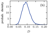
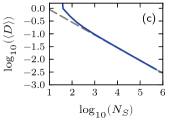
We would like this to be much less than $1$, which means that the optimized vector is still approximately “random”. Fig. 2(b) shows that it is indeed the case, and the average deviation is $D\approx 5\times 10^{-3}$ for $\sigma=1$. Fig. 2(c) shows that the results have the desirable property that the relative distance between the optimized and non-optimized trajectories scales with $1/\sqrt{N_{S}}$. This is expected from the fact that the initial sampled moment relative errors scale as $1/\sqrt{N_{S}}$, hence one expects the minimum required change to be of this order.

However, if there are too few trajectories, the simple matrix inversion iteration method diverges, producing unacceptably large changes $D$ in the distribution. For these small $N_{S}$ values, the iteration limit of $I_{\max}=50$ was reached, indicating a lack of convergence.

Figure 3: Dependence of normalized errors on the number of trajectories $N_{S}$ in the static optimization tests for the expansion method, $\sigma=1$. The dotted curve shows the dependence for randomly sampled vectors.

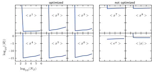
To investigate this more carefully, the dependence of the final error $R$ on the number of trajectories $N_{S}$, is plotted in Fig. 3. The results also display a sharp cut-off in the number of trajectories below which the iterative approach does not converge. More robust minimization algorithms could presumably solve this, but the issue was not investigated here for space reasons.

4.4 Initial optimization cost

For practical applications, the time taken for the optimization is also important. More accurately, the quantity of interest is the efficiency [23], which in our case can be expressed as $\mathrm{Eff=1/\left(T_{\mathrm{CPU}}\tilde{R}^{2}\right)}$, where $T_{\mathrm{CPU}}$ is the time required to generate the vector $\mathbf{X}^{(\mathrm{opt})}$.

Figure 4: Dependence of the cost on the number of trajectories $N_{S}$ in the static optimization tests for the expansion method, $\sigma=1$. The dotted curve shows the dependence for randomly sampled vectors.

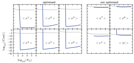
Since in our case in a significant fraction of optimization attempts $\tilde{R}$ for optimized moments is exactly zero, we plot the cost

$$\mathrm{Cost}=\frac{1}{\mathrm{Eff}}\equiv T_{\mathrm{CPU}}\tilde{R}^{2}.$$ (53)

averaged over attempts. Fig. 4 shows this quantity for all investigated observables. For the optimized moments ($m=1\dots 6$) the cost of POS is significantly lower than the cost of the purely random sampling (starting from a certain critical number of trajectories). The situation is different for non-optimized observables, where POS still demonstrates a decreased cost, but the difference is not as overwhelming.

In conclusion, the expansion iterative method performs well for a wide range of parameters, while being fast and easy to implement. Convergence is extremely rapid when the number of stochastic trajectories is increased above a critical value. However, we note that many other methods of nonlinear root-finding exist, and we do not exclude the possibility of better techniques being available.

We use this approach in the SDE examples given below, to pre-optimize the starting conditions for the SDE integration tests.

5 Parallel dynamic optimization

The general approach here is to assume that samples with an optimized set of observables are known at a given time $t$. Given this, a noise ensemble is chosen to give the lowest possible errors in the observables at a later time $t+\Delta t$. Overall convergence is then achieved by taking a large $N_{S}$ limit. The goal of the algorithm is that the observable moments are obtained with minimal error. For efficiency, the resulting calculation complexity should be linear in $N_{S}$.

In summary, the POS algorithm must therefore meet three essential requirements:

1. Equations for a finite set of $M$ observables are optimized both initially, and for local changes in time to a given order in $\Delta t$.

2. Non-optimized observables still have their correct values to the same order in $\Delta t$ in the limit of $N_{S}\rightarrow\infty$.

3. The computational cost of the algorithm should be no worse than $\mathcal{O}(N_{S})$.

If the observables chosen are moments, then, since higher order moments depend on lower order ones, these will experience a degree of optimization as well, even though not directly optimized. POS methods can also be combined with higher-order time-step methods, but here we focus on sampling error reduction for ease of explanation. Other types of observable also experience a degree of variance reduction as well. Typically this is not as great as experienced by the optimized moments, but this depends on the observable and the stochastic equation.

There is an analogy between this approach and the method of moment hierarchies in statistical physics [5]. The difference is that rather than an arbitrary truncation of the moment hierarchy, the higher order moments are estimated in an unbiased way via sampling.

We now describe how to extend this initial optimization algorithm to treat dynamical optimization of moments during stochastic time evolution of $\mathbf{x}$. This involves stochastic noise terms and deterministic drift terms.

5.1 Euler-Maruyama algorithm

For simplicity, we only treat the optimization of the Euler-Maruyama integration scheme for an SDE in Itō form [13], which has truncation order $p=1$ for convergence of moments. This is a discrete expression of the standard Ito SDE, so that for a finite step in time $\Delta t$,

$$\Delta\mathbf{x}=\mathbf{a}\Delta t+\bm{\mathsf{b}}\Delta\mathbf{w}.$$ (54)

Next, we introduce $\mathbf{A}=\left(\begin{array}[]{ccc}\mathbf{a}^{T}\left(\mathbf{x}^{(1)}\right)&\cdots&\mathbf{a}^{T}\left(\mathbf{x}^{\left(N_{S}\right)}\right)\end{array}\right)^{T}$ as an extended vector of drift coefficients, $\bm{\mathsf{B}}=\mathrm{diag}\left(\begin{array}[]{ccc}\bm{\mathsf{b}}\left(\mathbf{x}^{(1)}\right)&\cdots&\bm{\mathsf{b}}\left(\mathbf{x}^{\left(N_{S}\right)}\right)\end{array}\right)$ (a block-diagonal matrix with $\bm{\mathsf{b}}\left(\mathbf{x}^{(i)}\right)$ elements) as an extended matrix of noise terms, and $\Delta\mathbf{W}=\left(\begin{array}[]{ccc}\left(\Delta\mathbf{w}^{(1)}\right)^{T}&\cdots&\left(\Delta\mathbf{w}^{\left(N_{S}\right)}\right)^{T}\end{array}\right)^{T}$ as an extended vector of noises. The parallel sample vector $\mathbf{X}$ will satisfy the following vector SDE, now of dimension $N_{S}d$:

$$\Delta\mathbf{X}=\mathbf{A}\Delta t+\bm{\mathsf{B}}\Delta\mathbf{W}.$$ (55)

One requires that the sampled observables are given as closely as possible by the known infinite ensemble results, that is,

$$\bar{\mathbf{o}}\left(\mathbf{X}+\mathrm{\Delta}\mathbf{X}\right)-\bar{\mathbf{o}}\left(\mathbf{X}\right)=\left\langle\Delta\left(\mathbf{o}(\mathbf{x})\right)\right\rangle_{\infty}+\mathcal{O}(\Delta t^{2}),$$ (56)

where $\left\langle\Delta\left(\mathbf{o}(\mathbf{x})\right)\right\rangle_{\infty}$ is the ideal observable change for an infinite ensemble to order $\Delta t$. This is given either by an application of a single-step approximation to the Fokker-Planck equation (7) followed by partial integration, or equivalently by an application of Itō’s formula [6] to the stochastic equation (8):

$$\left\langle\Delta o_{m}\left(\mathbf{x}\right)\right\rangle_{\infty}=\left\langle\frac{\partial o_{m}}{\partial x_{i}}a_{i}+\frac{1}{2}\frac{\partial^{2}o_{m}}{\partial x_{i}\partial x_{j}}\mathsf{d}_{ij}\right\rangle_{\infty}\Delta t+\mathcal{O}\left(\Delta t^{2}\right)$$ (57)

In order to be able to calculate these moments in practice we must make another approximation, since we only know the required averages for a finite ensemble of trajectories. From the central limit theorem, if the individual variances are finite then:

$$\left\langle\frac{\partial o_{m}}{\partial x_{i}}a_{i}+\frac{1}{2}\frac{\partial^{2}o_{m}}{\partial x_{i}\partial x_{j}}\mathsf{d}_{ij}\right\rangle_{\infty}=\left\langle\frac{\partial o_{m}}{\partial x_{i}}a_{i}+\frac{1}{2}\frac{\partial^{2}o_{m}}{\partial x_{i}\partial x_{j}}\mathsf{d}_{ij}\right\rangle_{N_{S}}+\mathcal{O}\left(1/\sqrt{N_{S}}\right).$$ (58)

In some cases the equality is exact; see the discussion of the error introduced by this approximation in Section 5.3.

5.2 One-dimensional case

To illustrate how the method works for a single variable, we note that in the one-dimensional moment-based case, this result reduces to:

$$\left\langle\Delta\left(x^{m}\right)\right\rangle_{\infty} \approx m\left\langle x^{m-1}a+\frac{m-1}{2}x^{m-2}\mathsf{b}^{2}\right\rangle_{N_{S}}\Delta t.$$ (59)

These methods can also be extended to higher orders in the step-size, but here we treat the equations up to the first order in $\Delta t$, and truncate higher orders for simplicity. Higher order algorithms will be treated elsewhere.

At this stage, we point out the existence of more than one possible strategy for satisfying the moment equations. Since each has its own distinct advantages and disadvantages, two particular approaches will be treated here. They are described in the following two subsections.

Both of the resulting POS methods have the following useful features:

• Uniqueness — the matrix iteration equations have unique results.

• Parameter independence — only the observables that are optimized are specified, not an arbitrary parameter.

• Linear complexity — the time taken scales as $N_{S}$, since the inner products only require $N_{S}$ operations.

5.3 Error propagation

With any dynamical POS algorithm, the goal of the optimization is to remove any difference between the sampled observables and the infinite trajectory observables. This can be achieved exactly for static optimization, but there are error propagation effects to be considered in the dynamical case. Before treating the step-wise optimization method, we briefly consider the potential effect of error propagation.

To understand this, we note that error propagation effects depend on both the choice of observables and the structure of the equations themselves. Ideally, the optimized set of observables form a closed set of equations, but this is rarely the case in practical nonlinear calculations.

We illustrate the effects of error propagation by considering the one-dimensional moment-based equations. Initially, the error in the $p$-th moment is:

$$\epsilon_{p}=\left|\langle x^{p}+\mathrm{\Delta}x_{(0)}^{p}\rangle_{N_{S}}-\langle x^{p}+\mathrm{\Delta}x^{p}\rangle_{\infty}\right|\neq 0,$$ (60)

which varies as $1/\sqrt{N_{S}}$ for random noises. The aim of our optimization is to set the difference to zero, apart from time-step errors. Can this be achieved exactly, assuming that the stochastic variables themselves are initially optimized at the start of the simulation, that is, $\langle x^{p}\rangle_{N_{S}}=\langle x^{p}\rangle_{\infty}$ for $p=1,\dots M$?

To answer this, note that the drift and the diffusion terms can be expanded in the powers of $x$ as

$$a(x,t)=\sum_{j=0}^{\infty}f_{j}(t)x^{j},\quad b^{2}(x,t)=\sum_{j=0}^{\infty}g_{j}(t)x^{j}.$$ (61)

After substituting the expansions into the condition expressions, and expanding to order $(\Delta t)$,

$$\epsilon_{p}= p^{2}\left|\left\langle x^{p-1}\Delta w+\frac{p-1}{2}x^{p-2}\left(\mathrm{\Delta}w^{2}-\mathsf{b}^{2}\mathrm{\Delta}t\right)\right\rangle_{N_{S}}\right.$$

$$+\sum_{j=M-p+2}^{\infty}f_{j}(t)\left(\langle x^{p+j-1}\rangle_{N_{S}}-\langle x^{p+j-1}\rangle_{\infty}\right)\mathrm{\Delta}t$$

$$\left.+\frac{p-1}{2}\sum_{j=M-p+3}^{\infty}g_{j}(t)\left(\langle x^{p+j-2}\rangle_{N_{S}}-\langle x^{p+j-2}\rangle_{\infty}\right)\Delta t\right|^{2}.$$

The last two terms depend on unoptimized and thus unknown differences $\langle x^{j}\rangle_{N_{S}}-\langle x^{j}\rangle_{\infty}$ for $j>M$. In deriving the POS algorithm, we assume that all the moments of the sampled distribution are correct at the start of the step in time, which allows us to neglect these higher-order moment differences.

One possibility is that the coefficients $f$ and $g$ for the corresponding indices are in fact zero. This is equivalent to having $a$ at most linear in $x$, and $b^{2}$ at most quadratic in $x$. If this condition is satisfied, then higher order moments remain uncoupled to lower order moments, and no error propagation occurs apart from the usual error propagation in an ODE method.

If this condition is not satisfied, neglecting these terms will result in unoptimized high order moments “leaking in” to low order moments over time, with the effect more noticeable for orders closer to $M$. We ignore this effect in deriving the algorithm, which means that we can only locally remove sampling errors exactly, as we show later. As a result, higher-order moment errors gradually degrade the optimized moments. This results in globally increased errors for nonlinear SDE solutions, which is demonstrated in the numerical examples described in the next section. The consequence is that it is no longer possible to reach machine precision. However, substantial variance reduction is still possible.

5.4 Combined optimization

In combined optimization, all time orders in the sampled moments are combined together, to give a moment estimate in an analogous form to that treated previously for the initial conditions. The advantage of this approach is its ease of implementation and simplicity.

However, unlike the case of the initial distribution, we typically do not know the infinite ensemble average moments exactly, that is, to all orders in $\Delta t$. Hence, in this approach the generated probability distribution differs from the stochastic distribution by terms of order $\Delta t^{2}$, even in the infinite ensemble limit.

Hence, we use the parallel SDE to provide the initial estimate for the stochastic trajectory, prior to error optimization, of:

$$\mathbf{X}_{(0)}\left(t+\Delta t\right)=\mathbf{X}\left(t\right)+\mathbf{A}\left(t\right)\Delta t+\bm{\mathsf{B}}\left(t\right)\Delta\mathbf{W}\,.$$ (63)

Obtaining the improved trajectory estimates is then essentially identical to the static requirement given already. We can write the moment requirement in the form (26):

$$\bar{\mathbf{o}}\left(\mathbf{X}\left(t+\Delta t\right)\right)=\mathbf{c},$$ (64)

where $\mathbf{c}$ is a vector of ideal observables, and $\mathbf{X}\left(t+\Delta t\right)=\mathbf{X}_{(0)}\left(t+\Delta t\right)+\delta\mathbf{X}$. Since we do not know these “ideal” averages over infinite number of trajectories, we approximate $\mathbf{c}$ by assuming we know all the moments exactly at the start of the time interval based on knowing $\mathbf{X}(t)$. Changes in moments are estimated up to terms of order $\Delta t$ using the approximations (57) and (58) so that, in general:

$$c_{m} = \left\langle o_{m}+\left[\frac{\partial o_{m}}{\partial x_{i}}a_{i}+\frac{1}{2}\frac{\partial^{2}o_{m}}{\partial x_{i}\partial x_{j}}\mathsf{d}_{ij}\right]\Delta t\right\rangle_{N_{S}}.$$ (65)

In the one-dimensional example case, from Eq. (59),

$$c_{m} = \left\langle x^{m}+m\left[x^{m-1}a+\frac{m-1}{2}x^{m-2}\mathsf{b}^{2}\right]\Delta t\right\rangle_{N_{S}}.$$ (66)

At the $i$-th step in time, we assume that $\mathbf{X}_{(i+1)}\left(t+\Delta t\right)=\mathbf{X}_{(i)}\left(t+\Delta t\right)+\delta\mathbf{X}_{(i+1)}$, so that

$$\bar{\mathbf{o}}\left(\mathbf{X}_{(i+1)}\left(t+\Delta t\right)\right)=\bar{\mathbf{o}}\left(\mathbf{X}_{(i)}\left(t+\Delta t\right)\right)+\bm{\mathsf{J}}_{(i)}\delta\mathbf{X}_{(i+1)}+O(\delta\mathbf{X}_{(i+1)}^{2}).$$ (67)

5.5 Iterative solution to the combined equations

The iterative equations to be solved are:

$$\bm{\mathsf{J}}_{(i)}\delta\mathbf{X}_{(i+1)}=\mathbf{c}-\bar{\mathbf{o}}_{(i)}.$$ (68)

Here we define the matrices $\bm{\mathsf{J}}_{(i)}$ as in Eq. (38). The moment equation is then solved iteratively using the techniques outlined above, that is, either by pseudo-inverse iterations, or more efficiently by the matrix inversion method. With pseudo-inverses, the iteration equations are then simply:

$$\mathbf{X}_{(i+1)}=\mathbf{X}_{(i)}+\bm{\mathsf{J}}_{(i)}^{+}\left(\mathbf{c}-\bar{\mathbf{o}}_{(i)}\right).$$ (69)

For cases where $\bm{\mathsf{u}}=\bm{\mathsf{J}}\bm{\mathsf{J}}^{\dagger}$ is invertible, we can define, just as in the static case:

$$\mathbf{X}_{(i+1)}=\mathbf{X}_{(i)}+\bm{\mathsf{J}}_{(i)}^{\dagger}\bm{\mathsf{u}}_{(i)}^{-1}\left(\mathbf{c}-\bar{\mathbf{o}}_{(i)}\right).$$ (70)

Numerical results using this method are given in the next Section.

5.6 Individual optimization

In the individual optimization approach, both the finite ensemble moments and the infinite ensemble moments are calculated to the same order in $\Delta t$, which allows us to optimize each order in time individually. This strategy permits a clear separation of ensemble and time-step errors. For this purpose, it is convenient to define an effective noise term, $\Delta\mathbf{V}=\bm{\mathsf{B}}\Delta\mathbf{W}$. This is optimized to give the final change in $\mathbf{X}$.

From the moment equations of Eq. (56) and (57), one has the required observable changes to order $\Delta t$:

$$\sum_{n}\frac{\partial\bar{o}_{m}}{\partial X_{n}}\Delta V_{n}\left(\mathbf{X}\right)+\frac{1}{2}\sum_{n,p}\frac{\partial^{2}\bar{o}_{m}}{\partial X_{n}\partial X_{p}}\left[\Delta V_{n}\left(\mathbf{X}\right)\Delta V_{p}\left(\mathbf{X}\right)-\Delta t\mathsf{D}_{np}\left(\mathbf{X}\right)\right]=e_{m}=\mathcal{O}\left(\Delta t^{2}\right)$$ (71)

Here, since we wish to set every moment error to zero over a finite set of moments, it is convenient to define an error vector, $\mathbf{e}=\left(e_{1},\ldots e_{M}\right)^{T}$. For example, in the one-dimensional case, from Eq. (56) the extended diffusion matrix is simply diagonal, and one has that:

$$\frac{m}{N_{S}}\sum_{n}\left[X_{n}^{m-1}\Delta V_{n}+\frac{m-1}{2}X_{n}^{m-2}\left(\Delta V_{n}^{2}-\mathsf{D}_{nn}\Delta t\right)\right]_{N_{S}}=e_{m}=\mathcal{O}\left(\Delta t^{2}\right),$$ (72)

The error terms can be viewed as two distinct “mean” and “variance” conditions analogous to those in Eq. (9), and are equal to zero in the limit of an infinite ensemble. The error requirement is satisfied provided two individual conditions are met, representing terms of order $\sqrt{\Delta t}$ and $\Delta t$ respectively:

$$\mathbf{e}^{(1)} = \bm{\mathsf{J}}\Delta\mathbf{V}^{\mathrm{(opt)}}=\mathbf{0}$$

$$\mathbf{e}^{(2)} = \frac{1}{2}\bm{\mathcal{H}}:\left[\Delta\mathbf{V}^{\mathrm{(opt)}}\left(\Delta\mathbf{V}^{\mathrm{(opt)}}\right)^{T}-\bm{\mathsf{D}}\Delta t\right]=\mathbf{0},$$ (73)

where “:” stands for double contraction, so $\left(\bm{\mathcal{H}}:\mathbf{V}\mathbf{V}^{T}\right)_{i}\equiv\sum_{jk}\mathcal{H}_{ijk}V_{j}V_{k}$. Here, we define $\bm{\mathsf{J}}$ as previously, and $\bm{\mathcal{H}}$ as a Hessian tensor:

$$\mathcal{H}_{mnp}\left(\mathbf{X}\right)=\frac{\partial^{2}\bar{o}_{m}\left(\mathbf{X}\right)}{\partial X_{n}\partial X_{p}}.$$ (74)

In the one-dimensional moment-based example, the results are simpler. Due to the absence of cross-derivative terms, the second derivative tensor becomes a matrix,

$$\mathsf{H}_{mn}\left(\mathbf{X}\right)=\frac{\partial^{2}\bar{o}_{m}\left(\mathbf{X}\right)}{\partial X_{n}^{2}}=m\frac{m-1}{N_{S}}X_{n}^{m-2}.$$ (75)

The variance condition then becomes:

$$\mathbf{e}^{(2)}\equiv\frac{1}{2}\boldsymbol{\mathsf{H}}\left(\Delta\mathbf{V}^{\mathrm{(opt)}}\circ\Delta\mathbf{V}^{\mathrm{(opt)}}-\mathbf{D}\Delta t\right)=\mathbf{0},$$ (76)

where $D_{n}\equiv\mathsf{D}_{nn}$.

5.7 Iterative solution to the individual equations

These are nonlinear equations, and to solve them we implement an iterative approach. For a large ensemble, the optimizing equations are nearly satisfied to zero-th order, up to errors of order $1/\sqrt{N_{S}}$. Hence, it is efficient to iteratively solve the equations by linearization, giving a Newton-Raphson approach similar to the combined method given above.

Defining the difference $\delta\mathbf{X}_{(i+1)}\equiv\Delta\mathbf{V}_{(i+1)}-\Delta\mathbf{V}_{(i)}$, the separate conditions are linearized by assuming that $\|\delta\mathbf{X}_{(i+1)}\|\ll\|\Delta\mathbf{V}\|$, to give

$$\bm{\mathsf{J}}\left(\Delta\mathbf{V}_{(i)}+\delta\mathbf{X}_{(i+1)}\right) = \boldsymbol{0},$$

$$\frac{1}{2}\bm{\mathcal{H}}:\left(\Delta\mathbf{V}_{(i)}\Delta\mathbf{V}_{(i)}^{T}+\delta\mathbf{X}_{(i+1)}\Delta\mathbf{V}_{(i)}^{T}+\Delta\mathbf{V}_{(i)}\delta\mathbf{X}_{(i+1)}^{T}-\bm{\mathsf{D}}\Delta t\right) = \boldsymbol{0}.$$ (77)

Noting that $\boldsymbol{\mathcal{H}}$ is symmetric with respect to its last two indices ($\mathcal{H}_{mnp}=\mathcal{H}_{mpn}$), we can rewrite the terms with $\delta\mathbf{X}_{(i+1)}$ in the second equation as

$$\frac{1}{2}\bm{\mathcal{H}}:\left(\delta\mathbf{X}_{(i+1)}\Delta\mathbf{V}_{(i)}^{T}+\Delta\mathbf{V}_{(i)}\delta\mathbf{X}_{(i+1)}^{T}\right)\equiv\left(\boldsymbol{\mathcal{H}}\Delta\mathbf{V}_{(i)}\right)\delta\mathbf{X}_{(i+1)},$$ (78)

which allows us to concatenate the two systems into a single matrix equation

$$\tilde{\bm{\mathsf{J}}}_{(i)}\delta\mathbf{X}_{(i+1)}=\tilde{\mathbf{R}}\left(\Delta\mathbf{V}_{(i)}\right).$$ (79)

Here the doubly extended matrix $\tilde{\bm{\mathsf{J}}}$ is:

$$\tilde{\bm{\mathsf{J}}}=\left(\begin{array}[]{c}\bm{\mathsf{J}}\\ \bm{\mathcal{H}}\Delta\mathbf{V}\end{array}\right).$$ (80)

and the remainder vector $\tilde{\mathbf{R}}\left(\Delta\mathbf{V}\right)$ is defined as:

$$\tilde{\mathbf{R}}\left(\Delta\mathbf{V}\right)=\left(\begin{array}[]{c}-\bm{\mathsf{J}}\Delta\mathbf{V}\\ \frac{1}{2}\bm{\mathcal{H}}:\left(\mathbf{D}\Delta t-\Delta\mathbf{V}_{(i)}\Delta\mathbf{V}_{(i)}^{T}\right)\end{array}\right).$$ (81)

Starting with $i=0$, we now take $\Delta\mathbf{V}_{(i)}$ and solve these equations iteratively to obtain $\Delta\mathbf{V}_{(i+1)}=\delta\mathbf{X}_{(i+1)}+\Delta\mathbf{V}_{(i)}$. To obtain a linear solution for each iterative step, we can use a pseudo-inverse as before, so that:

$$\Delta\mathbf{V}_{(i+1)}=\Delta\mathbf{V}_{(i)}+\tilde{\bm{\mathsf{J}}}_{(i)}^{+}\tilde{\mathbf{R}}\left(\Delta\mathbf{V}_{(i)}\right).$$ (82)

As previously, this reduces to ordinary matrix inversion in most cases of interest since, we can define a positive semi-definite matrix

$$\tilde{\bm{\mathsf{u}}}\left(\Delta\mathbf{v}\right) = \tilde{\bm{\mathsf{J}}}\left(\Delta\mathbf{V}\right)\tilde{\bm{\mathsf{J}}}^{\dagger}\left(\Delta\mathbf{V}\right).$$ (83)

Provided this is invertible, this gives an iterative procedure for the individual POS algorithm, which is:

$$\Delta\mathbf{V}_{(i+1)}=\Delta\mathbf{V}_{(i)}+\tilde{\bm{\mathsf{J}}}_{(i)}^{\dagger}\tilde{\bm{\mathsf{u}}}_{(i)}^{-1}\mathbf{R}_{(i)}.$$ (84)

This method can be implemented to scale as $\mathcal{O}\left(MN_{S}\right)$ by pre-calculating repeating matrix elements.

6 Synthetic one-step benchmarks

Before we apply our POS method to solving an SDE with error-propagation over many successive minimization steps, it is informative to see how effective it is at finding a solution for the corresponding single step equation.

In order to evaluate the statistical performance of these two methods at single-step error optimization, we implement the combined and individual optimization methods with $10000$ separate initial ensembles, each of $1000$ parallel samples of $\mathbf{X}$ and initial stochastic noises $\mathbf{W}$. In all the tests, the initial elements of $\mathbf{X}$ are normally distributed with the mean $1$ and standard deviation $0.1$, $a_{i}=0.5$ for all $i$ (constant drift), $\mathsf{b}_{i}=0.5$ for all $i$ (additive noise).

Results for more complicated synthetic tests show similar behavior, so we do not include them here.

6.1 Combined optimization

In this section we are interested in how well we can solve the target equation (64). The error measure in this case is essentially the same as in Section 4.1:

$$\tilde{R}_{m}\left(\mathbf{X}\right)=\left|\frac{1}{N_{S}}\mathbf{X}^{m}\cdot\mathbf{1}-c_{m}\right|,$$ (85)

where the target moments $c_{m}$ are given by Eq. (66).

Figure 5: Distribution of normalized errors in the synthetic benchmark for the combined method with $\Delta t=10^{-4}$, $N_{S}=1000$. Blue solid lines show the distribution of $R_{m}$ for the optimized vector, grey dotted lines show the distribution of $R_{m}$ for the initial approximation $\mathbf{X}_{(0)}\left(t+\Delta t\right)$.

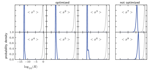
Similarly to the previous section, we will scale the errors as

$$R_{m}=\frac{\tilde{R}_{m}}{\sqrt{\Delta t/N_{S}}}$$ (86)

in order to bring the errors for the unoptimized, randomly sampled vectors close to $1$.

The results in Fig. 5 show that a significant improvement is achieved for all $6$ moments being optimized, with normalized sampling errors reduced to $10^{-12}$, or around twelve orders of magnitude in these examples. Even the non-optimized moments of orders $m=7,8$ have errors reduced to $10^{-5}$, or around five orders.

6.2 Number of iterations and convergence distance

Figure 6: (a) number of iterations taken in the synthetic test for the combined method, $\Delta t=10^{-4}$, $N_{S}=1000$, (b) Relative distance $D$ between the optimized vector $\mathbf{X}^{\mathrm{(opt)}}\left(t+\Delta t\right)$ and the initial approximation $\mathbf{X}_{(0)}\left(t+\Delta t\right)$, and (c) average relative distance $\langle D\rangle$ depending on the number of trajectories $N_{S}$ in the synthetic optimization tests for the individual expansion method, $\Delta t=10^{-4}$. The grey dashed line denotes the slope of a $1/\sqrt{N_{S}}$ dependence.

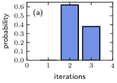
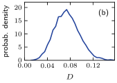
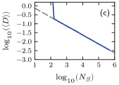
The method requires only a few iterations to converge, as Fig. 6(a) demonstrates.

Next, we calculate the distance of the variance-reduced solution from the original estimate. It is important that this quantity is as small as possible, consistent with the targeted variance reduction, to eliminate systematic errors in higher-order, non-minimized moments. We compute:

$$D=\frac{\|\Delta\mathbf{X}^{\mathrm{(opt)}}-\Delta\mathbf{X}_{(0)}\|}{\|\Delta\mathbf{X}_{(0)}\|}\equiv\frac{\|\mathbf{X}^{\mathrm{(opt)}}\left(t+\Delta t\right)-\mathbf{X}_{(0)}\left(t+\Delta t\right)\|}{\|\mathbf{X}_{(0)}\left(t+\Delta t\right)-\mathbf{X}\left(t\right)\|}$$ (87)

to estimate how far the solution is from the initial approximation. Fig. 6(b) shows that the deviation of the optimized noise from the original is $0.07$ on average, which is of order $1/\sqrt{N_{s}}$ as expected.

Figure 7: (a) Average relative distance $\langle D\rangle$ depending on $\Delta t$ in the synthetic optimization tests for the combined method, with $N_{S}=10^{4.5}$ (dotted yellow line), $N_{S}=10^{5}$ (dash-dotted green line), $N_{S}=10^{5.5}$ (dashed red line) and $N_{S}=10^{6}$ (solid black line). The grey dashed line denotes the least squares fit for the linear part of the $N_{S}=10^{6}$ line and corresponds to the dependence $\langle D\rangle\propto\Delta t^{1.29}$. (b) Average relative distance $\langle D\rangle$ depending on $N_{S}$ in the synthetic optimization tests for the combined method, with $\Delta t=10^{-2.25}$ (dotted yellow line), $\Delta t=10^{-2.5}$ (dash-dotted green line), $\Delta t=10^{-2.75}$ (dashed red line) and $\Delta t=10^{-3}$ (solid black line). The grey dashed line denotes the least squares fit for the linear part of the $\Delta t=10^{-3}$ line and corresponds to the dependence $\langle D\rangle\propto N_{S}^{-0.49}$.

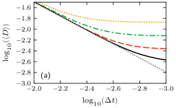
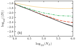
The difference in the orders of $\Delta t$ in the left and the right parts of the target equation (64) leads to the distance $D$ being bounded by a finite value, depending on either $\Delta t$ or $1/N_{S}$. This is unlike the behavior demonstrated by the static optimization in the previous section. Our tests show that for very small $\Delta t$, the asymptotic dependence of $\langle D\rangle$ on $N_{S}$ is $\langle D\rangle\propto 1/\sqrt{N_{S}}$, as shown in Fig. 7(a). Similarly, for very large $N_{S}$ the dependence is $\langle D\rangle\propto\Delta t^{3/2}$, as seen in Fig. 7(b).

This asymptotic error is essentially due to the fact that the moment equations are themselves an expansion in $\Delta t$, leading to a residual truncation error.

Figure 8: Dependence of errors on the number of trajectories $N_{S}$ in the synthetic test for the combined method, $\Delta t=10^{-4}$. Blue solid lines show the average of $R_{m}$ for the optimized vector, grey dotted lines show the average of $R_{m}$ for the initial approximation $\mathbf{X}_{(0)}\left(t+\Delta t\right)$.

Figure 9: Dependence of average scaled errors on $\Delta t$ in the synthetic test for the combined method, $N_{S}=1000$. Blue solid lines show the average of $R_{m}$ for the optimized vector, grey dotted lines show the average of $R_{m}$ for the initial approximation $\mathbf{X}_{(0)}\left(t+\Delta t\right)$.

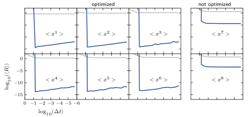
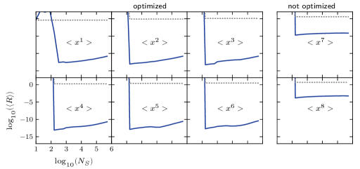
The tests of the dependence on the noise scale ($\Delta t$) show that the method is stable for a wide range of values, but breaks down at larger values of $\mathrm{\Delta}t$ as seen in Fig. 8. The dependence on the number of trajectories in Fig. 9 displays a similar cutoff as seen in the tests of the static POS, in the results of the previous subsection.

6.3 Individual optimization

In this subsection we will use the individual method from Section 5.6, for a similar type of synthetic benchmark. Since the target equations we try to satisfy are different from the previous section, the definition of the error changes to simply

$$\tilde{R}_{m}\left(\mathbf{X}\right)=|e_{m}^{(1)}|+|e_{m}^{(2)}|,$$ (88)

where the vectors $\mathbf{e}^{(1)}$ and $\mathbf{e}^{(2)}$ are defined by Eq. (73).

Similarly to the approach of the previous subsection, we normalize the error as

$$R_{m}=\frac{\tilde{R}_{m}}{\sqrt{\Delta t/N_{S}}}.$$ (89)

Figure 10: Distribution of normalized errors in the synthetic benchmark for the individual method with $\Delta t=0.1$, $N_{S}=1000$. Blue solid lines show the distribution of $R_{m}$ for the optimized vector, grey dotted lines show the distribution of $R_{m}$ for the initial effective noise term $\Delta\mathbf{V}$.

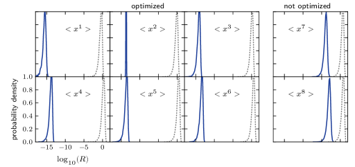
The results in Fig. 10(a) show that a significant improvement is achieved for the first $6$ moments being optimized, with results only limited by the numerical precision. To check that numerical precision was the limiting factor, tests were run with the same method in quadruple precision. This demonstrated that the improvement was indeed limited only by the numerical precision, with errors now as low as $10^{-30}$. The stopping condition must be changed to $\eta=10^{-15}$ to reach this greater numerical precision limit.

6.4 Number of iterations and convergence distance

Figure 11: (a) The number of iterations taken in the synthetic test for the individual method, $\Delta t=0.1$, $N_{S}=1000$. (b) Relative distance $D$ between the optimized vector $\Delta\mathbf{V}^{\mathrm{(opt)}}$ and the initial approximation $\Delta\mathbf{V}$. (c) Average relative distance $\langle D\rangle$ depending on the number of trajectories $N_{S}$ in the synthetic optimization tests for the individual method, $\Delta t=0.1$. The grey dashed line denotes the slope of a $1/\sqrt{N_{S}}$ dependence.

We also calculate the distance

$$D\equiv\frac{\|\Delta\mathbf{V}^{(\mathrm{opt})}-\Delta\mathbf{V}\|}{\|\Delta\mathbf{V}\|}$$ (90)

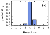
and the number of iterations in our tests. The method also requires only a few iterations to converge, as Fig. 11(a) demonstrates. Fig. 11(b) shows that the deviation of the optimized noise from the original one is small. Unlike the combined method, there is no mismatch between the orders of $\Delta t$ in Eq. (73), and the distance therefore converges as $\langle D\rangle\propto 1/\sqrt{N_{S}}$, as shown in Fig. 11(c).

Figure 12: Dependence of average scaled errors on $\Delta t$ in the synthetic test for the individual method, $N_{S}=1000$. Blue solid lines show the average of $R_{m}$ for the optimized vector, grey dotted lines show the average of $R_{m}$ for the initial approximation $\Delta\mathbf{V}_{(0)}$.

Figure 13: Dependence of errors on the number of trajectories $N_{S}$ in the synthetic test for the expansion method, $\Delta t=0.1$. Blue solid lines show the average of $R_{m}$ for the optimized vector, grey dotted lines show the average of $R_{m}$ for the initial approximation $\Delta\mathbf{V}_{(0)}$.

The tests of the dependence on the noise scale ($\Delta t$) show that this method is exceptionally stable over a wide range of step-size values, as seen in Fig. 12. The dependence on the number of trajectories in Fig. 13 displays a similar cutoff to those seen in the tests of the static POS.

7 Dynamical numerical results

Next, putting all the preliminary results together, tests were performed of complete stochastic differential equation solutions. Although all results demonstrate strong variance reduction, the amount and nature of variance reduction depends on the precise equation, as explained below.

7.1 Linear drift, additive noise

It is instructive to first consider an “ideal” linear SDE for the application of POS, with the target observables being the moments of $x$ as previously. An ideal linear case is one with a linear $a$ and $b$. This is preferred as a first test because the errors from non-optimized moments do not get mixed with the optimized ones, as explained in Section 5.3. In these benchmarks, both the combined and individual methods were used, giving very similar performance overall.

As an example, we used a one-dimensional Ornstein-Uhlenbeck process

$$\mathrm{d}x=\left(f-gx\right)\mathrm{d}t+b\mathrm{d}w,$$ (91)

where $\langle\mathrm{d}w\rangle=0$ and $\langle\mathrm{d}w^{2}\rangle=dt$, and $f$, $g$ and $b$ are constants. It has well-known exact solutions for every moment. Namely, for Gaussian starting conditions the mean is given by:

$$\langle x\rangle=\frac{f}{g}\left(1-e^{-gt}\right)+e^{-gt}\langle x\rangle_{t=0},$$ (92)

and for the variance,

$$\langle\left(x-\langle x\rangle\right)^{2}\rangle=e^{-2gt}\langle\left(x-\langle x\rangle\right)^{2}\rangle_{t=0}+\frac{b^{2}}{2g}\left(1-e^{-2gt}\right),$$ (93)

Higher order central moments are then calculated according to

$$\langle\left(x-\langle x\rangle\right)^{m}\rangle=0,\quad m=3,5,\dots$$ (94)

and:

$$\langle\left(x-\langle x\rangle\right)^{m}\rangle=m!!\langle\left(x-\langle x\rangle\right)^{2}\rangle^{m/2},\quad m=4,6,\dots$$ (95)

Consequently, the raw moments are calculated from the central ones using the recursive formula

$$\langle x^{m}\rangle=\langle\left(x-\langle x\rangle\right)^{m}\rangle-\sum_{p=0}^{m-1}\left(\begin{array}[]{c}m\\ p\end{array}\right)\langle x^{p}\rangle\left(-\langle x\rangle\right)^{m-p}.$$ (96)

We also use cumulants as benchmarks, since these are a commonly used alternative statistical measure to the ordinary moment. The cumulants are calculated from the moments recursively, as

$$\kappa_{m}=\langle x^{m}\rangle-\sum_{p=1}^{m-1}\left(\begin{array}[]{c}m-1\\ p-1\end{array}\right)\kappa_{p}\langle x^{m-p}\rangle.$$ (97)

In our tests we took $f=1$, $g=0.2$, $b=0.5$. At initial times, $x(0)$ is normally distributed with mean $0.5$ and standard deviation $0.1$. We pre-optimized the starting distributions using the static method from Section 3.4 in order to satisfy the requirements of POS methods.

7.2 Cumulant and moment variance reduction

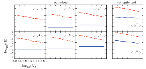
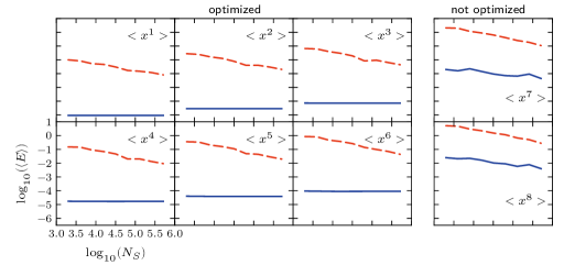
For our tests, we compare the deviations — due to sampling errors — from the exact solution in the first $8$ moments and first $8$ cumulants of $x$ at $t=1$ for the POS integrator. We use both combined and individual methods, with a reference SDE solver having the same number of samples, for comparison. The latter uses the same integration method (explicit Euler) and the same number of trajectories as POS. We set up POS to optimize the first $6$ moments, so that we could look at the behavior of both optimized and non-optimized moments.

Figure 14: Linear SDE case with $M=6$ optimized moments, showing the difference of the first $8$ moments from the exact solution at $t=1$ for the POS integrator using the combined method (solid blue lines) and a reference explicit Euler integrator (dashed red lines), with identical numbers of trajectories and samples, averaged over $8$ tests. Both integrators use $N_{T}=8\times 10^{4}$ time steps.

Figure 15: Linear SDE case with $M=6$ optimized moments, showing the difference of the first $8$ moments from the exact solution at $t=1$ for the POS integrator using the individual method (solid blue lines) and a reference explicit Euler integrator (dashed red lines), with identical numbers of trajectories and samples, averaged over $8$ tests. Both integrators use $N_{T}=8\times 10^{4}$ time steps.

In Figs. 14 and 15 we plotted the error in the first moments

$$E\left[\langle x^{m}\rangle\right]=\left|\langle x^{m}\rangle-\langle x^{m}\rangle^{(\mathrm{exact})}\right|$$ (98)

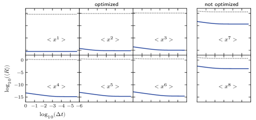
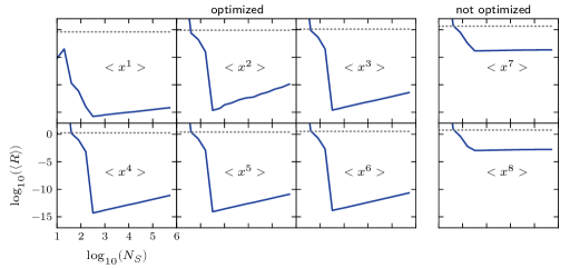
for the reference and the two POS integrators, averaged over $8$ independent tests. In case of the POS methods the error is dominated by the time step error $\epsilon_{T}$, while the error for the reference integrator decreases proportional to $1/\sqrt{N_{S}}$. One can see that the POS error is significantly decreased even for the moments that were not directly optimized. The error improvement is largest for the individual method, but is still several orders of magnitude even for the simpler combined method. For the remaining graphs we will mostly focus on the individual method which give better results, to minimize the number of graphs, as both have similar general behavior.

Figure 16: Linear SDE case with $M=6$ optimized moments, showing the difference of the first $8$ cumulants from the exact solution at $t=1$ for the POS integrator using the individual method (solid blue lines) and a reference explicit Euler integrator (dashed red lines), with identical numbers of trajectories and samples, averaged over $8$ tests. Both integrators use $N_{T}=8\times 10^{4}$ time steps.

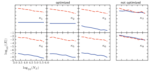
The general behavior in the linear case can be understood better if we plot the errors in the cumulants $E\left[\kappa_{p}\right]$ instead, as in Fig. 16. It shows that the error in the first $6$ cumulants is greatly reduced, while the non-optimized cumulants stay roughly the same. In Fig. 15, $7$-th and $8$-th moments, while not being optimized directly, still depend on the lower cumulants, and thus benefit from their reduced error. This behavior is caused by the fact that in a linear SDE, cumulants of different orders are not coupled with each other; however moments are coupled, leading to the observed error performance.

7.3 Nonlinear drift, additive noise

As an example of a real-world, nonlinear SDE we can apply the POS method to, we take an equation with a nonlinear drift term and additive noise:

$$\mathrm{d}x=\left(x-x^{3}\right)\mathrm{d}t+\mathrm{d}w,$$ (99)

where $\langle\mathrm{d}w\rangle=0$ and $\langle\mathrm{d}w^{2}\rangle=1$. This is similar to a known case where moment hierarchy methods fail to give correct results [18].

For large times $t$, Eq. (99) converges to a steady-state solution. For any given observable $\left\langle f\left(x\right)\right\rangle$, we can find its steady-state value using the formula

$$\left\langle f\left(x\right)\right\rangle_{ss}=\frac{\int_{-\infty}^{\infty}f\left(x\right)e^{x^{2}-\frac{1}{2}x^{4}}\mathrm{d}x}{\int_{-\infty}^{\infty}e^{x^{2}-\frac{1}{2}x^{4}}\mathrm{d}x}.$$ (100)

We initialize our ensemble with normally-distributed numbers with mean $0$ and standard deviation $\frac{1}{\sqrt{2}}$ and integrate Eq. (99) using a combined POS-method as well as an unoptimized Ito-Euler method until $t=25$ and then compare with the steady-state values. The POS-optimized integration includes an initial static optimization. Integrating until $t=25$ ensures that Eq. (99) predicts observables sufficiently close to the steady-state values. We assume that after some integration time, the time evolution of the observables will be dominated by a transient which is exponentially converging to the steady-state solution. A least-squares fit of the time-evolution of the $8$’th moment is in excellent agreement with the time-evolution resulting from our simulations. From the fitting parameters, we can read off a decay of more that $50$ mean lifetimes at $t=25$. We conclude that the deviation from the steady-state value due to finite integration time is negligible compared to sampling errors. As in the previous section, we plot the first $8$ moments and first $8$ cumulants of $x$ at $t=25$, but we optimize only the first $6$ moments when the POS is used. In order to show the behaviour of non-polynomial observables, we also plot the exponential and absolute value of $x$.

Figure 17: Nonlinear SDE case with $M=6$ optimized moments, showing the difference of the first $8$ moments, as well as the exponential and absolute value function from the steady-state solution at $t=25$ for the POS integrator using the combined method (solid blue lines). We also include the errors in an explicit Euler integrator (solid red lines), with identical numbers of trajectories and samples, for comparison. Both integrators use $N_{T}=12.5\times 10^{3}$ time steps. The dash-dotted grey line shows the slope for $\propto N_{S}^{-1/2}$.

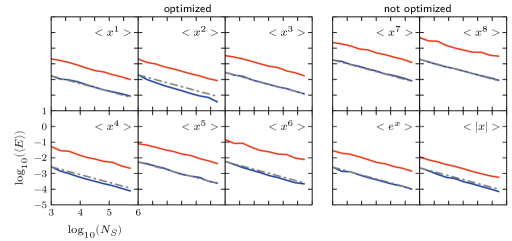
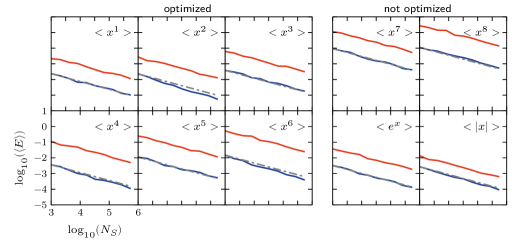
In Fig. 17 we are plotting differences from the accurate solution for the first $8$ moments:

$$E\left[\langle x^{m}\rangle\right]=\left|\langle x^{m}\rangle-\langle x^{m}\rangle_{ss}\right|$$ (101)

as well as for the exponential and absolute value function defined analogously to Eq. (101) averaged over $120$ independent test runs for the POS integration and $600$ runs for the reference integration.

The POS integrator consistently outperforms the reference integrator, with errors reduced by a factor of $10-100$.

A sampling error reduction of this order of magnitude requires $10^{2}-10^{4}$ times more samples using standard integrators.

Figure 18: Nonlinear SDE case, showing the difference of the first $8$ cumulants from the steady-state values at $t=25$ for the POS integrator using the combined method (solid blue lines) and a reference explicit Euler integrator (dashed red lines). Both integrators use $N_{T}=12.5\times 10^{3}$ time steps. The dash-dotted grey lines shows the slope for $\propto N_{S}^{-1/2}$.

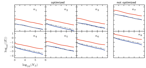
In Fig. 18 we show results for the cumulants in the nonlinear case, for completeness. Unlike the linear case, where the improvement was confined to only the explicitly optimized cumulants, we see that in the nonlinear case even the non-optimized cumulants are optimized as well. This is because the nonlinear equations couple all cumulants with each other. The results show that POS results in dependency slightly better than $N_{S}^{-1/2}$ for the even cumulants. This is an interesting and noteworthy results though we don’t have an explanation for it yet.

In a separate analysis, we have integrated Eq. (99) until $t=4$ with a time-step of $\Delta t=4\times 10^{-4}$ using both the combined and the individual POS-method as well as an explicit Ito-Euler reference method. We have compared the values of the first $8$ consecutive moments and cumulants with that of a regular SDE integrator with $N_{T}=8\times 10^{4}$ time steps and $N_{S}=10^{9}$ trajectories, using a central difference integration method [24]. The large number of trajectories for the regular SDE integrator ensured that we obtained a sufficiently accurate estimate for the true value of the moments and cumulants at $t=4$. The comparison showed that individual POS method performed very similarly to the combined POS method, resulting in a similarly good accuracy improvement. In the interest of space, we are limiting our results to the combined POS method from now on.

7.4 Irregular drift, additive noise

We now investigate the properties of an SDE whose functional behaviour is not a regular polynomial. We chose the SDE

$$\mathrm{d}x=x\left(1-\left|x\right|\right)\mathrm{d}t+\mathrm{d}w,$$ (102)

where $\langle\mathrm{d}w\rangle=0$ and $\langle\mathrm{d}w^{2}\rangle=1$.

We can obtain the steady-state solutions for a given observable $\left\langle f\left(x\right)\right\rangle$ via

$$\left\langle f\left(x\right)\right\rangle_{ss}=\frac{\int_{-\infty}^{\infty}f\left(x\right)e^{x^{2}-\frac{2}{3}\left|x\right|x^{2}}\mathrm{d}x}{\int_{-\infty}^{\infty}e^{x^{2}-\frac{2}{3}\left|x\right|x^{2}}\mathrm{d}x}.$$ (103)

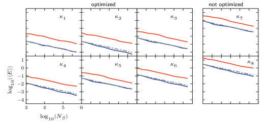
We run a simulation identical to the one in Section 7.3, where we replace the SDE by Eq. (102). An analysis analogous to that in Section 7.3 reveals an equally good convergence to the steady-state values at $t=25$. The results given in Fig. 19 show that the overall performance of POS for the non-regular SDE is very similar to that for the nonlinear SDE studied in Section 7.3. Despite the fact that Eq. (102) is non-regular, we observe virtually the same rate of improvement through POS as we did for the regular SDE.

Figure 19: Nonlinear SDE case, showing the difference of the first $8$ moments, the exponential and absolute value function from the steady-state solution at $t=25$ for the POS integrator using the combined method (solid blue lines) and a reference explicit Euler integrator (solid red lines). Both integrators use $N_{T}=12.5\times 10^{3}$ time steps. The dash-dotted grey line shows the slope for $\propto N_{S}^{-1/2}$.

Figure 20: Nonlinear SDE case, showing the difference of the first $8$ cumulants from the accurate solution at $t=25$ for the POS integrator using the individual method (solid blue lines) and a reference explicit Euler integrator (solid red lines). Both integrators use $N_{T}=12.5\times 10^{3}$ time steps. The dash-dotted grey line shows the slope for $\propto N_{S}^{-1/2}$ .

8 Two-dimensional case

Finally, to demonstrate that POS can be applied to SDE’s with dimension higher than $1$, we briefly consider the so-called laser equation. This is a simplified model for the single-mode quantum statistics in a laser system. Although it can be written as a single complex equation, it is an example of an SDE with dimension higher than one in real variables. We consider

$$da=\left(1-\left|a\right|^{2}\right)a\ dt+b\ dW_{c},$$ (104)

where both $a$ and $dW_{c}$ are complex-valued. The noise obeys $\left\langle dW_{c}dW_{c}^{*}\right\rangle=2dt$. Here $a$ is proportional to the mode amplitude, and $b$ is a real-valued parameter that depends on the steady-state photon number of the laser mode [25]. By treating the real and imaginary parts of $a$ as separate variables, Eq. (104) constitutes a two-dimensional real-valued SDE.

The scaled photon number $n$ is given by $n=\left|a\right|^{2}$. A simple calculation reveals the steady-state value for $n$ to be

$$n_{ss}=1+\sqrt{\frac{2}{\pi}}\frac{b}{\exp\left[1/\left(2b^{2}\right)\right]\left[1+\text{erf}\left(1/\left(\sqrt{2}b\right)\right)\right]}\,.$$ (105)

Using $N_{S}=131072$ trajectories for the real and imaginary part $\Re\left\{a\right\}$ and $\Im\left\{a\right\}$, resulting in $N_{S}=262144$ trajectories in total, we initialize the ensemble with normally-distributed numbers with mean $0$ and standard deviation $\frac{1}{\sqrt{2}}$ for $\Re\left\{a\right\}$ and $\Im\left\{a\right\}$ and carry out a POS-optimized integration using the combined method as well as an explicit Ito-Euler reference integration with an integration time of $t=25$. An analysis similar to that in Sections 7.3 and 7.4 reveals an equally good convergence to the steady-state at $t=25$. We then compare the value of $n=\left|a\right|^{2}$ at $t=25$ with the steady-state value.

8.1 Error in the equilibrium photon number

We are optimizing (constraining) every moment and cross-moment for the real and imaginary part of $a$ up to order 4. In other words, we are optimizing the first 4 consecutive moments of $\Re\left\{a\right\}$, of $\Im\left\{a\right\}$ and cross-moments of the form $\Re\left\{a\right\}^{n}\Im\left\{a\right\}^{m}$, with a combined power $n+m$ not greater than 4. This results in a total of 18 constrained moments. The POS optimization includes the optimization of the initial trajectories.

We vary the parameter $b$ over a range from $1\cdot 10^{-2}$ to $10.24$ in $11$ steps. As in Sections 7.3 and 7.4 we average over $120$ independent test runs for the POS integration and $600$ runs for the reference integration.

As a typical physical example of a scientifically important quantity in a stochastic calculation, Fig. 21 shows the error in calculating $n_{s}$, the equilibrium photon number in the laser cavity. Here we use the combined Ito POS method (blue line), and a non-optimized stochastic integration (red line) for the laser equation for different values of $b$.

Figure 21: Accuracy of the scaled photon number $n_{s}$ for the laser equation using a reference explicit Euler integrator (red line) and a POS-optimized integration (blue line) as a function of the parameter $b$. Both integrators use $N_{T}=12.5\times 10^{3}$ time steps.

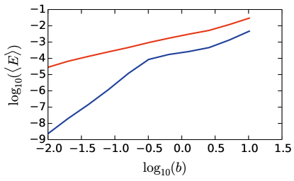
This example shows that POS can be successfully used to improve the accuracy of complex-valued SDEs and, more generally speaking, real-valued multivariate SDEs by several orders of magnitude.

9 Conclusions

In summary, we have proposed and implemented a novel variance reduction technique for solving stochastic differential equations, using parallel optimized sampling. The essential feature is that it unifies moment hierarchy and independent stochastic methods.

A finite moment hierarchy condition is imposed as a nonlinear constraint on the random noises generated at each step in the integration. This gives a dramatic reduction in sampling error for all moments calculated. In the case of linear equations, we find that the low order moments have sampling errors reduced to machine accuracy. While higher order moments also have their errors reduced, the higher order cumulants are not affected.

For nonlinear equations, the error reduction is not as large, but it occurs over all moments and cumulants studied, even including the non-optimized cumulants of higher order than the optimization limit. We emphasize that the proposed algorithms have a general applicability to all types of stochastic equations, and can be extended in principle to higher order methods as well as the simple Euler integration treated here.

References

- [1] P. Langevin, Sur la théorie du mouvement brownien, C. R. Acad. Sci. (Paris) 146 (1908) 530–533.
- [2] D. S. Lemons, Paul Langevin’s 1908 paper “On the Theory of Brownian Motion” [“Sur la théorie du mouvement brownien,” C. R. Acad. Sci. (Paris) 146, 530–533 (1908)], Am. J. Phys. 65 (11) (1997) 1079. doi:10.1119/1.18725.
- [3] G. Uhlenbeck, L. Ornstein, On the Theory of the Brownian Motion, Phys. Rev. 36 (5) (1930) 823–841. doi:10.1103/PhysRev.36.823.
- [4] L. Arnold, Stochastic differential equations: theory and applications, reprint Edition, Folens Publishers, 1992.
- [5] H. Risken, The Fokker-Planck Equation, 2nd Edition, Springer-Verlag, Berlin, 1996.
- [6] C. W. Gardiner, Handbook of Stochastic Methods, 2nd Edition, Springer-Verlag, Berlin, 1985.
- [7] I. Karatzas, S. Shreve, Brownian motion and stochastic calculus, 2nd Edition, Springer, 1991.
- [8] N. G. Van Kampen, Stochastic Processes in Physics and Chemistry, 3rd Edition, North Holland, 2007.
- [9] P. Glasserman, Monte Carlo Methods in Financial Engineering, reprint Edition, Springer, 2010.
- [10] G. N. Mil’shtein, Approximate Integration of Stochastic Differential Equations, Theor. Probab. Appl. 19 (3) (1975) 557–562. doi:10.1137/1119062.
- [11] D. L. Ermak, H. Buckholz, Numerical integration of the Langevin equation: Monte Carlo simulation, J. Comput. Phys. 35 (2) (1980) 169–182. doi:10.1016/0021-9991(80)90084-4.
- [12] D. Talay, L. Tubaro, Expansion of the global error for numerical schemes solving stochastic differential equations, Stoch. Anal. Appl. 8 (4) (2007) 483–509. doi:10.1080/07362999008809220.
- [13] P. E. Kloeden, E. Platen, Numerical Solution of Stochastic Differential Equations, Springer-Verlag, Berlin, 1992.
- [14] K. Burrage, T. Tian, A note on the stability properties of the euler methods for solving stochastic differential equations, New Zeal. J. Math. 29 (2) (2000) 115–127.
- [15] D. J. Higham, An Algorithmic Introduction to Numerical Simulation of Stochastic Differential Equations, SIAM Rev. 43 (3) (2001) 525–546. doi:10.1137/S0036144500378302.
- [16] W. J. Morokoff, R. E. Caflisch, Quasi-Monte Carlo Integration, J. Comput. Phys. 122 (2) (1995) 218–230. doi:10.1006/jcph.1995.1209.
- [17] M. B. Giles, Multilevel Monte Carlo Path Simulation, Oper. Res. 56 (3) (2008) 607–617. doi:10.1287/opre.1070.0496.
- [18] M. Morillo, J. Gómez-Ordóñez, J. M. Casado, Checking the Validity of Truncating the Cumulant Hierarchy Description of a Small System, in: R. Carretero-González, J. Cuevas-Maraver, D. Frantzeskakis, N. Karachalios, P. Kevrekidis, F. Palmero-Acebedo (Eds.), Localized Excitations in Nonlinear Complex Systems, Vol. 7 of Nonlinear Systems and Complexity, Springer International Publishing, 2014, pp. 377–387. doi:10.1007/978-3-319-02057-0.
- [19] P. Hänggi, P. Talkner, A remark on truncation schemes of cumulant hierarchies, J. Stat. Phys. 22 (1) (1980) 65–67. doi:10.1007/BF01007988.
- [20] A. Gilchrist, C. W. Gardiner, P. D. Drummond, Positive P representation: Application and validity, Phys. Rev. A 55 (4) (1997) 3014–3032. doi:10.1103/PhysRevA.55.3014.
- [21] P. P. Deuar, P. D. Drummond, Gauge P representations for quantum-dynamical problems: Removal of boundary terms, Phys. Rev. A 66 (3) (2002) 033812. doi:10.1103/PhysRevA.66.033812.
- [22] T. Aimi, M. Imada, Gaussian-Basis Monte Carlo Method for Numerical Study on Ground States of Itinerant and Strongly Correlated Electron Systems, J. Phys. Soc. Jpn. 76 (8) (2007) 084709. doi:10.1143/JPSJ.76.084709.
-
[23]
P. L’Ecuyer, Efficiency
Improvement and Variance Reduction, in: Proceedings of the 26th Conference
on Winter Simulation, Society for Computer Simulation International, San
Diego, CA, USA, 1994, pp. 122–132.
URL http://dl.acm.org/citation.cfm?id=193201.193994 - [24] M. J. Werner, P. D. Drummond, Robust Algorithms for Solving Stochastic Partial Differential Equations, J. Comput. Phys. 132 (2) (1997) 312–326. doi:10.1006/jcph.1996.5638.
[25]
P. D. Drummond, M. Hillery,
The
Quantum Theory of Nonlinear Optics, Cambridge University Press, 2014.
URL http://www.cambridge.org/us/academic/subjects/physics/optics-optoelectronics-and-photonics/quantum-theory-nonlinear-optics?format=HB