Ranking the importance of nuclear reactions for activation and transmutation events

Abstract

Pathways-reduced analysis is one of the techniques used by the Fispact-II nuclear activation and transmutation software to study the sensitivity of the computed inventories to uncertainty in reaction cross-sections. Although deciding which pathways are most important is very helpful in for example determining which nuclear data would benefit from further refinement, pathways-reduced analysis need not necessarily define the most critical reaction, since one reaction may contribute to several different pathways. This work examines three different techniques for ranking reactions in their order of importance for determining the final inventory, comparing the pathways-based metric (PBM), the direct method and one based on the Pearson correlation coefficient. Reasons why the PBM is to be preferred are presented.

1 Introduction

Fispact-II is a software suite for the analysis of nuclear activation and transmutation events of all kinds [1]. The present work focuses on its use in sensitivity studies of nuclear inventory calculations; these employ the Bateman model for the evolution of the inventory of a target subject to irradiation by an imposed flux of projectile particles, always neutrons herein. In ref [2] it was established that the pathways-reduced approach [3, 4] to such studies, almost invariably gives very close agreement with Monte-Carlo sensitivities computed using full Bateman, i.e. accounting for all nuclides and pathways. Pathways-reduced models are, following Eastwood and Morgan [3], identified by a graph-based approach which determines the key reaction pathways determining the inventory at a given time and eliminates from consideration those nuclides which do not lie on this reduced set of pathways.

The pathways-reduced metric is a sensitivity method in the respect that implicitly it selects a set of the most important nuclide reactions. A wide range of other sensitivity methods has been used by the nuclear industry as shown by literature reviews by Helton et al [5], see also Cacuci and Ionescu-Bujor [6, 7]. Indeed, sensitivity analyses are available as part of nuclear industry software packages such as for example DAKOTA [8] and SCALE [9]. General purpose sensitivity software is also available, such as OpenCossan [10].

A key input to most techniques considered herein is an estimate of the uncertainty in the reaction cross-section. The determination of such uncertainties is a challenging subject in its own right, hence it is important to examine techniques that can identify which reactions most require further examination. The present work represents a comparison of three different techniques that exploit the pathways-based reduction for the nuclear activation problem.

Fispact-II can access uncertainty data, typically the standard deviation, for the vast majority of reaction cross-sections in the EASY-II database [11], however no information is currently passed concerning pure decay reactions. This reflects the fact that half-lives are often very accurately known. There are other reactions in the database for which a value of zero uncertainty is found, usually indicating that no information is available. There are thus difficulties in making the comparison, the implications of which are discussed in Section 2.4.

To proceed further with this introduction, it is efficient to introduce the time evolution (rate or Bateman equation) for a nuclear inventory $X$

$$\frac{dX}{dt}=\mathsf{A}X$$ (1)

where $X$ is the vector of nuclide numbers, and $\mathsf{A}$ is the matrix of nuclear interaction coefficients for both induced reactions and spontaneous decays. Note that one coefficient $A_{ij}$ of $\sf{A}$ may represent several different nuclear reactions, since the equation involves an average over a spectrum of energies (of neutrons in the present work, although other elementary particles may be considered in general). Hence the term ‘interaction’ is used to cover all effects generating nuclide $i$ as the child of parent $j$. It is worth noting that although $i$ precedes $j$ alphabetically, reactions throughout this work will except for the $A_{ij}$ be described in parent-child order. In general, the coefficients $A_{ij}$ may change with time as the incident neutron flux changes.

All the techniques for ranking the interactions $A_{ij}$ are most easily understood in the context of a single constant irradiation in the time interval $(0,t_{f})$, producing an inventory $X(t_{f})$. Different aspects of the inventory, such as heat production or kerma, may be studied using Fispact-II, but for illustrative purposes it is sufficient to consider only the total activity

$$Q=\sum_{k}\lambda_{k}X_{k}(t_{f})$$ (2)

where $\lambda_{k}$ is the decay rate of the nuclide $X_{k}$; $\lambda_{k}$ is zero for stable nuclides and $\lambda_{k}=\log_{e}2/\tau_{k}$ for unstable ones, where $\tau_{k}$ is the half-life. Although attention focuses here on Fispact-II, the Bateman approach is standard in that most packages with a claim to generality, not only DAKOTA and SCALE in the U.S. but also ANSWERS [12] with FISPIN in the U.K., include solvers for the problem. The pathways-based analysis technique studied here could in principle be implemented in any of these codes.

The three different ranking techniques are described in the next Section 2. Apart from the use of pathways-based reduction, there is novelty in the calculation of the direct sensitivity, in that the matrix Fréchet derivative is used in its computation, see Appendix, rather than the more usual decoupled direct method DDM of Dunker [13]. The application of the techniques to the wide range of test cases first introduced in ref [2] is illustrated in Section 3. Lastly Section 4 compares the utility of the different techniques.

2 Sensitivity Measures

2.1 Pathways Based Metric

The Pathways Based Metric (PBM) is calculated quite simply from the output of the pathways-reduced approach, which includes a listing of each pathway and its percentage contribution to the active nuclide at its termination. For a given interaction $A_{ij}$, all the number $N_{p}$ of pathways upon which it lies are identified and the PBM calculated as

$$S_{PBM}^{ij}=\sum_{k=1}^{N_{p}}p_{l}\lambda_{t}X_{t}I_{kl}$$ (3)

where $p_{l}$ is the fractional contribution of pathway $l$ to the number of atoms $X_{t}$ (evaluated at time $t_{f}$) in the inventory with decay rate $\lambda_{t}$ and the indicator matrix $I_{kl}=1$ or $0$ depending whether or not a reaction contributing to the interaction lies on the pathway.

Figure 1 illustrates how the definition works in a simplified case where irradiation of an initial sample consisting of $X_{1}$ atoms of nuclide $1$ and $X_{2}$ atoms of nuclide $2$ produces an inventory containing numbers $X_{5}$ and $X_{6}$ of radioactive nuclides $5$ and $6$ respectively, with $3$ important pathways. The first pathway contributes $p_{1}X_{5}$ atoms and the third $p_{3}X_{5}$ atoms of nuclide $5$. (Supposing that other pathways are unimportant, $p_{1}+p_{3}\approx 1$ and $p_{2}\approx 1$.) The sensitivity of the inventory to the reaction with coefficient $A_{32}$ (large arrowheads in Figure 1), is then

$$S_{PBM}^{32}=p_{1}\lambda_{5}X_{5}+p_{2}\lambda_{6}X_{6}$$ (4)

where $\lambda_{5}$ is the decay rate of nuclide $5$ etc.

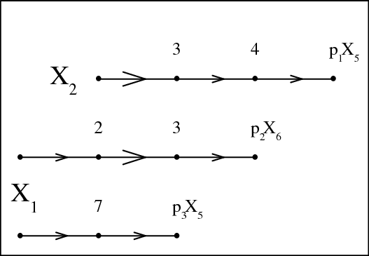
Figure 1: Example illustrating how the Pathways Based Metric $S_{PBM}$ is calculated when the three pathways shown are highlighted by the pathways-reduced analysis. The pathways are numbered in order $1$, $2$ and $3$ from the top. Pathway $1$ starts with nuclide $2$ and generates via a sequence of reactions involving nuclides $3$ and $4$, $p_{1}X_{5}$ atoms of nuclide $5$, whereas the other pathways begin with nuclide $1$ and generate nuclides $6$ and $5$ respectively. The larger arrowheads indicate reactions with the coefficient of interest $A_{32}$.

This technique required special modification to Fispact-II for its implementation, which was facilitated by the object-oriented design of the Fortran-95 code. For the purposes of initial investigation, the loops which are identified by the graph-based approach used by Fispact-II are ignored.

2.2 Direct Method

The Direct Method (DM) works directly with the tensor describing the rate of variation of the nuclide $X_{k}$ with respect to nuclear reaction coefficients. For initial investigative purposes it is sufficient to consider the partial derivative with respect to $A_{ij}$. Differentiating Eq. (1) with $(i,j)$ regarded as fixed, gives

$$\frac{d}{dt}\left(\frac{\partial X}{\partial A_{ij}}\right)=A\frac{\partial X}{\partial A_{ij}}+\frac{\partial A}{\partial A_{ij}}X$$ (5)

If the sensitivity of the total activity is required, then using Eq. (2), this is

$$S_{DM}^{ij}=\sum_{k}\lambda_{k}\frac{\partial X_{k}(t_{f})}{\partial A_{ij}}$$ (6)

In the decoupled direct method, Eq. (5) is solved for $\partial X_{k}/\partial A_{ij}$ using a method which exploits the sparseness of $\partial A/\partial A_{ij}=\delta_{ij}$ in the present context. However, it is also possible to express $S_{DM}$ in terms of the matrix Fréchet derivative as explained in the Appendix, viz.

$$S_{FDM}^{ij}(t_{f})=t_{f}\sum_{k}\lambda_{k}L_{\exp}(t_{f}\mathsf{A},\mathsf{E}_{ij})X(0)$$ (7)

where $L_{\exp}$ is the matrix Fréchet derivative as defined in the Appendix where $\mathsf{E}_{ij}$ is also defined. Eq. (7) defines the Fréchet direct method. Similarly to the PBM, this technique required modification of Fispact-II to output the matrix $\mathsf{A}$ in a format suitable for input to MATLAB [14].

2.3 Pearson Derived Method

The Pearson technique for ranking sensitivities starts with the definition of the Pearson product-moment correlation coefficient for a set of $N_{s}$ samples $\{(A_{s},Q_{s}):s=1,\ldots,N_{s}\}$, viz.

$$r=\frac{\sum_{s}(Q_{s}-\bar{Q})(A_{s}-\bar{A})}{(N_{s}-1)\Delta Q\Delta A}$$ (8)

where the suffix $ij$ on $r$ and $A$ is to be understood, overbar denotes average and $\Delta$ denotes the standard deviation of the distribution so that for example

$$\bar{Q} = \frac{1}{N_{s}}\sum_{s=1}^{N_{s}}Q_{s}$$ (9)

$$\Delta Q = \sqrt{\frac{1}{(N_{s}-1)}\sum_{s=1}^{N_{s}}[(Q_{s})^{2}-\bar{Q}^{2}]}$$ (10)

The coefficient $r_{ij}$ is by definition always less than or equal to one, and a magnitude of $r$ close to one indicates strong linear correlation.

However, it is the proportionality constant corresponding to $\partial Q/\partial A_{ij}$ that is of initial interest. It is worth cautioning that although the definition implicitly implies a linear relation, there is no guarantee of this. However, in order to proceed, linearity will be assumed, viz.

$$Q-\bar{Q}=\tilde{r}(A-\bar{A})$$ (11)

and substituting in Eq. (8), it follows that

$$S_{PRD}=\tilde{r}_{ij}=r_{ij}\left(\frac{\Delta Q}{\Delta A}\right)$$ (12)

It follows that the output of the Monte-Carlo sensitivity calculations may be used to rank the different interactions by computing $r_{ij}/\Delta A$ (note that $\Delta Q$ is the same for all the $A_{ij}$ variations in the standard approach described in ref [2]).

The calculation of the Pearson coefficient $r$ is well-known to be sensitive to round-off error. To avoid modifying the software, the coefficient is computed using output values from Fispact-II given only to $6$ significant figures by default. This accuracy is the maximum that can be expected from the numerical integration of the rate equation which is is constrained to an accuracy of one part in a million. It was found that splitting the separate contributions of $A_{s}$ and $\bar{A}$ to Eq. (8) led to unacceptable cancellation due to round-off effects (although it was verified that round-off was not a similar issue for $Q_{s}$ and $\bar{Q}$).

2.4 Comments upon the Different Metrics

The main distinction between the PBM and the other two measures is that the pathways-based method is ‘global’, capturing the whole variation of the inventory as parameters are varied, although having the disadvantage that it cannot measure sensitivity to diagonal entries of $\sf{A}$. The other two techniques are more local, indeed the DM returns directly only a coefficient at the mean of the distribution of $Q$. The Pearson method is somewhere in-between, using global variations, but making a local linear assumption about the mean. This complicates the comparison in the next Section 3.

The principal comment to be made concerning the comparison is that, corresponding to the lack of sensitivity to element $A_{ij}$ when it is zero due an absence of interaction between nuclides $i$ and $j$, a large sensitivity in the local sense may be inconsequential for the total activity $Q$ if the corresponding $A_{ij}$ is relatively very small. However, the two more local estimates (Eq. (6) and Eq. (12)) for $\partial Q/\partial A_{ij}$ should be directly comparable.

Main interest attaches to global measures such as $S_{PBM}$. The FDM approach may be used to produce an equivalent ranking by scaling by the estimated error in the coefficient, viz.

$$S_{FDS}^{ij}=S_{FDM}^{ij}\cdot\left(\frac{\epsilon_{ij}}{100}\right)\cdot\bar{A}_{ij}$$ (13)

where $\epsilon_{ij}$ is the percentage error in the distribution of the coefficient $A_{ij}$. Fispact-II returns both  $\epsilon_{ij}$ and $\bar{A}_{ij}$ by combining the uncertainties in the reaction coefficients corresponding to $A_{ij}$.

From Eq. (12), a ranking based on the Pearson coefficient $r$ should also be comparable to $S_{PBM}$, if it is scaled similarly, viz.

$$S_{PRS}^{ij}=r_{ij}\cdot\left(\frac{\epsilon_{ij}}{100}\right)\cdot\left(\frac{\bar{A}_{ij}}{\Delta A_{ij}}\right)$$ (14)

In practice it is found that $S_{PRS}^{ij}\approx r_{ij}$.

Note that for interactions for which no uncertainty information is available, a Pearson coefficient cannot be computed, nor is $S_{FDS}$ useful. The coefficient $S_{PBM}$ may be non-zero, but this relies on the interaction’s lying on a pathway important for other reasons. Interactions without accompanying uncertainty information will therefore largely have to be ignored in this work.

3 Sensitivity Calculations

3.1 Details of Cases

The test cases are taken from ref [2] and involve several different nuclide mixtures designed to be indicative of a wide range of activation problems, see Table 1. As indicated, all but one of the mixtures consisted of $1$ kg of material subject to a neutron flux of $10^{15}$ $cm^{-2}s^{-1}$, for a year, without any cooling period.

The mixtures are used in six test cases, with the Alloy case extended to include a cooling phase. Each test case is run using the full TENDL 2013 data from the EASY-II database [11] with pathways analysis to identify the important reactions, the numbers of which are listed in Table 2. As in ref [2], Monte-Carlo solution of the reduced problem, investigating the distributions of the important reaction rates specified in the newer database, was then performed in the sequence of increasing sample size per reaction, $N_{x}=10,\;40,\;160,\;\ldots$ up to the maximum value specified in the table. Indications from ref [2] and work which may be published elsewhere indicate that the pathways-reduced results agree to at least two (and often three) significant figures with those obtained by sampling the full problem, at less than a thousandth of the computational cost. As might be expected from the large maximum number of samples $N_{s}$ employed, the distributions of reaction rates actually sampled usually agree in the mean to $4$ significant figures with the nominal database values.

Table 1: Test cases. Each consists of numbers of atoms of the listed elements with their natural abundances of nuclides, given as percentages by mass of the whole.

Test	Constituents of Mixture	Sample	Irradiation	Cooling	Neutron flux
Label		Mass	Period	Period	cm-2s-1
Alloy	Fe $40.0$ : Ni $20.0$ : Cr $20.0$ : Mn $20.0$	$1$ kg	$1$ yr	0	$10^{15}$
Alloy+c	Fe $40.0$ : Ni $20.0$ : Cr $20.0$ : Mn $20.0$	$1$ kg	$1$ yr	$1$ yr	$10^{15}$
Fe	Fe	$1$ kg	$2.5$ yr	0	$10^{15}$
LiMix	Li $40.0$ : Be $30.0$ : O $30.0$	$1$ kg	$1$ yr	0	$10^{15}$
WMix	W $20.0$ : Re $20.0$ : Ir $20.0$ : Bi $20.0$ : Pb $20.0$	$1$ kg	$1$ yr	0	$10^{15}$
Y2O3	Y $78.74$ : O $21.26$	$1$ g	$300$ s	0	$1.116\times 10^{10}$

Table 2: Test cases statistics. Monte-Carlo sampling by Fispact-II has a sample size determined by the number of reactions examined.

Test	$I$, Reactions	Matrix	Max. $N_{x}$, Samples	$N_{s}$, Total
Label	Examined	$\mathsf{A}$ Size	per Reaction	Sample
Alloy	$84$	$51$	$640$	$53\,760$
Alloy+c	$50$	$38$	$640$	$32\,000$
Fe	$27$	$24$	$640$	$17\,280$
LiMix	$17$	$21$	$640$	$10\,880$
WMix	$71$	$63$	$640$	$45\,440$
Y2O3	$13$	$16$	$2\,560$	$33\,280$

3.2 Results

This section presents results for each of the test cases in turn, in the alphabetic order specified in Table 1. Attention is drawn to the fact that the Y2O3 case is the simplest in terms of pathways, and contains extra explanation.

For each test case there is a table of sensitivity rankings ordered by Fréchet derivative amplitude and a graph of rankings ordered by $S_{PBM}$. The table enables a larger range of interactions to be compared, since the graphs become hard to interpret once the number of plotted interactions exceeds about ten. Note the convention (except for the Y2O3 case) that all three methods must provide a ranking for the comparison to be plotted. So in the figures the ten highest-ranked cases plotted may include reactions significantly smaller in importance than the tenth.

A general feature of all graphs comparing rankings by the different techniques is the symmetry about the mid-line labelled $PBM$. The appearance of “$V$” and “$\Lambda$” patterns indicates that although the more local measures may not agree with $S_{PBM}$, they do themselves correlate well.

For three of the test cases, Alloy+c in Section 3.2.2, WMix in Section 3.2.5 and Y2O3 in Section 3.2.6, further results of analysis are presented to help understand the effect of sampling and round-off on the calculation of $S_{PRS}$. In addition, a table of sensitivity rankings ordered by $S_{PBM}$ and a graph of rankings ordered by Fréchet derivative also appear in these two sections. (This information is omitted from the other four sections Section 3.2.1, Section 3.2.3, Section 3.2.4 and Section 3.2.6 to save space.)

3.2.1 Alloy

See Table 3 and Figure 2.

Table 3: Alloy case. Rankings for different methods.

		Sensitivity
Parent	Child	FDS	PBM	PRS
Fe-56	Mn-56	$1$	$5$	$1$
Ni-58	Ni-57	$21$	$37$	$57$
Mn-55	Cr-55	$10$	$11$	$10$
Mn-55	V-52	$12$	$18$	$12$
Mn-55	Mn-56	$9$	$1$	$9$
Cr-52	Cr-51	$17$	$19$	$24$
Cr-52	V-52	$5$	$10$	$5$
Ni-58	Co-58m	$3$	$4$	$3$
Mn-55	Mn-54	$11$	$6$	$11$
Fe-56	Fe-55	$14$	$15$	$15$
Ni-58	Co-57	$8$	$9$	$8$
Ni-60	Co-60m	$4$	$13$	$4$
Ni-58	Co-58	$2$	$2$	$2$
Ni-58	Fe-55	$7$	$12$	$6$
Fe-54	Cr-51	$13$	$20$	$13$
Cr-53	V-52	$37$	$0$	$0$
Cr-53	V-53	$15$	$25$	$18$
Fe-54	Mn-54	$6$	$8$	$7$
Cr-50	Cr-51	$22$	$3$	$30$
Fe-57	Mn-56	$36$	$0$	$0$
Fe-57	Mn-57	$18$	$26$	$33$
Ni-62	Fe-59	$19$	$35$	$71$
Ni-62	Co-62m	$30$	$50$	$56$
Ni-62	Co-61	$39$	$79$	$66$
Ni-62	Co-62	$28$	$46$	$47$
Ni-60	Co-60	$16$	$28$	$14$
Cr-54	Cr-55	$24$	$22$	$67$
Cr-54	Ti-51	$27$	$49$	$26$
Cr-54	V-54	$25$	$52$	$50$
Fe-54	Fe-55	$26$	$14$	$48$

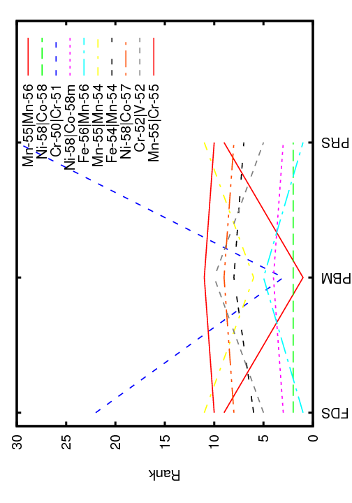
Figure 2: Comparison of the Alloy test case results, showing the first ten interactions according to the Pathways Based Metric $S_{PBM}$, ranked accordingly.

3.2.2 Alloy+c

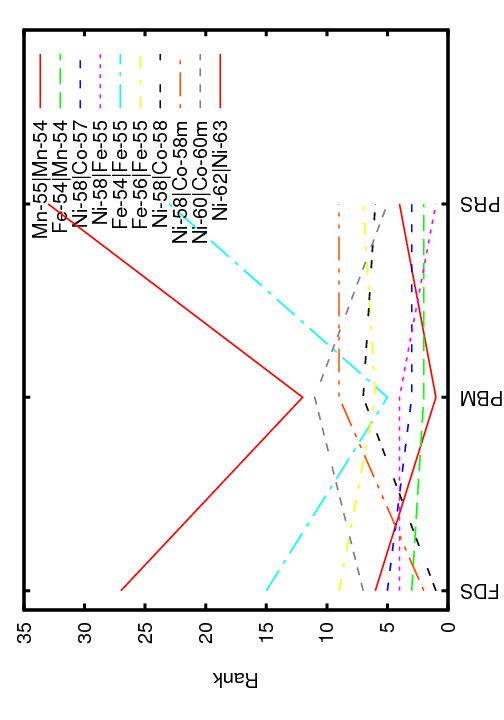
Figure 5: Comparison of the Alloy+c test case results, showing the first ten interactions according to the Pathways Based Metric $S_{PBM}$ for which comparison is possible.

See Table 4, Table 5, Table 6, Figure 3, Figure 4 and Figure 5.

Table 4 suggests that once the Pearson correlation becomes below $0.1$ it becomes inaccurate. Figure 3 shows that the smaller Pearson coefficients vary erratically with sampling, from which it is inferred that round-off effects have become important.

As indicated in Table 1 this case involves both an irradiation phase and a cooling period. Care is required in comparing the FDM approach in this instance, for the method uses only the matrix for the cooling phase, whereas the other analyses are of the entire history. Although there is still reasonably good correlation between $P_{FDS}$ and $P_{PRS}$, it is not as good in the other test cases.

Table 4: Alloy+c case. Values of absolute Pearson correlation coefficient $|r|$ as Monte Carlo sample size increases with $N_{x}$.

		Absolute Pearson
Parent	Child	$40$	$160$	$640$
Ni-58	Fe-55	$0.81342$	$0.79097$	$0.79709$
Fe-54	Mn-54	$0.48716$	$0.48798$	$0.48761$
Ni-58	Co-57	$0.24152$	$0.23469$	$0.23442$
Mn-55	Mn-54	$0.17194$	$0.16534$	$0.16563$
Ni-60	Co-60m	$0.16462$	$0.15008$	$0.13389$
Ni-58	Co-58	$0.13754$	$0.12544$	$0.11864$
Fe-56	Fe-55	$9.410\times 10^{-2}$	$7.202\times 10^{-2}$	$9.237\times 10^{-2}$
Ni-60	Co-60	$0.10390$	$6.218\times 10^{-2}$	$5.669\times 10^{-2}$
Ni-58	Co-58m	$6.996\times 10^{-2}$	$5.098\times 10^{-2}$	$4.101\times 10^{-2}$
Ti-46	Sc-46m	$3.614\times 10^{-2}$	$1.570\times 10^{-3}$	$1.575\times 10^{-2}$
Ti-47	Sc-46	$2.538\times 10^{-2}$	$2.806\times 10^{-3}$	$1.209\times 10^{-2}$
V-49	Sc-46	$4.678\times 10^{-3}$	$1.198\times 10^{-2}$	$1.144\times 10^{-2}$
Co-60m	Co-60	$1.923\times 10^{-2}$	$9.042\times 10^{-3}$	$8.303\times 10^{-3}$
Cr-50	V-50	$9.279\times 10^{-3}$	$1.598\times 10^{-2}$	$8.073\times 10^{-3}$
Ni-60	Co-59	$1.648\times 10^{-2}$	$1.167\times 10^{-2}$	$7.639\times 10^{-3}$
Ni-57	Co-57	$1.665\times 10^{-2}$	$1.499\times 10^{-2}$	$7.389\times 10^{-3}$
Co-57	Co-58	$2.483\times 10^{-3}$	$1.572\times 10^{-2}$	$6.780\times 10^{-3}$
Fe-54	Cr-51	$2.407\times 10^{-2}$	$2.252\times 10^{-2}$	$6.773\times 10^{-3}$
Co-57	Co-58m	$3.906\times 10^{-2}$	$9.176\times 10^{-3}$	$6.739\times 10^{-3}$
Ti-47	Ti-46	$2.828\times 10^{-2}$	$1.220\times 10^{-2}$	$5.516\times 10^{-3}$
Co-59	Fe-59	$8.709\times 10^{-3}$	$1.451\times 10^{-2}$	$5.499\times 10^{-3}$
Fe-58	Fe-59	$2.626\times 10^{-2}$	$1.466\times 10^{-2}$	$5.289\times 10^{-3}$
Fe-54	Fe-55	$2.698\times 10^{-2}$	$7.802\times 10^{-3}$	$5.261\times 10^{-3}$
Co-58	Fe-58	$2.502\times 10^{-3}$	$1.069\times 10^{-3}$	$5.199\times 10^{-3}$
Ti-47	Sc-46m	$4.156\times 10^{-3}$	$1.867\times 10^{-2}$	$5.039\times 10^{-3}$
Cr-50	Cr-51	$1.015\times 10^{-2}$	$2.073\times 10^{-3}$	$4.815\times 10^{-3}$
Co-59	Co-60	$1.789\times 10^{-2}$	$1.673\times 10^{-2}$	$4.743\times 10^{-3}$
Ni-58	Ni-59	$2.777\times 10^{-3}$	$1.273\times 10^{-2}$	$4.581\times 10^{-3}$
Mn-55	Mn-56	$1.473\times 10^{-2}$	$3.741\times 10^{-3}$	$4.456\times 10^{-3}$
Co-58	Co-59	$5.478\times 10^{-3}$	$6.033\times 10^{-4}$	$4.220\times 10^{-3}$

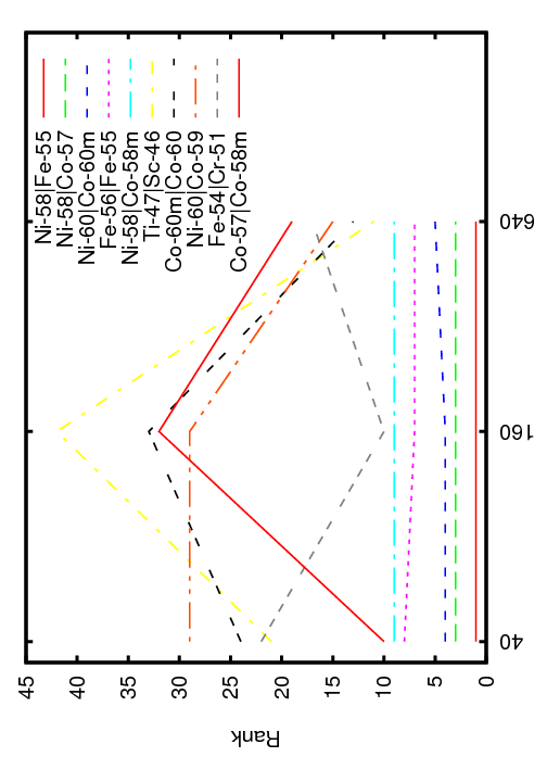
Figure 3: Comparison of the Alloy+c test case results, showing the first ten odd-numbered interactions according to the scaled Pearson technique value $S_{PRS}$, for a Monte-Carlo sample size of $N_{x}=640$ per reaction, as $N_{x}$ is increased.

Table 5: Alloy+c case. Rankings for different methods.

		Sensitivity
Parent	Child	FDS	PBM	PRS
Cr-52	Cr-51	$11$	$39$	$49$
Mn-55	Mn-54	$6$	$1$	$4$
Fe-56	Fe-55	$9$	$6$	$7$
Ni-58	Co-57	$5$	$3$	$3$
Ni-58	Ni-57	$16$	$20$	$42$
Ni-58	Co-58	$1$	$7$	$6$
Ni-58	Co-58m	$2$	$9$	$9$
Ni-58	Fe-55	$4$	$4$	$1$
Fe-54	Cr-51	$8$	$40$	$17$
Fe-54	Mn-54	$3$	$2$	$2$
Cr-50	Cr-51	$13$	$26$	$26$
Ni-62	Fe-59	$12$	$37$	$44$
Ni-60	Co-60	$10$	$14$	$8$
Ni-60	Co-60m	$7$	$11$	$5$
Fe-54	Fe-55	$15$	$5$	$23$
Cr-50	V-49	$14$	$16$	$35$
Fe-58	Fe-59	$18$	$27$	$22$
Fe-54	Mn-53	$17$	$18$	$30$
Ni-60	Co-59	$22$	$28$	$15$
Ni-59	Co-58	$21$	$0$	$0$
Ni-58	Fe-54	$31$	$0$	$0$
Ni-59	Co-58m	$23$	$0$	$0$
Co-59	Fe-59	$19$	$42$	$20$
Co-59	Co-58	$26$	$0$	$0$
Fe-56	Mn-55	$30$	$0$	$0$
Co-59	Co-58m	$25$	$0$	$0$
Ni-59	Fe-55	$32$	$0$	$0$
Ni-62	Ni-63	$27$	$12$	$33$
Fe-55	Mn-54	$28$	$0$	$0$
Co-58	Co-57	$24$	$30$	$34$
Co-57	Co-56	$29$	$44$	$37$
Co-58	Mn-54	$33$	$0$	$0$
Co-58	Co-58m	$20$	$62$	$0$

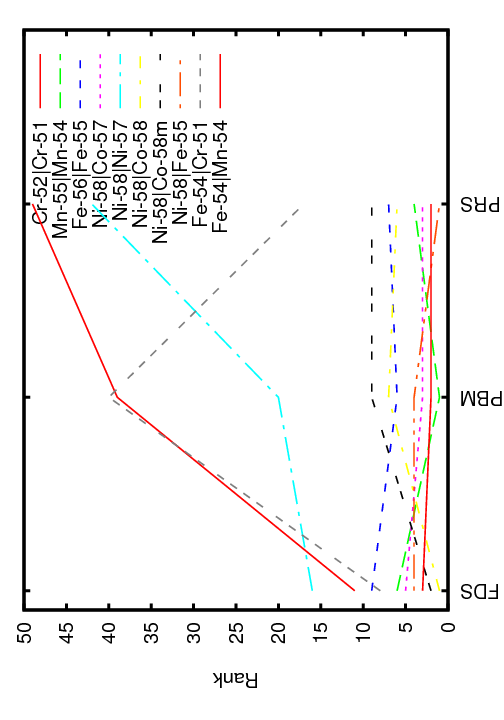
Figure 4: Comparison of the Alloy+c test case results, showing the first ten interactions by magnitude of Fréchet derivative. The labels are ordered according to Fréchet derivative size, so that the top interaction is the most sensitive.

Table 6: Alloy+c case. Rankings for different methods.

		Sensitivity
Parent	Child	FDS	PBM	PRS
Mn-55	Mn-54	$6$	$1$	$4$
Fe-54	Mn-54	$3$	$2$	$2$
Ni-58	Co-57	$5$	$3$	$3$
Ni-58	Fe-55	$4$	$4$	$1$
Fe-54	Fe-55	$15$	$5$	$23$
Fe-56	Fe-55	$9$	$6$	$7$
Ni-58	Co-58	$1$	$7$	$6$
Co-60m	Co-60	$0$	$8$	$13$
Ni-58	Co-58m	$2$	$9$	$9$
Co-58m	Co-58	$0$	$10$	$32$
Ni-60	Co-60m	$7$	$11$	$5$
Ni-62	Ni-63	$27$	$12$	$33$
Co-58	Co-59	$0$	$13$	$31$
Ni-60	Co-60	$10$	$14$	$8$
Co-59	Co-60m	$0$	$15$	$43$
Cr-50	V-49	$14$	$16$	$35$
Co-59	Co-60	$0$	$17$	$27$
Fe-54	Mn-53	$17$	$18$	$30$
Mn-53	Mn-54	$0$	$19$	$46$
Ni-57	Co-57	$0$	$21$	$16$
Ni-58	Ni-57	$16$	$20$	$42$
Mn-55	Mn-56	$0$	$23$	$29$
Mn-56	Fe-56	$0$	$22$	$0$
Co-58m	Co-59	$0$	$24$	$36$
Co-57	Co-58	$0$	$25$	$18$
Cr-50	Cr-51	$13$	$26$	$26$
Fe-58	Fe-59	$18$	$27$	$22$
Ni-60	Co-59	$22$	$28$	$15$
Ni-64	Ni-63	$0$	$29$	$39$
Co-58	Co-57	$24$	$30$	$34$

3.2.3 Fe

See Table 7 and Figure 6.

Table 7: Fe case. Rankings for different methods.

		Sensitivity
Parent	Child	FDS	PBM	PRS
Fe-56	Mn-56	$1$	$1$	$1$
Fe-56	Fe-55	$4$	$4$	$3$
Fe-54	Cr-51	$3$	$5$	$4$
Fe-54	Mn-54	$2$	$2$	$2$
Fe-57	Mn-56	$13$	$0$	$0$
Fe-57	Mn-57	$5$	$7$	$6$
Fe-54	Fe-55	$6$	$3$	$27$
Fe-56	Mn-55	$7$	$27$	$18$
Fe-58	Fe-59	$9$	$6$	$25$
Fe-58	Cr-55	$10$	$19$	$8$
Fe-58	Mn-58m	$11$	$21$	$19$
Fe-58	Mn-58	$12$	$22$	$22$
Fe-54	Mn-53	$8$	$9$	$7$
Fe-56	Fe-57	$16$	$10$	$11$
Fe-55	Mn-54	$14$	$0$	$0$
Cr-54	Cr-55	$20$	$15$	$12$
Cr-54	V-54	$21$	$26$	$5$
Mn-55	Cr-55	$18$	$24$	$26$
Mn-55	V-52	$22$	$25$	$16$
Mn-55	Mn-56	$15$	$0$	$0$
Fe-57	Fe-58	$25$	$13$	$24$
Mn-55	Mn-54	$24$	$0$	$0$
Fe-57	Cr-54	$27$	$28$	$14$
V-51	V-52	$32$	$16$	$23$
Mn-53	Mn-54	$19$	$8$	$10$
Fe-57	Fe-56	$23$	$0$	$0$
Co-59	Co-60m	$30$	$12$	$21$
Co-59	Mn-56	$31$	$0$	$0$
Co-59	Fe-59	$28$	$0$	$0$
Fe-55	Mn-55	$17$	$23$	$17$

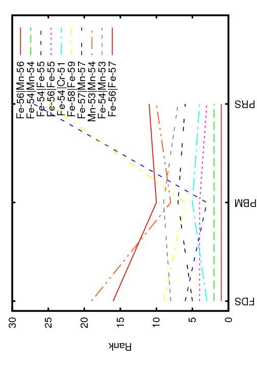
Figure 6: Comparison of the Fe test case results, showing the first ten interactions according to the Pathways Based Metric $S_{PBM}$, ranked accordingly.

3.2.4 LiMix

See Table 8 and Figure 7. The comparison between the various metrics in Figure 7 does not at first appear to be as successful as in other cases. However the dominant interaction from the PBM involves tritium for which uncertainty data are not accessible in the database, hence the FDS and PRS cannot assign it a ranking and it is omitted from the plot. Moreover all FDS rankings over $21$ similarly correspond to zero uncertainty and allowing for this, the comparison is as good as any reported herein.

Table 8: LiMix case. Rankings for different methods.

		Sensitivity
Parent	Child	FDS	PBM	PRS
Li-7	He-6	$3$	$5$	$3$
Li-7	Li-8	$2$	$3$	$2$
Be-9	He-6	$1$	$2$	$1$
O-16	N-16	$22$	$4$	$16$
Li-6	He-6	$4$	$7$	$5$
Li-7	Li-6	$24$	$0$	$0$
Be-9	Be-10	$6$	$10$	$7$
O-18	O-19	$8$	$11$	$10$
O-18	C-15	$5$	$8$	$13$
O-17	N-16	$15$	$0$	$0$
O-17	N-17	$7$	$12$	$12$
O-16	N-15	$18$	$14$	$11$
Be-9	Li-7	$11$	$0$	$0$
He-3	H-3	$25$	$0$	$0$
Be-10	He-6	$27$	$0$	$0$
Be-10	Be-11	$21$	$9$	$15$
O-16	O-17	$14$	$18$	$4$
Li-6	Li-7	$13$	$0$	$0$
N-15	N-16	$19$	$0$	$0$
N-15	C-15	$12$	$0$	$0$
N-15	B-12	$9$	$13$	$6$
C-13	Be-10	$10$	$16$	$8$
O-16	C-13	$23$	$15$	$17$
C-13	Be-9	$26$	$0$	$0$
O-17	O-18	$20$	$0$	$0$
O-17	N-15	$17$	$20$	$9$
O-17	O-16	$16$	$0$	$0$

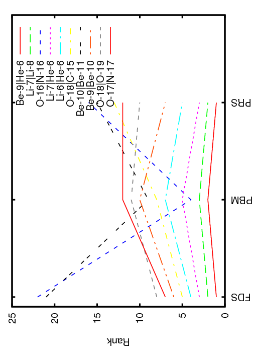
Figure 7: Comparison of the LiMix test case results, showing the first ten interactions according to the Pathways Based Metric $S_{PBM}$ for which comparison is possible.

3.2.5 WMix

See Table 9, , Table 10, Table 11, Figure 8, Figure 9 and Figure 10. Table 9 suggests that once the Pearson correlation becomes below $0.1$ it becomes inaccurate. Figure 8 shows that the lower rankings in terms of sensitivity vary erratically with sampling for similar reasons to do with round-off effects.

Table 9: WMix case. Values of absolute Pearson correlation coefficient $|r|$ as Monte Carlo sample size increases with $N_{x}$.

		Absolute Pearson
Parent	Child	$40$	$160$	$640$
Re187	Re188	$0.93702$	$0.94033$	$0.94091$
Ir193	Ir194	$0.24971$	$0.23407$	$0.24135$
Ir191	Ir192	$0.13306$	$0.13520$	$0.13542$
Ir193	Ir193m	$0.11155$	$0.11969$	$0.11550$
Re185	Re186	$0.10156$	$8.413\times 10^{-2}$	$7.955\times 10^{-2}$
W-184	W-185	$6.398\times 10^{-2}$	$9.215\times 10^{-2}$	$7.856\times 10^{-2}$
W-186	W-187	$5.029\times 10^{-2}$	$6.135\times 10^{-2}$	$6.423\times 10^{-2}$
Re187	Re188m	$2.181\times 10^{-2}$	$5.108\times 10^{-2}$	$5.264\times 10^{-2}$
Pt192	Pt191	$4.270\times 10^{-2}$	$4.238\times 10^{-2}$	$3.215\times 10^{-2}$
Ir193m	Ir193	$2.090\times 10^{-3}$	$9.212\times 10^{-3}$	$2.514\times 10^{-2}$
Ir191	Ir192m	$3.290\times 10^{-2}$	$1.785\times 10^{-2}$	$2.510\times 10^{-2}$
W-186	W-185m	$4.033\times 10^{-2}$	$4.676\times 10^{-2}$	$2.323\times 10^{-2}$
Re187	Re186	$3.941\times 10^{-2}$	$2.248\times 10^{-2}$	$1.720\times 10^{-2}$
Bi209	Bi210	$6.132\times 10^{-5}$	$1.141\times 10^{-2}$	$1.679\times 10^{-2}$
Ir192	Ir193m	$1.539\times 10^{-2}$	$1.425\times 10^{-2}$	$1.637\times 10^{-2}$
Ir192	Ir193	$1.845\times 10^{-2}$	$1.529\times 10^{-2}$	$1.352\times 10^{-2}$
W-182	W-181	$1.497\times 10^{-2}$	$1.685\times 10^{-2}$	$1.274\times 10^{-2}$
Ir191	Ir190	$2.775\times 10^{-2}$	$8.743\times 10^{-3}$	$1.263\times 10^{-2}$
Pb208	Pb207m	$3.345\times 10^{-2}$	$9.360\times 10^{-3}$	$1.217\times 10^{-2}$
Ir191	Ir191m	$2.715\times 10^{-2}$	$1.390\times 10^{-2}$	$1.167\times 10^{-2}$
Pt194	Pt193m	$1.482\times 10^{-2}$	$1.318\times 10^{-2}$	$1.020\times 10^{-2}$
W-186	W-185	$3.379\times 10^{-2}$	$1.427\times 10^{-2}$	$9.663\times 10^{-3}$
W-183	W-183m	$2.160\times 10^{-3}$	$1.927\times 10^{-2}$	$9.005\times 10^{-3}$
W-183	W-184	$5.385\times 10^{-3}$	$1.532\times 10^{-3}$	$8.812\times 10^{-3}$
Ir193	Ir192	$2.121\times 10^{-2}$	$8.499\times 10^{-3}$	$8.497\times 10^{-3}$
Re185	Re184m	$1.874\times 10^{-2}$	$7.629\times 10^{-3}$	$8.467\times 10^{-3}$
Ir194	Ir195m	$4.688\times 10^{-3}$	$5.884\times 10^{-3}$	$8.447\times 10^{-3}$
Ir193	Os193	$3.587\times 10^{-4}$	$2.355\times 10^{-3}$	$8.253\times 10^{-3}$
Re188m	Re188	$1.010\times 10^{-2}$	$4.477\times 10^{-3}$	$7.839\times 10^{-3}$
Bi210m	Bi210	$1.836\times 10^{-2}$	$3.068\times 10^{-3}$	$7.527\times 10^{-3}$

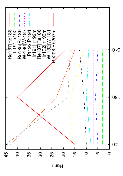
Figure 8: Comparison of the WMix test case results, showing the first ten odd-numbered interactions according to the scaled Pearson technique value $S_{PRS}$, for a Monte-Carlo sample size of $N_{x}=640$ per reaction, as $N_{x}$ is increased.

Table 10: WMix case. Rankings for different methods.

		Sensitivity
Parent	Child	FDS	PBM	PRS
Bi209	Bi210	$14$	$38$	$14$
Re187	W-185m	$29$	$0$	$0$
Re187	Re188m	$6$	$12$	$8$
Ir193	Os191	$35$	$0$	$0$
Ir193	Os191m	$37$	$0$	$0$
Bi209	Pb207m	$28$	$0$	$0$
Ir193	Ir192m	$11$	$0$	$0$
Re187	W-185	$31$	$0$	$0$
W-184	W-185m	$17$	$50$	$51$
Re187	W-187	$19$	$0$	$0$
Ir193	Ir193m	$3$	$16$	$4$
Re187	Ta183	$32$	$0$	$0$
W-186	W-185m	$7$	$27$	$12$
Re187	Re186	$8$	$18$	$13$
Re187	Re188	$1$	$4$	$1$
Pt194	Os191	$26$	$0$	$0$
Pt194	Os191m	$30$	$0$	$0$
Pb208	Pb207m	$12$	$26$	$19$
Re185	W-185m	$20$	$0$	$0$
Ir193	Ir192	$9$	$20$	$26$
W-184	W-185	$4$	$13$	$6$
Ir193	Ir194	$2$	$1$	$2$
Pt194	Ir193m	$34$	$0$	$0$
W-186	W-185	$10$	$21$	$22$
W-184	Ta183	$33$	$0$	$0$
W-184	Ta182m	$38$	$0$	$0$
W-184	Ta182	$36$	$0$	$0$
W-184	W-183m	$15$	$35$	$55$
Pt194	Ir194	$24$	$0$	$0$
Pt194	Pt193m	$13$	$24$	$21$

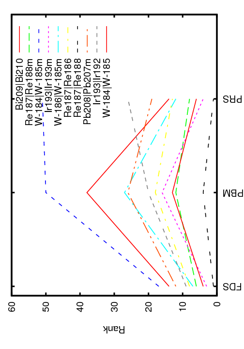
Figure 9: Comparison of the WMix test case results, showing the first ten interactions by magnitude of Fréchet derivative. The labels are ordered according to Fréchet derivative size, so that the top interaction is the most sensitive.

Table 11: WMix case. Rankings for different methods.

		Sensitivity
Parent	Child	FDS	PBM	PRS
Ir193	Ir194	$2$	$1$	$2$
Re185	Re186	$0$	$2$	$5$
Ir191	Ir192m	$0$	$3$	$11$
Re187	Re188	$1$	$4$	$1$
Ir191	Ir192	$0$	$5$	$3$
Ir192m	Ir192	$0$	$6$	$71$
Ir192	Ir193m	$0$	$7$	$15$
W-186	W-187	$5$	$8$	$7$
Ir193m	Ir193	$0$	$9$	$10$
Ir192	Ir193	$0$	$10$	$16$
W-187	Re187	$0$	$11$	$0$
Re187	Re188m	$6$	$12$	$8$
W-184	W-185	$4$	$13$	$6$
Re186	W-186	$0$	$14$	$37$
Re188m	Re188	$0$	$15$	$29$
Ir193	Ir193m	$3$	$16$	$4$
W-185	Re185	$0$	$17$	$0$
Re187	Re186	$8$	$18$	$13$
Ir194	Ir195	$0$	$19$	$62$
Ir193	Ir192	$9$	$20$	$26$
W-186	W-185	$10$	$21$	$22$
W-182	W-181	$0$	$22$	$17$
Pb207	Pb207m	$0$	$23$	$54$
Pt194	Pt193m	$13$	$24$	$21$
Ir194	Pt194	$0$	$25$	$0$
Pb208	Pb207m	$12$	$26$	$19$
W-186	W-185m	$7$	$27$	$12$
Ir191	Ir191m	$0$	$28$	$20$
Re186	Os186	$0$	$29$	$0$
Os186	Os185	$0$	$30$	$38$

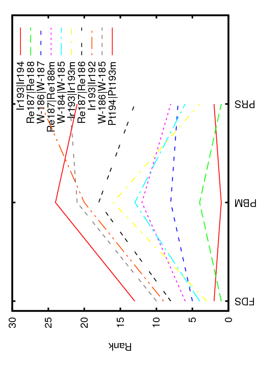
Figure 10: Comparison of the WMix test case results, showing the first ten interactions according to the Pathways Based Metric $S_{PBM}$ for which comparison is possible.

3.2.6 Y2O3

This very simple case illustrates the ranking process in additional detail, giving examples of the nuclear data that is used in the calculations. Following irradiation, the activity at the end of this test case is dominated ($99.6$ %) by two nuclides N-16 and Y-89m, see Table 12 for details. The pathways analysis performed routinely by Fispact-II shows that all pathways leading the $6$ nuclides listed, consist of just one reaction.

Table 12: Y2O3 case. First five radio-nuclides in final inventory, ordered by activity, plus Sr-89. Half-lives from the EASY-II database.

Order	Nuclide	Activity		Atoms	Half-life
		Bq	Percent		$\tau_{k}$
1	Y-89m	$2.5874\times 10^{7}$	$89.28\%$	$5.847\times 10^{8}$	$15.663s$
2	N-16	$2.9911\times 10^{6}$	$10.32\%$	$3.077\times 10^{7}$	$7.13s$
3	Rb-86m	$1.0193\times 10^{5}$	$0.35\%$	$8.971\times 10^{6}$	$1.017m$
4	C-15	$1.0083\times 10^{4}$	$0.04\%$	$3.562\times 10^{4}$	$2.449s$
5	Y-88	$1.191\times 10^{3}$	$0.004\%$	$1.583\times 10^{10}$	$107d$
9	Sr-89	$62$	$0.0002\%$	$3.891\times 10^{8}$	$50.57d$

Table 13: Y2O3 case. Reactions identified as important by pathways analysis. Note that apart from the reactions involving an excited parent species (labelled ‘m’) each reaction is equivalent to a pathway. For the notation describing each reaction see the Fispact-II manual.

Pathway	Cross-section	$\epsilon_{ij}$ Relative
Reaction	$barn$	Uncertainty %
O-16(n,p)N-16	$0.03357$	$0.0$
O-17(n,p)N-17	$0.01020$	$27.0$
O-18(n,a)C-15	$0.05645$	$28.0$
O-18(n,d)N-17	$8.9740\times 10^{-6}$	$23.0$
Rb-86m(b)Rb-86	$2.2675$	$4.39$
Y-89(n,a)Rb-86	$0.0036110$	$70.0$
Y-89(n,a)Rb-86m	$0.001820$	$70.0$
Y-89(n,p)Sr-89	$0.02179$	$19.0$
Y-89(n,2n)Y-88	$0.88630$	$5.7$
Y-89(n,n)Y-89m	$0.4347$	$8.5$
Y-89(n,g)Y-90	$0.0022040$	$9.2$
Y-89(n,g)Y-90m	$2.1410\times 10^{-4}$	$9.2$
Y-90m(n,g)Y-90	$2.4633$	$4.51$

PRS

As a result of the dominance by two reactions, all the detailed rankings by Pearson apart from the first two are suspect, see Table 14 and Figure 11 in support of this contention. Moreover, no (zero) uncertainty estimate is provided for the O-16$|$N-16 reaction, see Table 13, the source of the N-16 in the final inventory. Thus the Pearson ranking is maximal, and in the other sections O-16$|$N-16 would have to be omitted from the comparison plots. Other important reactions are identified by inspection of comparison tables and plots such as Table 15 and Figure 12 respectively. On this basis, the reaction producing Sr-89 is identified as potentially important, hence its inclusion in Table 12.

Table 14: Y2O3 case. Values of absolute Pearson correlation coefficient $|r|$ as Monte Carlo sample size increases with $N_{x}$.

		Absolute Pearson
Parent	Child	$160$	$640$	$2560$
Y-89	Y-89m	$0.99945$	$0.99945$	$0.99948$
Y-89	Rb-86m	$5.664\times 10^{-2}$	$4.483\times 10^{-2}$	$2.851\times 10^{-2}$
O-18	C-15	$1.768\times 10^{-3}$	$1.504\times 10^{-4}$	$8.698\times 10^{-3}$
Y-90m	Y-90	$1.041\times 10^{-2}$	$1.250\times 10^{-2}$	$7.383\times 10^{-3}$
Y-89	Rb-86	$1.326\times 10^{-3}$	$1.010\times 10^{-2}$	$3.955\times 10^{-3}$
O-18	N-17	$2.644\times 10^{-2}$	$8.750\times 10^{-3}$	$3.389\times 10^{-3}$
Y-89	Y-90	$3.402\times 10^{-3}$	$6.061\times 10^{-3}$	$2.537\times 10^{-3}$
Y-89	Y-90m	$1.537\times 10^{-2}$	$2.666\times 10^{-3}$	$2.261\times 10^{-3}$
Rb-86m	Rb-86	$6.646\times 10^{-3}$	$1.651\times 10^{-2}$	$2.238\times 10^{-3}$
O-17	N-17	$1.821\times 10^{-2}$	$2.273\times 10^{-2}$	$1.766\times 10^{-3}$
Y-89	Y-88	$2.699\times 10^{-2}$	$1.402\times 10^{-2}$	$1.426\times 10^{-3}$
Y-89	Sr-89	$1.358\times 10^{-2}$	$1.085\times 10^{-2}$	$4.010\times 10^{-4}$
O-16	N-16	$2.585\times 10^{-16}$	$5.905\times 10^{-16}$	$1.552\times 10^{-15}$

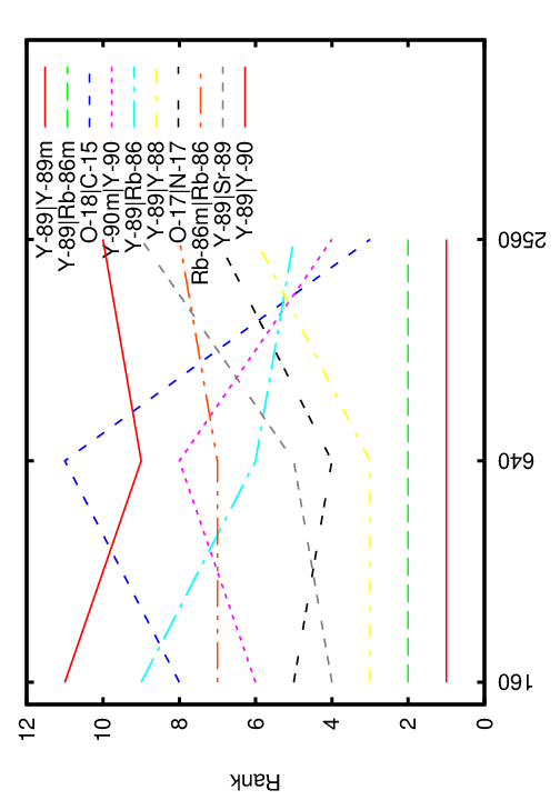
Figure 11: Comparison of the Y2O3 test case results, showing the first ten interactions according to the scaled Pearson technique value $S_{PRS}$, for a Monte-Carlo sample size of $N_{x}=2\,560$ per reaction, as $N_{x}$ is increased.

FDS

The Fréchet derivative method works with a matrix that has coefficients of all the possible reactions which involve the species by the standard Fispact-II pathways analysis. There seems to be little point in listing them all, obviously Table 13 is indicative. As in the case of Pearson, the absence of an uncertainty estimate for the O-16$|$N-16 reaction leads to a maximal ranking for the scaled Fréchet derivative, and in the other sections O-16$|$N-16 would have to be omitted from the comparison plots.

Table 15: Y2O3 case. Rankings for different methods.

		Sensitivity
Parent	Child	FDS	PBM	PRS
Y-89	Y-90m	$8$	$7$	$11$
Y-89	Rb-86m	$4$	$3$	$2$
O-16	N-16	$30$	$2$	$13$
Y-89	Rb-86	$5$	$10$	$5$
Y-89	Y-89m	$2$	$1$	$1$
Y-89	Y-90	$6$	$8$	$10$
Y-89	Sr-89	$3$	$9$	$9$
Y-89	Y-88	$1$	$5$	$6$
O-18	N-16	$11$	$0$	$0$
O-18	C-15	$7$	$4$	$3$
O-18	N-17	$12$	$11$	$12$
O-17	N-16	$9$	$0$	$0$
O-17	N-17	$10$	$6$	$7$
Y-88	Y-89m	$13$	$0$	$0$
O-16	O-17	$15$	$0$	$0$
Sr-89	Y-89m	$31$	$0$	$0$
Rb-86	Rb-86m	$14$	$0$	$0$
O-18	O-16	$21$	$0$	$0$
Y-90	Y-90m	$18$	$0$	$0$
Y-90	Rb-86m	$23$	$0$	$0$
O-18	O-17	$16$	$0$	$0$
O-17	O-18	$24$	$0$	$0$
Y-90	Rb-86	$22$	$0$	$0$
Y-90	Y-89m	$19$	$0$	$0$
Y-90	Sr-89	$20$	$0$	$0$
O-17	O-16	$17$	$0$	$0$
Y-89m	Y-90m	$28$	$0$	$0$
Y-89m	Rb-86m	$26$	$0$	$0$
Y-89m	Rb-86	$27$	$0$	$0$
Y-89m	Y-90	$29$	$0$	$0$
Y-89m	Sr-89	$25$	$0$	$0$

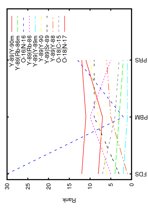
Figure 12: Comparison of the Y2O3 test case results, showing the first ten interactions by magnitude of Fréchet derivative. The labels are ordered according to Fréchet derivative size, so that the top interaction is the most sensitive.

PBM

Since all pathways leading to the most important nuclides in terms of activity, consist of just one reaction, it follows that these reactions are simply ranked in order of contribution of the child species to the final activity. Even though it has no associated uncertainty, the O-16$|$N-16 reaction can be ranked by PBM. Taking into account the fact that in the other sections O-16$|$N-16 would have to be omitted from the comparison plots, Figure 13 indicates that there is surprisingly good agreement between the methods, even for reactions that contribute little to the final activity.

Table 16: Y2O3 case. Rankings for different methods.

		Sensitivity
Parent	Child	FDS	PBM	PRS
Y-89	Y-89m	$2$	$1$	$1$
O-16	N-16	$30$	$2$	$13$
Y-89	Rb-86m	$4$	$3$	$2$
O-18	C-15	$7$	$4$	$3$
Y-89	Y-88	$1$	$5$	$6$
O-17	N-17	$10$	$6$	$7$
Y-89	Y-90m	$8$	$7$	$11$
Y-89	Y-90	$6$	$8$	$10$
Y-89	Sr-89	$3$	$9$	$9$
Y-89	Rb-86	$5$	$10$	$5$
O-18	N-17	$12$	$11$	$12$
Rb-86m	Rb-86	$0$	$12$	$8$
Y-90m	Y-90	$0$	$13$	$4$

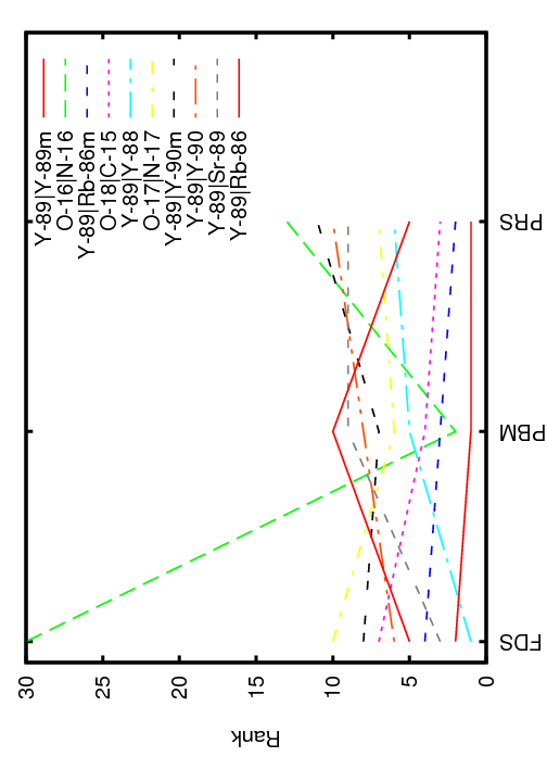
Figure 13: Comparison of the Y2O3 test case results, showing the first ten interactions according to the Pathways Based Metric $S_{PBM}$.

4 Conclusions

The sensitivity of the total activity of an inventory to uncertainties in the nuclear data for neutron-induced reactions has been studied. Six different test cases covering nearly the whole range of atomic masses were considered using three different ranking techniques. It is expected that similar results would be obtained for other inventory properties and other projectile particle species.

The principal result is that a simple pathways-based metric (PBM) gives a sensitivity ranking of interactions which is comparable to ranking based on more conventional measures obtained either by the direct method or in terms of Pearson correlation coefficients. Moreover, the PBM is superior in that it

1. is quick to calculate once the principal pathways have been identified

2. does not suffer from numerical difficulties such as underflow (Fréchet direct) or round-off (Pearson) in its evaluation

3. may be generalised to the case of multiple irradiation periods just like the pathways-reduced approach itself, whereas the other two techniques require further investigation.

4. does not require error estimates for every interaction coefficient like Pearson.

An additional noteworthy feature is that the PBM, which is a global measure of uncertainty, is comparable with more local measures, provided these others are scaled by the uncertainty in the reaction cross-section. This scaling is to be expected since the uncertainty estimates computed by Fispact-II [1, § A.13] involve a multiplication by a measure of cross-section uncertainty (r.m.s. is used to combine reaction coefficients rather than the simple percentages). However, the product also involves the number of child nuclides in the inventory which is a significantly different measure from the point sensitivity measures.

The value of studying a wide range of test cases is that it demonstrates the general applicability of the above conclusions. In conjunction with modifications to Fispact-II for more efficient pathways-based analysis in the presence of multiple irradiations, the PBM should be extended to account for loops in the pathways and ultimately integrated into a production version of the Fispact-II package.

Appendix: Fréchet Derivatives

As explained in Section 1, the Bateman equation Eq. (1)

$$\frac{dX}{dt}=\mathsf{A}X,\quad X(0)=X_{0},\quad t\in\left[0,t_{f}\right],$$

where $X\in\mathbb{R}^{n}$ is a vector of nuclide numbers and $\mathsf{A}\in\mathbb{R}^{n\times n}$ is a matrix of nuclear interaction coefficients, controls the evolution of the nuclear activation over time. In this appendix, we focus on the case where $\mathsf{A}$ is constant in time.

We are interested in the sensitivity of the total activity Eq. (2)

$$Q=\sum_{k=1}^{n}\lambda_{k}X_{k}(t_{f})$$

to the elements in $\mathsf{A}$, which is determined by the $n^{2}$ numbers $\partial Q/\partial A_{ij}$. To determine these quantities we use the matrix exponential and its Fréchet derivative. The matrix exponential of $\mathsf{A}\in\mathbb{R}^{n\times n}$ is defined by

$$e^{\mathsf{A}}=\sum_{k=1}^{\infty}\frac{\mathsf{A}^{k}}{k!}.$$

The Fréchet derivative of the exponential at $\mathsf{A}$ in the direction $\mathsf{E}\in\mathbb{R}^{{n\times n}}$ is denoted by $L_{\exp}(\mathsf{A},\mathsf{E})\in\mathbb{R}^{n\times n}$ and satisfies

$$e^{\mathsf{A}+\mathsf{E}}=e^{\mathsf{A}}+L_{\exp}(\mathsf{A},\mathsf{E})+o(\|\mathsf{E}\|)\,.$$

For further details of Fréchet derivatives see [15, Chap. 3].

The solution to the Bateman equation is given by

$$X(t)=e^{\mathsf{A}t}X_{0}$$

and so

$$Q=f^{T}X(t_{f})=f^{T}e^{\mathsf{A}t_{f}}X_{0},\qquad f=\left[\lambda_{1}\dots\ \lambda_{n}\right]^{T}.$$

Let $\mathsf{E}_{ij}$ be the ${n\times n}$ matrix with a $1$ in the $(i,j)$ entry and zeros elsewhere. Now,

$$\frac{\partial{Q}}{\partial A_{ij}} =\lim_{\delta\rightarrow 0}\frac{Q(A_{ij}+\delta)-Q(A_{ij})}{\delta}$$

$$=\lim_{\delta\rightarrow 0}\frac{f^{T}\left(e^{(\mathsf{A}+\mathsf{E}_{ij}\delta)t_{f}}-e^{\mathsf{A}t_{f}}\right)X_{0}}{\delta}$$

$$=\lim_{\delta\rightarrow 0}\frac{f^{T}\left(L_{\exp}(\mathsf{A}t_{f},\mathsf{E}_{ij}t_{f}\delta)+o(\delta)\right)X_{0}}{\delta}$$

$$=t_{f}f^{T}L_{\exp}(\mathsf{A}t_{f},\mathsf{E}_{ij})X_{0},$$

where we have used the fact that $L_{\exp}$ is linear in its second argument.

To determine the $k$ largest of these derivatives we can simply compute them all and sort them. For this we can use the relationship [15, eq. (3.16)]

$$\exp\left(\begin{bmatrix}t\mathsf{A}&\mathsf{E}_{ij}\\ 0&t\mathsf{A}\end{bmatrix}\right)=\begin{bmatrix}e^{t\mathsf{A}}&L_{\exp}(t\mathsf{A},\mathsf{E}_{ij})\\ 0&e^{t\mathsf{A}}\end{bmatrix},$$ (15)

which yields the formula

$$\exp\left(\begin{bmatrix}t\mathsf{A}&\mathsf{E}_{ij}\\ 0&t\mathsf{A}\end{bmatrix}\right)\begin{bmatrix}0\\ X_{0}\end{bmatrix}=\begin{bmatrix}L_{\exp}(t\mathsf{A},\mathsf{E}_{ij})X_{0}\\ e^{t\mathsf{A}}X_{0}\end{bmatrix}.$$ (16)

Hence one method to compute $L_{\exp}(\mathsf{A}t_{f},\mathsf{E}_{ij})X_{0}$ is to apply the method from [16] to compute the product on the left-hand side and then read off the first $n$ components.

However, it is not necessary to carry out $n^{2}$ Fréchet derivative evaluations. One suffices, as we now explain. We need some notation. The Kronecker product of two matrices is now text-book for numerical linear algebra, see e.g. ref [17]. It is defined for matrices $\mathsf{B}$ and $\mathsf{C}$ (of any dimension) as the block matrix $\mathsf{B}\otimes\mathsf{C}=(b_{ij}\mathsf{C})$. The $\mathop{\mathrm{vec}}$ operator stacks the columns of a matrix one of top of each other from first to last, producing a long vector. We need the property that $\mathop{\mathrm{vec}}(L_{\exp}(\mathsf{A},\mathsf{E}))=\mathsf{K}(\mathsf{A})\mathop{\mathrm{vec}}(\mathsf{E})$, for some $n^{2}\times n^{2}$ matrix $\mathsf{K}(\mathsf{A})$ that satisfies $\mathsf{K}(\mathsf{A})^{T}=\mathsf{K}(\mathsf{A}^{T})$. Using the fact that the $\mathop{\mathrm{vec}}$ of a scalar is itself and the formula

$$\mathop{\mathrm{vec}}(\mathsf{A}\mathsf{X}\mathsf{B})=(\mathsf{B}^{T}\otimes\mathsf{A})\mathop{\mathrm{vec}}(\mathsf{X})\,,$$

we have

$$\frac{\partial Q}{\partial A_{ij}} =t_{f}f^{T}L_{\exp}(\mathsf{A}t_{f},\mathsf{E}_{ij})X_{0}$$

$$=\mathop{\mathrm{vec}}\left(t_{f}f^{T}L_{\exp}(\mathsf{A}t_{f},\mathsf{E}_{ij})X_{0}\right)$$

$$=t_{f}(X_{0}\otimes f)^{T}\mathop{\mathrm{vec}}\left(L_{\exp}(\mathsf{A}t_{f},\mathsf{E}_{ij})\right)$$

$$\equiv t_{f}g^{T}\mathsf{K}(\mathsf{A}t_{f})\mathop{\mathrm{vec}}(\mathsf{E}_{ij}),$$

where $g=X_{0}\otimes f$. Now, since $\mathop{\mathrm{vec}}(\mathsf{E}_{ij})$ is a unit vector, we simply require the $k$ largest elements in modulus of $g^{T}\mathsf{K}(\mathsf{A}t_{f})$, which are the largest $k$ elements in magnitude of $\mathsf{K}(\mathsf{A}t_{f})^{T}g$. We have $\mathsf{K}(\mathsf{A}^{T}t_{f})g=\mathop{\mathrm{vec}}(L_{\exp}(\mathsf{A}^{T}t_{f},\mathsf{E}))$, where $\mathop{\mathrm{vec}}(\mathsf{E})=g=X_{0}\otimes f$ and hence $\mathsf{E}=fx_{0}^{T}$. This means that a single Fréchet derivative evaluation is sufficient, and it can be done using the relationship (15) above with an algorithm to compute the matrix exponential such as that in [18].

The computation of the exponential requires numerous matrix products, which can occasionally cause numerical over- or under-flow due to the large range of magnitudes in the coefficients arising in nuclear activation problems. This may necessitate the use of quadruple precision arithmetic on certain problems. In fact, quadruple precision was used to check the accuracy of all the Fréchet derivatives calculated in the course of the current work.

References

- [1] Sublet, J.-C. and Eastwood, J.W. and Morgan, J.G. The FISPACT-II User Manual. Issue 6. Technical Report CCFE-R(11)11, CCFE, June 2014.
- [2] Arter, W. and Morgan, J.G. Sensitivity analysis for activation problems. In Joint International Conference on Supercomputing in Nuclear Applications and Monte Carlo 2013, page 02404, 2014. http://dx.doi.org/10.1051/snamc/201402404.
- [3] Eastwood, J.W. and Morgan, J.G. Pathways and uncertainty prediction in Fispact-II. In Joint International Conference on Supercomputing in Nuclear Applications and Monte Carlo 2013, 2013. http://dx.doi.org/10.1051/snamc/201402404.
- [4] J.W. Eastwood, J.G. Morgan, and J.-C. Sublet. Inventory uncertainty quantification using TENDL covariance data in Fispact-II. Nuclear Data Sheets, 123:84–91, 2015.
- [5] J.C. Helton, J.D. Johnson, C.J. Sallaberry, and C.B. Storlie. Survey of sampling-based methods for uncertainty and sensitivity analysis. Reliability Engineering & System Safety, 91(10–11):1175–1209, 2006.
- [6] M. Ionescu-Bujor and D.G. Cacuci. A comparative review of sensitivity and uncertainty analysis of large-scale systems. I: Deterministic methods. Nuclear Science and Engineering, 147(3):189–203, 2004.
- [7] D.G. Cacuci and M. Ionescu-Bujor. A comparative review of sensitivity and uncertainty analysis of large-scale systems. II: Statistical methods. Nuclear Science and Engineering, 147(3):204–217, 2004.
- [8] B.M. Adams, M.S. Ebeida, M.S. Eldred, J.D. Jakeman, L.P. Swiler, J.A. Stephens, D.M. Vigil, T.M. Wildey, W.J. Bohnhoff, K.R. Dalbey, J.P. Eddy, , K.T. Hu, L.E. Bauman, and P.D. Hough. DAKOTA, A Multilevel Parallel Object-Oriented Framework for Design Optimization, Parameter Estimation, Uncertainty Quantification, and Sensitivity Analysis: Version 6.0 User’s Manual. Technical report, Sandia Technical Report SAND2014-4633, Sandia National Laboratories, Albuquerque, NM, 2014.
- [9] Radiation Safety Information Computational Center, Oak Ridge National Laboratory. SCALE: A Comprehensive Modeling and Simulation Suite for Nuclear Safety Analysis and Design. Technical Report ORNL/TM-2005/39, Version 6.1, CCC-785, Oak Ridge National Laboratory, June 2011.
- [10] E. Patelli, M. Broggi, M. de Angelis, and M. Beer. Opencossan: An efficient open tool for dealing with epistemic and aleatory uncertainties. In Vulnerability, Uncertainty, and Risk, pages 2564–2573. American Society of Civil Engineers, 2014. DOI 10.1061/9780784413609.258.
- [11] EASY-II European Activation System. http://www.ccfe.ac.uk/EASY.aspx.
- [12] ANSWERS Software Service. http://www.answerssoftwareservice.com.
- [13] A.M. Dunker. Efficient calculation of sensitivity coefficients for complex atmospheric models. Atmospheric Environment, 15(7):1155–1161, 1981.
- [14] The MathWorks. MATLAB. The MathWorks, Inc., Natick, Massachusetts, United States, Release 2012a.
- [15] Nicholas J. Higham. Functions of Matrices: Theory and Computation. Society for Industrial and Applied Mathematics, Philadelphia, PA, USA, 2008.
- [16] Awad H. Al-Mohy and Nicholas J. Higham. Computing the action of the matrix exponential, with an application to exponential integrators. SIAM J. Sci. Comput., 33(2):488–511, 2011.
- [17] G.H. Golub and C.F. Van Loan. Matrix computations. 4th Edition. Johns Hopkins, Baltimore, 2013.
- [18] Awad H. Al-Mohy and Nicholas J. Higham. A new scaling and squaring algorithm for the matrix exponential. SIAM J. Matrix Anal. Appl., 31(3):970–989, August 2009.